Surrogate Modeling for Building Design: Energy and Cost Prediction Compared to Simulation-Based Methods

Abstract

Designing energy-efficient buildings is essential for reducing global energy consumption and carbon emissions. However, traditional physics-based simulation models require substantial computational resources, detailed input data, and domain expertise. To address these limitations, this study investigates the use of three machine learning-based surrogate models—Random Forest (RF), Extreme Gradient Boosting (XGBoost), and Multilayer Perceptron (MLP)—trained on a synthetic dataset of 2000 EnergyPlus-simulated building design scenarios to predict both energy use intensity (EUI) and cost estimates for midrise apartment buildings in the Toronto area. All three models exhibit strong predictive performance, with R² values exceeding 0.9 for both EUI and cost. XGBoost achieves the best performance in cost prediction on the testing dataset with a root mean squared error (RMSE) of 5.13 CAD/m², while MLP outperforms others in EUI prediction with a testing RMSE of 0.002 GJ/m². In terms of computational efficiency, the surrogate models significantly outperform a physics-based simulation model, with MLP running approximately 340 times faster and XGBoost and RF achieving over 200 times speedup. This study also examines the effect of training dataset size on model performance, identifying a point of diminishing returns where further increases in data size yield minimal accuracy gains but substantially higher training times. To enhance model interpretability, SHapley Additive exPlanations (SHAP) analysis is used to quantify feature importance, revealing how different model types prioritize design parameters. A parametric design configuration analysis further evaluates the models’ sensitivity to changes in building envelope features. Overall, the findings demonstrate that machine learning-based surrogate models can serve as fast, accurate, and interpretable alternatives to traditional simulation methods, supporting efficient decision-making during early-stage building design.

1. Introduction

Buildings are among the largest contributors to global energy consumption and greenhouse gas (GHG) emissions, underscoring the urgent need for tools that facilitate faster and more efficient evaluation during early design stages [1]. Rapid and reliable assessments of both energy performance and cost at these stages can enable more informed decision-making by balancing environmental sustainability with economic feasibility.

A widely adopted method for assessing energy performance in early-stage building design is the use of physics-based simulation models. These tools, such as EnergyPlus, TRNSYS, and DesignBuilder, simulate building performance under varying design scenarios. For example, EnergyPlus has been used to quantify the benefits of envelope retrofits in historical buildings [2] and to evaluate the use of phase change materials (PCMs) in walls, resulting in a 6% reduction in annual energy consumption [3]. Similarly, TRNSYS and DesignBuilder have been employed in retrofit assessments, consistently demonstrating reductions in energy demand [4,5,6]. Physics-based simulation tools have also been widely applied in early-stage building design. For instance, Liu and Li [7] proposed a two-stage framework that integrates Building Information Modeling (BIM) with EnergyPlus to predict building energy consumption during the conceptual design phase. This framework enables rapid feedback and supports the exploration of passive design strategies early in the design process. Rasheed et al. [8] utilized TRNSYS to develop a Building Energy Simulation (BES) model for multi-span greenhouses. Their study examined the influence of design parameters on the internal thermal environment, demonstrating the utility of TRNSYS for performance-based assessments in the early stages of specialized building designs. Similarly, Benachir et al. [9] employed TRNSYS to simulate mechanical solar ventilation with phase change materials in building envelopes, highlighting the effectiveness of this tools in evaluating innovative design strategies during the early phases of building development.

Despite their value, these physics-based simulations are often time- and resource-intensive. They require detailed input data, expert knowledge, and substantial computational resources. Each design or retrofit scenario necessitates a separate simulation run, which may take several hours to days depending on model complexity [10]. These limitations hinder their practical use during the iterative, exploratory nature of early-stage design.

To address these challenges, data-driven approaches, particularly machine learning (ML)-based surrogate models, have gained attention as efficient alternatives. Trained on data generated from physics-based simulations, these models can approximate simulation outputs with high accuracy at a fraction of the computational cost. Surrogate models have been applied to various tasks, including conceptual design evaluations, sensitivity analyses, and design optimization [11].

Several studies have demonstrated the effectiveness of ML-based surrogate modeling in the building domain. For instance, Singaravel et al. [12] trained artificial neural networks (ANNs) and long short-term memory (LSTM) models on 800 simulation samples generated by EnergyPlus. Similarly, Rackes et al. [13] used support vector machines (SVMs) to predict energy performance, achieving an R² of approximately 0.97.

Recent systematic reviews highlight the rise of ML-based surrogate approaches as viable alternatives to physics-based simulation due to their speed and scalability. Ardabili et al. [14] and others categorize surrogate methods—such as ANNs, ensemble models, and GANs—for energy consumption forecasting, emphasizing the superior robustness of hybrid and deep learning models. Jiang et al. [15] further discuss physics-informed ML, which integrates physical principles to improve generalization in building performance tasks.

Despite the growing interest in surrogate modeling for building performance prediction, most existing studies primarily focus on energy consumption or thermal comfort as output variables, with limited integration of economic metrics. For example, Li et al. [16] introduced a data-driven modeling and optimization method for building energy performance in the design stage, focusing on energy metrics without incorporating cost considerations. Similarly, Hussien et al. [17] recently investigated the utilization of machine learning algorithms to predict long-term energy consumption in buildings, yet cost estimation was not included as part of the modeling scope. Another study [18] proposed a coupled modeling approach that leverages the capabilities of ML-based building performance simulation surrogate models and multi-objective optimization, enhancing model flexibility and reducing the number of additional simulations needed; however, it did not incorporate cost evaluation or address financial outcomes directly. These approaches, while demonstrating high predictive accuracy and adaptability, often assume an implicit separation between energy and cost evaluations, requiring separate tools or post-processing to estimate early-stage design costs or financial feasibility.

While joint consideration of performance and cost objectives has been widely explored in domains such as manufacturing and energy systems—often through formal multi-objective optimization—building design introduces additional complexity due to spatial variability, climate responsiveness, and regulatory diversity. Rather than employing a dual-objective optimization model, this study develops separate surrogate models to predict energy and cost outcomes based on the same underlying design inputs. This parallel prediction approach supports early-stage decision-making by enabling rapid, integrated evaluation without the computational burden of simulation or the structural assumptions required in traditional multi-objective frameworks.

In terms of dataset generation, dataset design and size have garnered limited attention. For instance, Heo et al. [19] used simulation data from EnergyPlus to train statistical models for retrofit evaluation but did not explore how varying the number of samples affected model generalizability or runtime. In 2024, a study [20] systematically assessed surrogate performance versus sample size, finding that random forest models exceed linear baselines above ~1000 samples, achieving MAE ~ 1.7 kWh/m². Furthermore, while some recent studies have applied explainable ML methods (e.g., SHAP or permutation importance), these are rarely combined with parametric sensitivity analyses to understand the robustness of design decisions for building early-stage designs. This disconnect limits the practical application of surrogate models in real-world design workflows where both predictive accuracy and interpretability are essential.

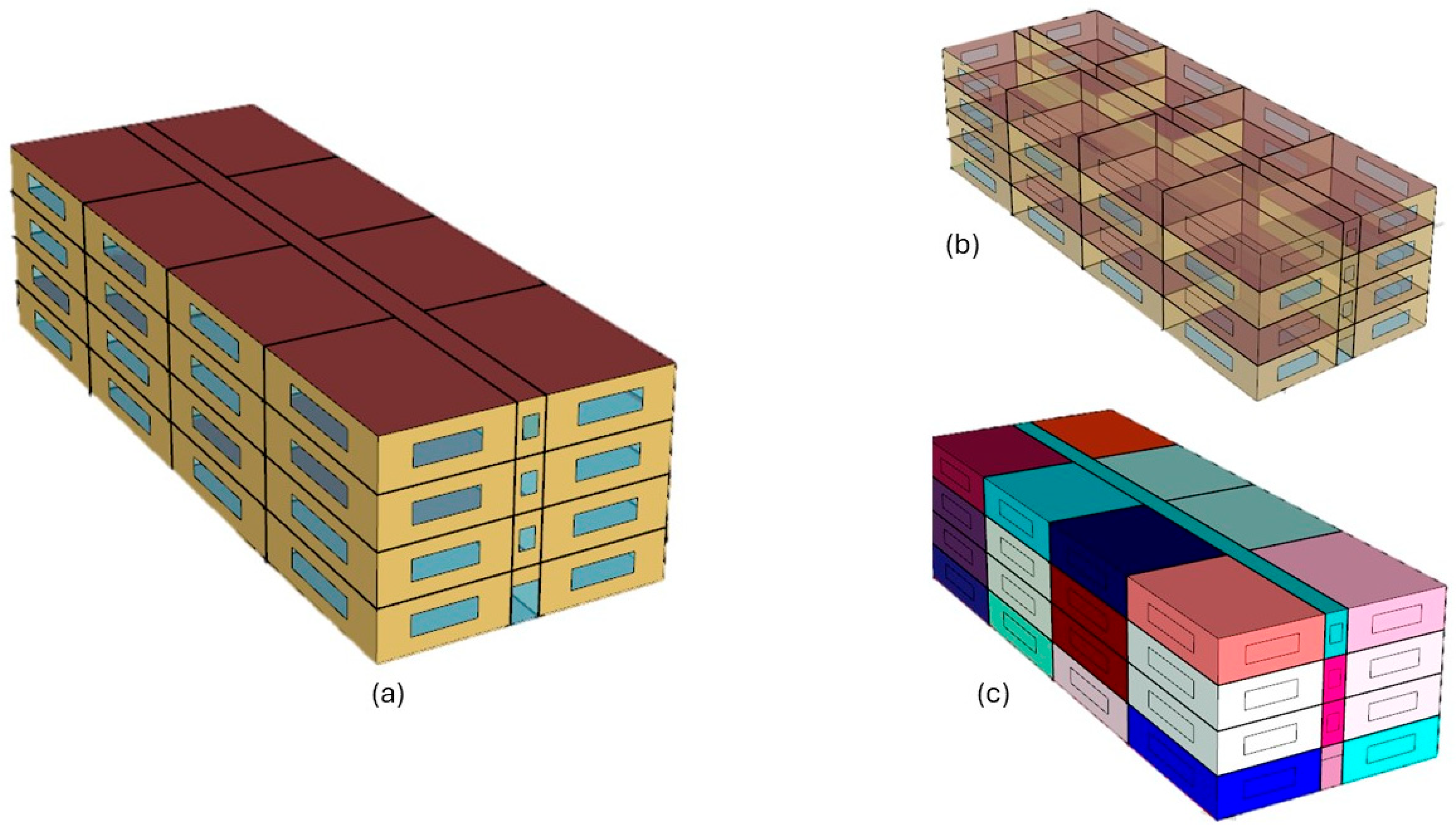
This study addresses key limitations in the use of simulation-based approaches for early-stage building design by developing machine learning-based surrogate models trained on EnergyPlus simulation outputs. In addition to predicting energy use intensity (EUI), this study introduces a cost estimation framework that quantifies costs across six key building components—envelope, heating and cooling, lighting, hot water, ventilation, and total equipment cost for each design scenario. Unlike previous studies, this work integrates detailed cost data into the synthetic dataset and trains separate machine learning models for predicting both energy performance and different design configuration costs. Although the surrogate modeling tool developed in this study is designed to accommodate multiple building types and climate zones across Canada, this paper focuses on midrise residential buildings located in Toronto. This building typology was selected due to its prevalence in Canadian urban centers and its relevance to current retrofit initiatives. Toronto was chosen as a representative urban climate zone to illustrate the capabilities of the proposed framework while maintaining methodological clarity.

A major contribution of this study is the demonstration that surrogate models can support rapid, integrated evaluation of energy and cost outcomes, thereby streamlining the decision-making process in early design stages. The influence of training dataset size on model performance is systematically investigated, and an optimal sample size is identified to balance predictive accuracy and computational efficiency. The application of SHAP-based interpretability methods reveals how different model architectures prioritize design features, offering transparent insights into model behavior. Finally, a parametric configuration analysis highlights model sensitivity to key envelope parameters, demonstrating the surrogate models’ potential—and limitations—for generalization. These findings collectively position the proposed framework as a practical tool for performance-driven building design.

The remainder of this paper is structured as follows: Section 2 details the methodology, including an overview of the process, synthetic data generation, preprocessing, ML models, and evaluation metrics. Section 3 analyzes the generated simulation data and selected building features. Section 4 presents the results and discussion, followed by the conclusion in Section 5.

2. Methodology

2.1. Overview

The overall workflow of this study is illustrated in Figure 1. The process begins with synthetic data generation using the Building Technology Assessment Platform (BTAP, an open-source toolkit for building performance simulation) [10], developed by Natural Resources Canada (NRCan) and powered by OpenStudio simulation engine (version 3.7.0). The Latin Hypercube Sampling (LHS) workflow within BTAP is utilized to randomly sample building design parameters across predefined ranges, creating diverse combinations of key building features.

For each sampled design, BTAP simulates hourly electricity and natural gas consumption alongside detailed cost estimations for major building components. This simulation is site-specific, incorporating relevant weather data for the Toronto area to ensure accurate energy performance and cost modeling. The synthetic dataset is then formatted into input features (predictors) and output variables (targets) and processed through a comprehensive preprocessing pipeline, including encoding of categorical variables and normalization of numerical features. Next, machine learning surrogate models, including Random Forest (RF), Extreme Gradient Boosting (XGBoost), and Multilayer Perceptron (MLP), are trained and evaluated using this preprocessed data to predict both energy use intensity (EUI) and building cost. Once trained and validated, these models can be saved and subsequently loaded to predict outcomes for new design scenarios, following standard machine learning deployment practices.

To interpret the model results and understand feature impacts, SHAP (SHapley Additive exPlanations) analysis is performed. This provides insight into the importance and contribution of each input feature to model predictions. Finally, design sensitivity analysis is conducted through parametric variation of key features. By systematically varying individual design parameters and observing their influence on predicted energy use and cost, the sensitivity and robustness of the surrogate models are assessed.

2.2. Synthetic Energy Simulation Data

The simulation data is produced using the BTAP [21], a tool developed by NRCan. BTAP enables the rapid generation of archetype buildings based on Canadian building codes and also various energy conservation measures and integrates them into Building Energy Models (BEMs) through computational scripts [22]. These models are created using OpenStudio [23] and simulated with EnergyPlus.

Latin Hypercube Sampling (LHS) is used to generate the simulation input data based on the combination of different building features. LHS is a powerful technique for generating diverse building simulation input datasets by systematically exploring different combinations of building features. By dividing each feature dimension into non-overlapping intervals with equal probability, LHS ensures a well-distributed and representative set of input scenarios [24]. This method reduces variability and improves the efficiency of simulations by capturing a wide range of possible building configurations while minimizing redundant sampling. Compared to memoryless methods like Monte Carlo (MC) sampling, LHS provides better coverage of the input space, reducing variance and requiring fewer samples to achieve reliable results.

In this study, a sample of 2000 buildings was selected for model training. Each building includes two distinct prediction targets: energy use intensity (EUI) and cost. The choice of 2000 buildings was based on prior experience, balancing computational efficiency with prediction accuracy. However, this sample size served only as a starting point. To evaluate whether this threshold was sufficient, a sensitivity analysis will be conducted in Section 4.5 (“Impact of Training Size”), where model performance was assessed using different training sample sizes for both energy and cost prediction tasks.

2.3. Costing Data

BTAP includes a module called BTAP-Costing [21], which estimates the capital cost of a building based on the same input features used for energy estimation. This module is developed and maintained by NRCan. The cost estimation relies on a costing database that includes material, labor, and equipment costs, primarily sourced from a third-party commercial costing agency, with some additional internal estimates for items not covered by the agency’s database [25]. The BTAP-Costing module provides cost estimates for various building components, such as heating and cooling equipment, the building envelope, and lighting. It also includes cost data for 70 different locations across Canada. It is important to note that individual design parameters do not carry explicit cost values as model inputs. Instead, the BTAP-Costing module estimates the total capital cost of a building configuration using internal rules and cost libraries based on the full set of input features.

2.4. Preprocessing

Before a dataset can be used to train a machine learning model or used for prediction, it needs to be preprocessed. This includes converting any categorical variables into numerical variables, removing unnecessary columns in the dataset, as well as separating the dataset into 3 smaller datasets: the training dataset, the validation dataset, and the testing dataset. The training dataset is used to train the machine learning models. This is where the machine learning models learn complex patterns to try to accurately predict the EUI and the costing. The validation dataset is then used to tune the hyperparameters of the models. Finally, when the machine learning models are tuned, the testing dataset is used to evaluate the performance of the final models. In this paper, 80% of the dataset is used for training, and the other 20% is used for testing. When training the machine learning models, 10% of the training dataset is used as the validation dataset.

After preprocessing the dataset, a feature selection process was implemented to improve model efficiency and reduce overfitting. A multi-task Lasso (MTL) regression model was employed, which is well-suited for problems involving multiple related target variables, such as predicting both energy and cost outcomes. This approach applies L1 regularization, encouraging sparsity by shrinking less important feature coefficients to zero [26]. The rationale for using MTL lies in the fact that energy use and cost are partially influenced by overlapping design parameters (e.g., insulation levels, HVAC type, and window-to-wall ratio). By enforcing shared sparsity across outputs, MTL identifies features that contribute meaningfully to both prediction tasks, supporting dimensionality reduction while maintaining performance. This method has been shown in recent literature to enhance generalization and model interpretability in multi-output regression problems where the targets are not fully independent. The model was fitted to the training data, and features were ranked based on the average absolute value of their regression coefficients across all tasks. Features with coefficients consistently equal to zero were excluded, as they contributed minimally to prediction performance. This filtering resulted in a final set of 16 features, detailed in

Table 1. Selected building features.

Feature Name	Definition	Range/Categories
dcv_type	Demand Control Ventilation (DCV) Strategy	Occupancy-based DCV CO2-based DCV No DCV
ecm_system_name	Dominant HVAC System Type	CCASHP/Electric Baseboard (Backup) CCASHP/VRF (Backup) ASHP/PTHP ASHP/Electric Baseboard (Backup) CGSHP and Chiller Plant (Fan Coil) ASHP/VRF (Backup)
erv_package	Energy Recovery Ventilator (ERV)	Plate-Existing (to required air loops) Plate-All (to all air loops) Rotary-Existing (to required air loops) Rotary-All (to all air loops)
nv_type	Natural Ventilation (NV)	NECB Default Add NV
airloop_economizer_type	Air Loop Economizer Type	NECB Default Differential Enthalpy Differential Dry Bulb
primary_heating_fuel	Main Heating Fuel	Electricity Natural Gas
boiler_eff	Boiler Efficiency	NECB Default 88% Efficient Condensing Boiler 96.2% Efficient Condensing Gas Boiler
furnace_eff	Furnace Efficiency	NECB Default 85% Efficient Furnace
shw_eff	Service Water Heater (SHW) Efficiency	NECB Default 91% efficient condensing gas SHW 94% efficient condensing gas SHW
ext_wall_cond	External Walls Thermal Conductance W/(m2∙K)	0.314 (R18) 0.278 (R20) 0.247 (R22) 0.21 (R27) 0.183 (R31)
ext_roof_cond	External Roofs Thermal Conductance W/(m2∙K)	0.227 0.193 0.183 0.162 0.142 0.138 0.121
fixed_window_cond	Fixed windows thermal conductance W/(m2∙K)	2.4 2.2 1.6
fixed_wind_solar_trans	The Solar Heat Gain Coefficient (SHGC) of fixed windows	Range 0.2–0.6 (Step = 0.1)
fdwr_set	Fenestration and Door-to-Walls Ratio	Range 0.1–0.7 (Step = 0.1)
srr_set	Skylight to Roof Ratio	0.03 0.05 0.08 0.10
rotation_degrees	Building’s Rotation	Range 0–359°

, which represent the most influential variables across energy and cost prediction tasks.

Additionally, before the preprocessed dataset is used for training, it needs to be scaled to improve the performance of the ML models. In this research, a standard scaler is used to standardize the values of each column in the dataset such that its distribution will have a mean of 0 and a standard deviation of 1. The transformed value ($z)$ could be calculated via the formula below:

$$z={\displaystyle \frac{\left(x-\mu \right)}{\sigma }}$$

(1)

where $\mu$ and $\sigma$ are the mean and standard deviation of the columns, respectively, and $x$ represents the original values in the column.

2.5. Machine Learning Models

Three machine learning algorithms—MLP, XGBoost, and RF—were selected to develop a surrogate model for building energy and cost prediction. These models were chosen for their ability to capture complex relationships within high-dimensional data. Two models were created for each machine learning algorithm. One for predicting EUI and the other for predicting cost values.

2.5.1. Multi-Layer Perceptron (MLP)

MLP is a type of artificial neural network consisting of multiple layers of neurons. The input layer receives the building features, while the hidden layers, equipped with a Rectified Linear Unit (ReLU) activation function, capture the nonlinear interactions between the features. The output layer predicts either the EUI or cost values.

While MLP is well-suited for data with nonlinear dependencies, it requires careful tuning of hyperparameters. Therefore, hyperparameter optimization was performed to find the optimal values for the number of hidden layers, the number of neurons in each hidden layer, the learning rate, the dropout rate, and the optimizer type. In this study, Hyperband optimization is used for hyperparameter tuning. This method systematically explored the parameter space (defined by the ranges listed in

Table 2. Tuned hyperparameter values for predicting energy and costing.

Model	Hyperparameter	EUI	Costing	Range
XGBoost	N estimators	500	500	[100, 250, 500]
	Max depth	10	5	[5, 10, 15]
	Learning rate	0.05	0.05	[0.01, 0.05, 0.1]
	Subsample	0.5	0.5	[0.5, 0.7, 1]
MLP	No. of hidden layers	2	2	(1, 3)
	No. of nodes in hidden layers [Layer1, Layer2, Layer3]	[856, 3744]	[2744, 248]	(8, 4096), step = 8
	Learning rate	0.001	0.001	[0.001, 0.0005, 0.0001, 0.00005, 0.00001]
	Dropout rate	0.0	0.0	[0.0, 0.05, 0.1, 0.2, 0.3]
	Optimizer	Adam	Adam	[Adam, SGD, RMSProp]
Random Forest	N estimators	100	100	[50, 100, 150]
	Max depth	None	15	[None, 5, 10, 15, 30]
	Min samples split	2	2	[2, 4, 8]
	Min samples leaf	1	1	[1, 2, 4]

, which were populated with commonly used values) by training and validating various combinations of hyperparameter values and keeping track of the configuration that achieved the lowest validation loss. Hyperband was chosen due to its suitability for models like MLP that involve expensive training processes. Its early-stopping mechanism enables efficient exploration of a large hyperparameter space while saving computational resources.

2.5.2. Random Forest (RF)

RF is an ensemble learning method that utilizes multiple decision trees and combines their outputs to improve prediction accuracy. One of its key strengths is the ability to handle high-dimensional data and effectively ignore irrelevant features. These characteristics make RF an ideal candidate for this research, which involves using a large number of building features as input data. Although RF generally requires less hyperparameter tuning compared to MLP, hyperparameter tuning was still conducted using randomized search to optimize the algorithm’s performance. This approach ran 70 iterations, with each configuration evaluated using 3-fold cross-validation. Randomized search was selected for RF, as it offers a computationally efficient method to explore a wide range of hyperparameters, which is adequate given RF’s lower sensitivity to parameter changes.

2.5.3. Extreme Gradient Boosting (XGBoost)

XGBoost, an advanced version of gradient boosting, also uses an ensemble of decision trees like the RF method. However, unlike RF, where trees are trained independently, XGBoost builds decision trees sequentially. Each new tree corrects the errors made by the previous ones, focusing on reducing prediction errors step by step. Parallelized computation makes XGBoost an efficient model for handling structured tabular building data.

Similar to MLP, XGBoost is sensitive to hyperparameters, requiring careful tuning for optimal performance. Therefore, key hyperparameters, such as the number of estimators, maximum depth, learning rate, and subsample ratio, were optimized to enhance the model’s prediction accuracy. Grid search with 3-fold cross-validation was employed to identify the optimal hyperparameters. Grid Search was used for XGBoost because the number of critical parameters was relatively small and exhaustive search was computationally feasible, allowing for a thorough evaluation of each configuration.

2.6. Evaluation

The performance of the machine learning models was evaluated using root mean squared error (RMSE), coefficient of determination ($R^2$), and mean absolute error (MAE). The primary metric chosen to evaluate the performance of the models in the training process is RMSE because it penalizes larger errors strongly compared to MAE and provides an error rate that is the same unit as the target variable [27]. The corresponding formula for its calculation is as follows:

$$RMSE=\sqrt{{\displaystyle \frac{{\sum }_{i=1}^N{\left(y_i-{\widehat{y}}_i\right)}^2}{N}}}$$

(2)

where ${\widehat{y}}_i$ and $y_i$ are the predicted and actual values, and $N$ is the total number of data points in the dataset.

Additional metrics such as MAE and $R^2$ were used to evaluate the performance of the machine learning models in the testing stage. Since MAE treats all errors equally, it is less sensitive to outliers compared to RMSE. This property gives us an additional metric to evaluate the models and is calculated using the formula below (3):

$$MAE={\displaystyle \frac{1}{N}}\sum _{i=1}^N\left|y_i-{\widehat{y}}_i\right|$$

(3)

Finally, $R^2$ provides a measure of how well the model’s predictions match the actual data. A high $R^2$ value indicates that the machine learning model is a good fit, whereas a low $R^2$ value indicates that the machine learning model is less accurate in predicting EUI and costing. Mathematically, $R^2$ is expressed as

$$R^2=1-{\displaystyle \frac{\sum _{i=1}^N{\left({\widehat{y}}_i-y_i\right)}^2}{\sum _{i=1}^N{\left(y_i-\overline{y}\right)}^2}}$$

(4)

where $\overline{y}$ is the average of the actual values.

2.7. SHAP Analysis

SHAP (SHapley Additive exPlanations) analysis was employed to interpret the predictions of the machine learning models and to quantify the contribution of each input feature. SHAP assigns an importance value to each feature based on Shapley values from cooperative game theory, providing a consistent framework for model interpretability. Larger absolute SHAP values indicate features with greater influence on the model’s output, while smaller values suggest less impact.

The SHAP framework developed by Lundberg and Lee [28] was used, which supports different model types through specific explainers. For the XGBoost model, the TreeExplainer, optimized for tree-based models, was applied. For MLP that is not tree-based, the model-agnostic KernelExplainer was used. To manage computational complexity while preserving feature diversity, the input dataset was sampled before computing SHAP values. For models with multiple prediction targets, SHAP values were averaged across outputs to provide an overall feature importance measure.

3. Simulation Data

Building Information

In this study, the selected building for simulation is a midrise apartment complex, primarily designated for commercial use, with a total of four stories and about 3135 m² of conditioned floor area and a ceiling-to-floor height of 3.05 m for each story. The building consists of 27 distinct thermal zones, which are illustrated in Figure 2c. The location of the building is in Toronto. Several building parameters, such as the heating and cooling system types, thermal conductance of the surfaces, and building rotation degree, were selected as predictors for training the machine learning model.

These parameters, which serve as inputs for the simulation, were chosen through a feature selection process to identify the most relevant factors for predicting EUI and cost estimates. A detailed list of these selected parameters can be found in Table 1.

In Table 1, in the ‘Dominant HVAC System Type’ row, VRF stands for Variable Refrigerant Flow, and ASHP, PTHP, CCASHP, and CGHSP stand for Air-Source Heat Pump, Packaged Terminal Heat Pump, Cold Climate Air Source Heat Pump, and Central Ground Source Heat Pump, respectively. ‘NECB Default’ refers to whatever is defined in the National Energy Code of Canada for Buildings as a standard.

4. Results and Discussion

4.1. Hyperparameter Tuning

Hyperparameter tuning was conducted for all three algorithms separately for each target variable—EUI and cost. The results are presented in Table 2. In the case of MLP and XGBoost, some optimal hyperparameter values differed between the energy and cost models, whereas for Random Forest, the optimal values remained the same for both in most cases.

As discussed in the methodology, while MLP and XGBoost are highly sensitive to hyperparameter tuning, Random Forest exhibits minimal sensitivity. The results confirm this, showing that tuning the Random Forest model led to only marginal performance improvements, as the untuned model already performed well. In contrast, hyperparameter tuning was essential for MLP and XGBoost to achieve improved performance.

4.2. Training Performance

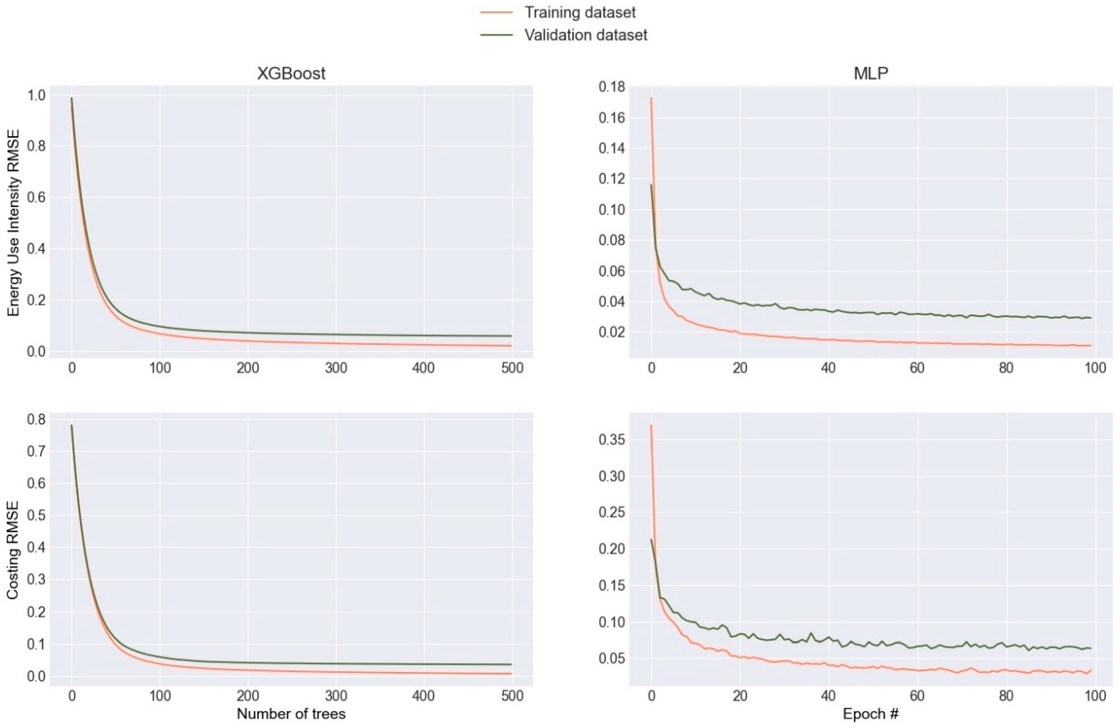
The XGBoost and MLP models for predicting both EUI and costing were trained using 2000 generated buildings by the LHS model with the RMSE as the loss function to minimize error. Additionally, the models’ performance was evaluated using multiple metrics, including MAE and the R².

Figure 3 presents the learning curves for predicting EUI and cost estimates using XGBoost and MLP. The curves indicate that the models generalize well, with only a slight tendency toward overfitting. Although the validation error for all models is slightly higher than the training error, the gap remains minimal, suggesting a well-balanced model. Additionally, based on the learning curve, XGBoost tends to overfit less compared to MLP. It is important to note that the RMSE values in Figure 3 are calculated based on scaled data, as described in the methodology section (using standard scaling).

4.3. Testing Performance

The performance of the trained models was evaluated on the testing dataset using the R², RMSE, and MAE metrics. All performance metrics were calculated using the unscaled (original) target values to ensure that the reported errors reflect the actual units of measurement. The results are summarized in

Table 3. Correlation and error rate for predicting total energy and costing based on the testing dataset.

	Energy			Costing
Model	R2	RMSE (GJ/m2)	MAE (GJ/m2)	R2	RMSE (CAD/m2)	MAE (CAD/m2)
XGBoost	0.990	0.006	0.004	0.996	5.125	2.933
MLP	0.998	0.002	0.002	0.984	10.088	6.465
RF	0.968	0.011	0.008	0.925	21.937	15.068

. Overall, the MLP and XGBoost models demonstrated the highest accuracy, with R² values above 0.99 for energy prediction and above 0.98 for cost prediction. XGBoost performed slightly better than MLP for cost prediction, achieving the highest R² (0.996) and the lowest RMSE and MAE values for this target. Meanwhile, MLP achieved the highest accuracy for energy prediction, with an R² of 0.998 and the lowest RMSE and MAE values among all models.

Random Forest (RF) had the lowest accuracy among the three models but still provided reasonable predictions. The R² values of 0.968 for energy and 0.925 for cost indicate that RF performed well for energy prediction but struggled more with cost prediction, showing the highest RMSE (21.937 CAD/m²) and MAE (15.068 CAD/m²) among the models. This aligns with the expectation that RF is less effective than MLP and XGBoost in capturing complex relationships in high-dimensional data.

Across all models, predicting EUI was consistently more accurate than predicting cost, as shown by the higher R² values and lower error metrics for energy compared to cost. This suggests that the relationship between the input building features and EUI is more straightforward than the relationship with cost, which may be influenced by additional external factors since an external database is being used for generating costing data for each building in the synthetic database.

In summary, MLP and XGBoost performed best for energy and cost prediction, respectively, while Random Forest, despite its lower accuracy, still provided reasonable estimates.

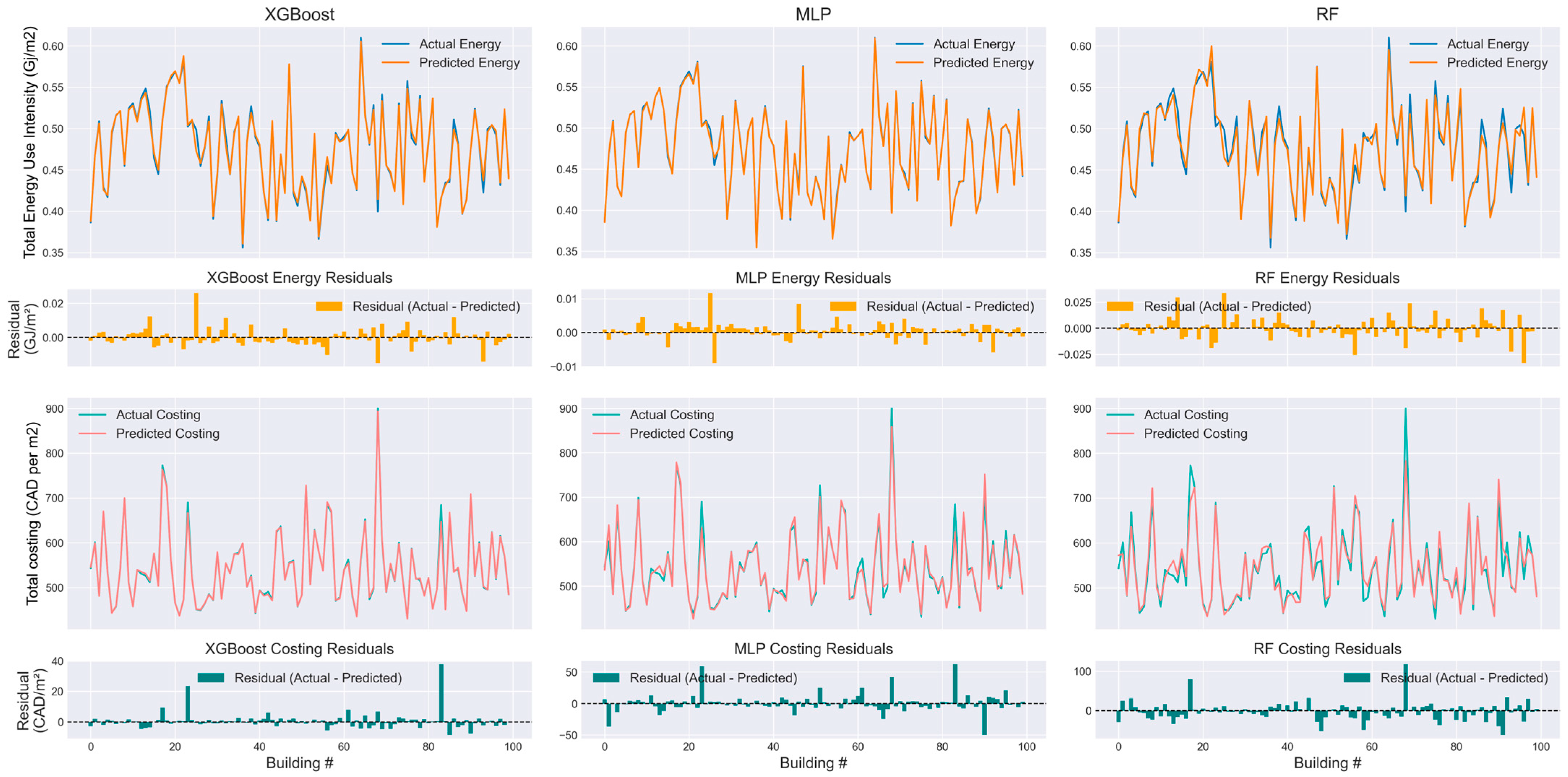
Figure 4 illustrates the performance of XGBoost, MLP, and RF in predicting energy use intensity and cost for 100 unseen buildings from the test dataset. The actual values are compared against the predicted values to assess the models’ accuracy.

XGBoost demonstrates superior performance in predicting building costs, especially for buildings with the highest and lowest costs, where the predicted values closely follow the actual ones. MLP also provides reasonable predictions but shows higher deviations for extreme values, while Random Forest exhibits the most noticeable difference between predicted and actual values, indicating less accuracy in cost estimation.

While all three models perform well in predicting EUI, MLP slightly outperforms the others by maintaining a close alignment between actual and predicted values. XGBoost also provides competitive results, whereas RF displays higher variance, suggesting that it may not generalize as well for energy prediction.

The results align with the testing performance metrics discussed earlier, reinforcing that XGBoost is the best-performing model for cost estimation, whereas MLP is slightly better for energy estimation. The visualization also highlights how RF is less stable, particularly for cost predictions, as its predictions deviate more from the actual values.

4.4. Performance Comparison

The training times of the machine learning models were compared using the same computer, as specified in

Table 4. Hardware specifications used for training, tuning, and testing the ML models, as well as running the physics-based simulation model.

Component	Specification
CPU	Intel i9-13950HX
GPU	Nvidia RTX 2000 Ada Laptop GPU
RAM	64 GB
Storage	1 TB

, with the results presented in

Table 5. Training time in minutes.

Model	Energy (min)	Costing (min)
XGBoost	0.83	0.08
MLP	45.74	0.42
Random Forest	0.93	0.04

.

The MLP model requires significantly more training time compared to the XGBoost and Random Forest models, taking about 46 min for training the energy model and 0.42 min for training the costing model. In contrast, both XGBoost and Random Forest perform much faster, completing the training time in less than a minute for both the energy and costing models. Although XGBoost and Random Forest models take significantly less time to train compared to the MLP models, the prediction accuracy for EUI using the MLP models is higher than the Random Forest and XGBoost models, based on Table 3.

Overall, XGBoost performs the best when considering the accuracy and training time. It offers the same or better accuracy compared to MLP and takes significantly less time to train, similar to Random Forest.

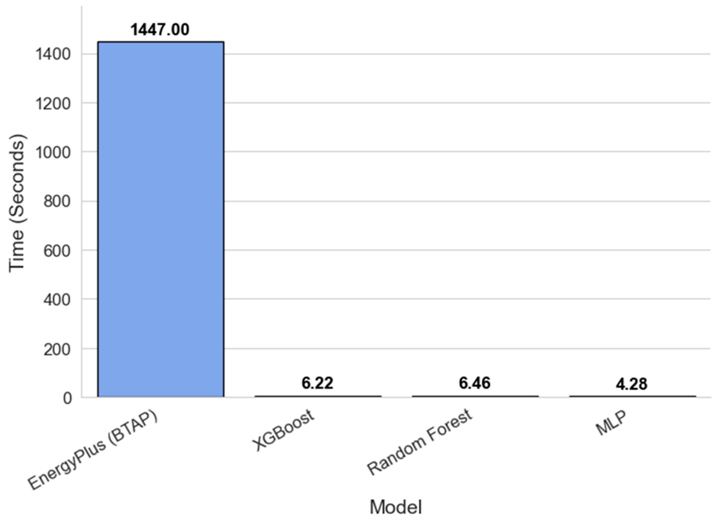
To evaluate how surrogate modeling can improve computational efficiency in calculating the impact of different building feature configurations on energy usage, the time required to process 100 different building configurations and the prediction time were recorded for all three machine learning models and compared to EnergyPlus.

For EnergyPlus, the BTAP tool was used to automatically generate different building configurations using a Python (version 3.13) script, which were then simulated using OpenStudio (version 3.7.0), which runs the EnergyPlus engine. Automating this process eliminates the manual effort of modifying the physics-based model for each configuration, ensuring a fair comparison.

Despite this automation, as shown in Figure 5, the simulation model remains significantly slower, taking up to 340 times longer than the MLP models. In contrast, all three ML models generated results in less than 10 s, not only for energy usage predictions but also for cost estimations—an aspect that the physics-based simulation model does not provide by default.

All models (both ML-based and physics-based simulations) were run on the same computer, whose configuration is summarized in Table 4.

4.5. Impact of Training Size

The size of the training dataset impacts the performance of machine learning models. While larger datasets generally improve model accuracy, they also increase training time. To determine the optimal balance between accuracy and computational cost, training sizes of 500, 1000, 2000, 3000, and 4000 samples were tested.

As shown in Figure 6, XGBoost exhibits relatively stable RMSE values for the energy prediction task as training size increases, suggesting early convergence and limited benefit from additional data. In contrast, the MLP model shows a significant reduction in RMSE, particularly between 500 and 2000 samples, indicating higher sensitivity to training size. Random Forest shows moderate RMSE improvement across all sizes.

For the costing model, all three models show steady reductions in RMSE with increased training data, with XGBoost consistently outperforming the others. Regarding training time, MLP incurs a substantially higher computational cost, which increases almost linearly with training size. In contrast, XGBoost and Random Forest maintain significantly lower training times in the costing model, showing minimal sensitivity to training size in terms of runtime.

Overall, while RMSE decreases and training time increases with larger datasets, there is a threshold beyond which the rate of error reduction slows significantly, while computational cost rises exponentially. This threshold, which represents the optimal training dataset size, is approximately 2000 building samples for both energy and costing models across all three algorithms.

4.6. Design Configuration Analysis and Challenges

To evaluate the capability of the developed surrogate models in assessing different building configurations, a parametric analysis was conducted using one specific building parameter, window thermal conductance. A base building was selected and duplicated ten times, with the only variation across the samples being the window thermal conductance value. In other words, all other building characteristics remained constant, isolating the effect of this single parameter. These modified inputs were then fed into the surrogate models—specifically, the MLP model for energy prediction and the XGBoost model for cost prediction, as they demonstrated superior performance in their respective tasks.

Figure 7 presents a parametric sensitivity analysis showing the influence of window thermal conductance on predicted total electricity energy use, envelope cost, heating, cooling, and ventilation costs. The top subplot displays the distribution of training data for this feature, while the bottom subplot illustrates the predicted performance outcomes across the range of conductance values (W/m²·K).

As expected, a general increase in window thermal conductance—which indicates less thermally resistant windows—correlates with higher total energy consumption due to greater heat loss. At the same time, the envelope cost decreases with higher conductance, reflecting the use of less expensive, lower-performance window assemblies.

However, certain ranges—specifically between 1.6 and 2.1 and beyond 2.4 W/m²·K, show little to no change in predicted total energy. One possible explanation is the distribution of training data used in the machine learning models. As shown in Figure 7, there is a noticeable lack of data samples within these thermal conductance ranges, particularly around 1.6 and 2.4 W/m²·K, compared to a denser distribution near 2.2. This suggests that to improve model sensitivity and predictive accuracy across the entire range of interest, the training dataset should include a more balanced distribution of window thermal conductance values, enabling the model to better learn complex relationships and produce more reliable predictions in previously underrepresented regions.

Another important aspect of understanding machine learning model behavior is the evaluation of feature importance, which provides insights into the model’s sensitivity to different input variables. As listed in Table 1, the input features consist of both numerical and categorical variables. The categorical variables are transformed through one-hot encoding during the preprocessing stage; therefore, the importance of each class within a categorical feature must be analyzed individually.

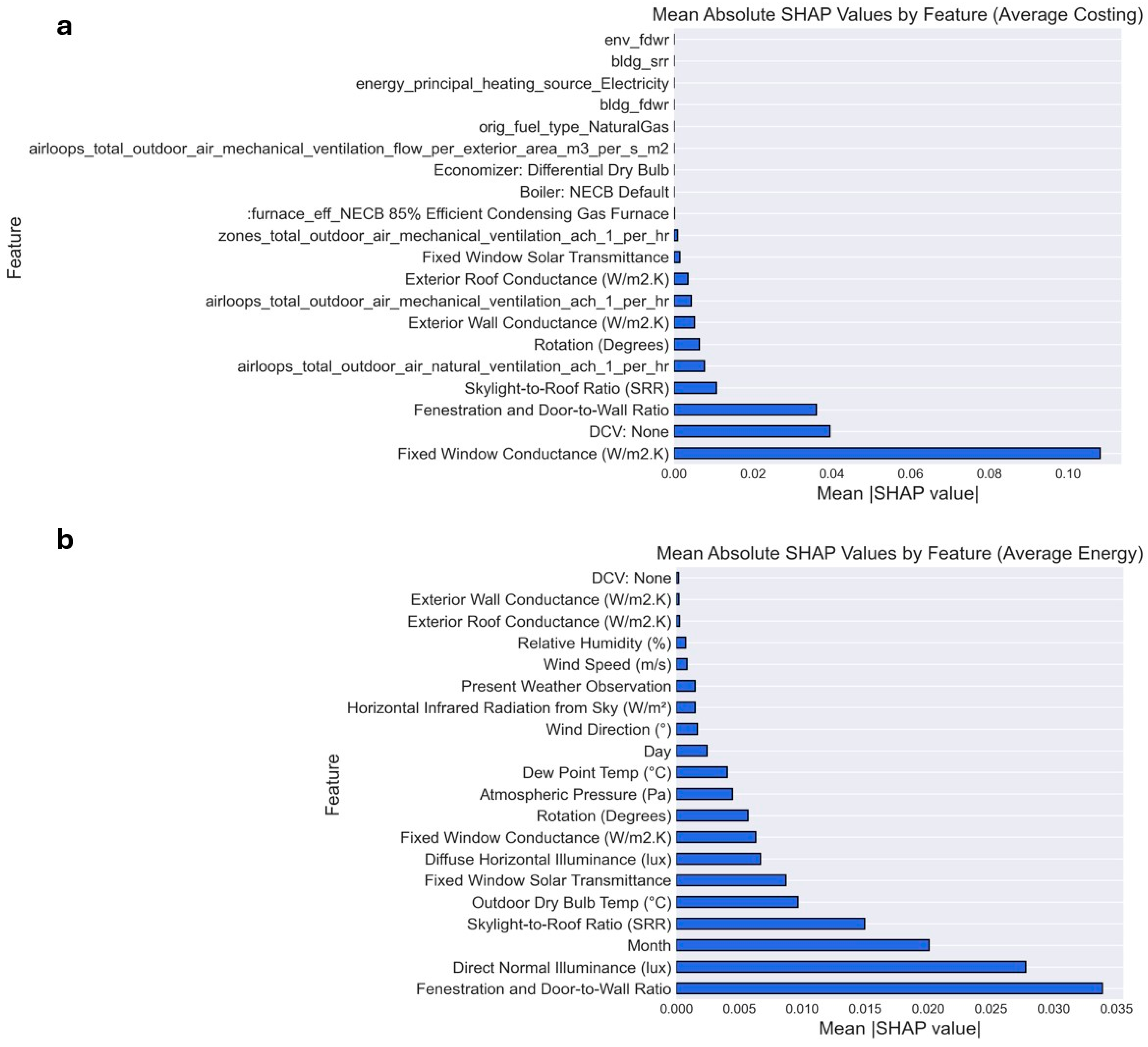
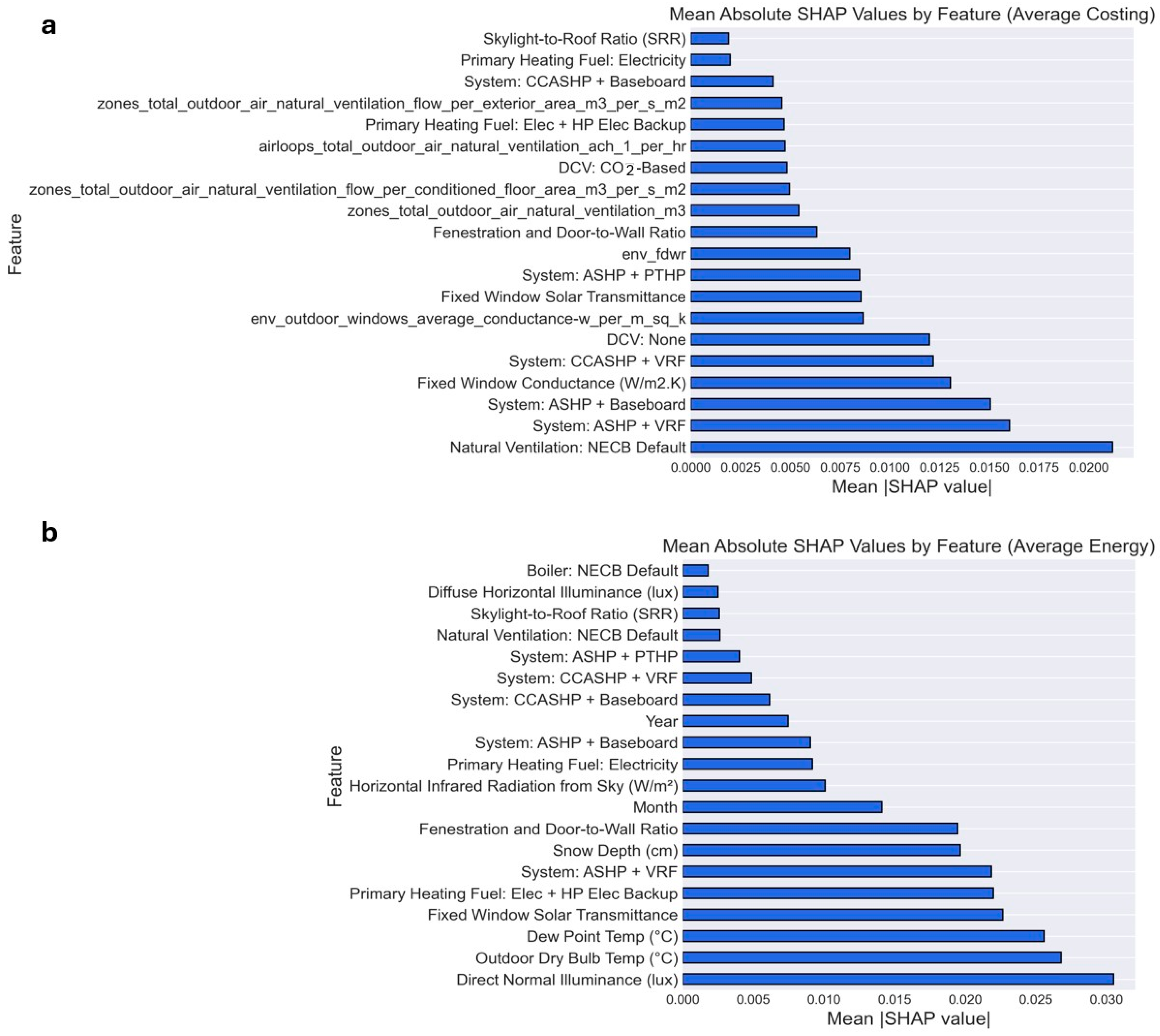
As described in the methodology section, SHAP values were computed for both energy and cost predictions to quantify feature contributions. For the cost prediction task, where multiple output targets exist, SHAP values were averaged across all outputs. The mean absolute SHAP values were then calculated and used to identify the most influential features. These values are presented in Figure 8 and Figure 9 for both XGBoost and MLP models in the context of energy and cost predictions.

The feature attribution was performed using 100 representatives for both models, using all the input building features. Figure 8 and Figure 9 reveal both commonalities and distinctions between the two models. For example, Direct Normal Illumination was consistently ranked as one of the top predictors for energy performance in both XGBoost and MLP, reinforcing its critical role in passive solar gain. However, notable discrepancies also emerged. Dew Point Temperature held greater importance in the MLP model than in XGBoost, potentially reflecting the MLP model’s ability to capture nonlinear humidity-related patterns in thermal performance. Snow Depth similarly appeared among the MLP’s top 20 features for energy prediction but was absent from XGBoost’s ranking—possibly due to differences in how each model handles low-variance or seasonal features.

A particularly insightful difference was observed in Fixed Window Conductance, which ranked highly in XGBoost but was not considered important by MLP. This divergence aligns with findings in Section 4.6 and Figure 7, where the MLP model exhibited a muted response to changes in window properties, suggesting a lower sensitivity to fenestration-related parameters.

Notable differences also emerged in the feature rankings for cost prediction. While both models highlighted key cost-related inputs—such as System Type and Envelope Conductance—the XGBoost model placed greater emphasis on features like Exterior Wall and Roof Conductance. These elements were less influential in the MLP model’s ranking, likely due to XGBoost’s ability to capture complex, piecewise-linear interactions between structural parameters and equipment costs. In contrast, the MLP model assigned higher importance to HVAC system types and ventilation cost, suggesting a stronger sensitivity to mechanical system configurations rather than envelope characteristics.

These variations in feature attribution highlight fundamental differences in how the two model architectures process the input space. MLP models, while capable of capturing complex nonlinear relationships, often require more data to produce stable and interpretable feature importance rankings. In contrast, XGBoost, as a tree-based algorithm, typically yields more consistent and robust SHAP outputs even with smaller datasets. The SHAP analysis provides a more reliable comparison of the models’ internal logic and emphasizes how each architecture prioritizes different design parameters in cost and energy prediction tasks.

4.7. Discussion

The application of machine learning (ML) surrogate models in early-stage building design has been well explored in the literature, particularly for energy performance prediction. However, this study advances the field through several novel contributions that differentiate it from previous research and respond to key limitations identified in the existing body of work.

First, while earlier studies often focus exclusively on energy use or thermal comfort metrics, the current work integrates energy and component-level cost prediction within a single surrogate modeling framework. By generating detailed cost estimates for major systems, including envelope, HVAC, lighting, and domestic hot water, directly from simulation-based training data, this study eliminates the need for post-processing or third-party cost databases, addressing a significant gap noted in recent literature.

Second, the impact of training dataset size is explicitly evaluated, an area that has received limited attention in previous studies, where fixed dataset sizes are commonly assumed. Our findings demonstrate that a relatively modest training set (~2000 samples) can yield reliable results for both energy and cost prediction, offering practical guidance for scalable surrogate model development in time-constrained design workflows.

Third, the integration of SHAP-based model interpretability provides deeper insights into the decision-making logic of different ML algorithms. While SHAP has been employed in prior building energy modeling works, its combination with parametric design sensitivity analysis is uncommon. This study shows how SHAP analysis reveals the different prioritizations of input features by XGBoost and MLP, enriching the understanding of model behavior and supporting more transparent model adoption by practitioners.

Finally, the case study, focused on a midrise residential building in Toronto—was selected due to the building type’s relevance to Canadian urban housing and retrofit initiatives. Although this narrows the scope of direct applicability, the methodological framework is generalizable across other building types and climate zones given appropriate input data.

In summary, this work distinguishes itself through its simultaneous prediction of energy and cost, explicit training efficiency analysis, and multi-level model interpretability, contributing a practical and explainable ML tool for early-stage building design. These aspects collectively support more informed, rapid, and integrated decision-making—an essential capability in modern sustainable design practice. Although the study does not directly implement a decision-support system, the surrogate models developed and evaluated here are well suited for that purpose. They can rapidly assess a wide range of design alternatives, helping designers and decision-makers identify favorable configurations early in the design process, when adjustments are more feasible and cost-effective.

5. Conclusions

This study demonstrates the effectiveness of machine learning-based surrogate models in predicting both EUI and cost estimates for midrise apartment buildings in the Toronto area. Three machine learning algorithms, RF, XGBoost, and MLP, were evaluated based on accuracy, computational efficiency, and scalability. All models exhibited strong predictive performance, with R² values exceeding 0.9 for both EUI and cost estimation. Among them, XGBoost achieved the lowest RMSE for cost prediction, while MLP performed best for EUI prediction.

A key advantage of surrogate models is their ability to directly estimate building costs, something traditional physics-based simulation models do not inherently provide. While physics-based models excel at simulating energy performance, they require separate cost estimation tools and extensive manual input to assess financial impacts. The proposed machine learning models address this limitation by integrating both energy and cost predictions, offering a more efficient and holistic decision-support tool during the early stages of building design.

The computational efficiency of the models was also assessed, showing that all three machine learning models drastically reduced prediction time compared to the baseline physics-based simulation. While MLP required a longer training time, it achieved the fastest prediction time among all models. Furthermore, an analysis of training dataset size showed that model performance improves with more data up to a saturation point, around 2000 samples, beyond which the error reduction is marginal while training cost increases significantly.

To evaluate how these models perform in analyzing different building design configurations, a parametric study was conducted focusing on one key design parameter: window thermal conductance. The models were used to predict energy and cost outcomes for identical building configurations, varying only this parameter. The results demonstrated consistent trends aligned with domain expectations, such as increasing energy use with higher window conductance and decreasing envelope costs. However, certain parameter ranges showed insensitivity in predictions, likely due to sparse data in those intervals, underscoring the need for a more uniformly distributed training dataset.

To further interpret model behavior, SHAP analysis was applied to quantify the contribution of each input feature to the model predictions. This analysis revealed the most influential features in energy and cost prediction and highlighted differences in how XGBoost and MLP models interpret input data. Some features were important in one model but not the other, which may be partially attributed to differences in SHAP sample sensitivity, especially for the MLP model, which may require a larger number of samples for stable interpretation.

Overall, this research highlights the potential of machine learning-based surrogate models as practical and scalable alternatives to traditional simulation tools. These models not only enable rapid predictions but also support integrated energy and cost analysis, improving early-stage decision-making in building design.

Nevertheless, this study has several limitations. The models are trained entirely on synthetic data generated from simulations, which may reflect assumptions or simplifications that do not fully capture real-world conditions. This includes potential biases introduced by modeling choices, input assumptions, and cost estimation parameters. Moreover, the surrogate models were developed for a specific building typology (midrise apartments) and climate zone (Toronto). As such, generalizing the results to other building types or climatic regions would require additional retraining and validation using region-specific data.

Future work should focus on (1) calibrating baseline energy models and incorporating stochastic occupant schedules to improve the realism of synthetic data, (2) exploring more comprehensive building design variations to expand sensitivity analysis, (3) testing the effect of different SHAP sample sizes to enhance the stability and interpretability of feature importance, particularly for neural network-based models like MLP, and (4) investigating the influence of climatic zone heterogeneity by comparing surrogate model performance and optimal training sample sizes across diverse locations (e.g., tropical, temperate, and cold climates). This would help assess the generalizability of model efficiency and data requirements in varied environmental contexts.