Bridge Cable Performance Warning Method Based on Temperature and Displacement Monitoring Data

Abstract

Cable-stayed bridge cables experience significant tension over time, making the bridge cables prone to corrosion and fatigue. The direct measurement of cable length is not a standard capability in most current structural health monitoring systems, nor is long-term monitoring of cable changes. Bridge displacements are caused by both dynamic loads (wind and traffic) and quasi-static factors, primarily temperature. This study filtered out dynamic responses by the three-sigma rule, multiple linear regression, interpolation method, and not-a-number calibration. Monitoring data were used to analyze the bridge’s thermal field distribution and the time-dependent variation of tower displacements. Correlation analysis revealed a strong linear correlation between air temperature and quasi-static tower-girder displacements. This research proposes to use the tower-girder distance (effective cable length) to represent the length of the cable, take the thermal expansion coefficient of the effective length of the cable as the quantitative index for long-term monitoring, and take its error as the performance early warning indicator. This method effectively monitors cable health and provides damage warnings.

1. Introduction

As critical safety components, bridge cables are highly susceptible to degradation in cable-stayed structures, primarily due to prolonged environmental corrosion and progressive material fatigue [1]. Serious casualties and economic losses can result from the collapse of major structures [2,3,4]. Advances in sensing technology are driving the increased adoption of structural health monitoring (SHM) systems to ensure bridge and cable safety [5,6]. Advances in sensing technology have made SHM systems the standard approach for safeguarding bridge and cable safety [7,8,9]. Thermal effects represent a significant environmental load for large civil engineering structures. Analyzing this data to create performance alerts for critical elements like bridge towers is vital for safeguarding operational safety and structural integrity throughout their service life [10,11]. Thermal effects represent a significant environmental load that must be considered in the design of major civil engineering structures [12]. Therefore, the variability of thermally induced quasi-static cable displacements must be analyzed.

The monitoring method of the length of bridge cables is crucial for ensuring the safety of the bridge cables. The vibration-based structural damage detection method, which is widely used in the civil engineering field, is also applicable to the detection of bridge cables [13]. Zhang et al. [14] reviewed the traditional methods for monitoring the force of bridge cables and the innovative methods for monitoring cables, especially the emerging intelligent monitoring methods in recent years. Jin et al. [15] have developed a fully automatic peak value acquisition method for stay cables (a bridge cable monitoring method based on vibration). Wang et al. [16] developed a non-contact visual monitoring system based on computer vision technology by using industrial cameras equipped with infrared filters and infrared light sources and applied it to the tension monitoring of cable-stayed bridge cables.

To monitor bridge temperature changes, the system employs various sensors, necessitating the analysis of the thermal action’s quantitative values and spatial distribution. Lin et al. [17] calculated the maximum and minimum average effective temperatures for parallel side-by-side box girders in a deck extension bridge, based on historical extremes across 12 Chinese cities in four climate zones. Zhu et al. [18] studied a large-span steel truss arch bridge with spherical bearings, accurately mapping its temperature response by incorporating both the bearing performance and spatial temperature variations. Xu et al. [19] studied temperature differentials in steel truss girder bridges. They employed a virtual bridge health monitoring system for detailed temperature difference analysis and used finite element simulations to identify the causes of significant temperature variations. Xia et al. [20] used measured air temperature and solar radiation as thermal boundary conditions. They calculated the solar radiation incident on each external surface at different times and dates using the hemisphere method to determine view factors between the bridge’s surfaces. Elshoura et al. [21] analyzed 115 bridges featuring diverse structural configurations (span number, beam spacing, and beam type). Based on these analyses and the AASHTO LRFD Bridge Design Specifications (BDSs), they estimated the positive thermal moment at the bearing locations and developed a simplified equation for calculating the corresponding positive constraint moment induced by the vertical temperature gradient.

Analyzing the thermal effect and structural response of bridges is the basis of early warning research. Wang et al. [22] developed a method to quantitatively assess cable damage in real-time using monitoring data analysis, correlation analysis, damage assessment, and verification analysis. Fu et al. [23] proposed an analytical solution for temperature-induced deflection, incorporating internal force balance and boundary conditions. Their approach models the temperature effect as an equivalent load on the beam and evaluates the main beam’s response under four different thermal conditions. Zhu et al. [24] analyzed two years of on-site monitoring data from a 108 m steel truss bridge and proposed a simple general formula, describing how temperature distribution relates to temperature-induced strain. Using deep learning and SHM data, Gong et al. [25] created a model to map temperature to strain and predict temperature-induced strain. Zhu et al. [26] presented a method for simulating the effects of solar-induced non-uniform temperature fields in truss suspension bridges. It uses thermal analysis-derived node temperatures as boundary conditions to model resulting structural deformations.

After removing environmental influences, studies on bridge damage warning systems can proceed. Li et al. [27] developed an early warning method for detecting abnormal cable forces in cable-stayed bridges that incorporates the influence of structural temperature. Their approach establishes a baseline model characterizing the typical relationship between healthy cable forces and structural temperature. Abnormalities are detected by identifying deviations between measured cable forces and the forces predicted by this baseline model. Yang et al. [28] proposed cable force characterization vectors to represent cable group behavior and developed an anomaly detection/location method based on changes in these vectors, analyzing the force relationship between adjacent cables under single loading. Chen et al. [29] computationally modeled the continuous collapse of a bridge prototype by simulating the sudden removal of individual stays at various positions and sequential cable removal. Kong et al. [30] conducted a comprehensive review of bridge cable inspection, monitoring, and evaluation, covering common damage types, techniques for detecting surface and internal defects, cable force measurement methods, and condition assessment approaches. Huang et al. [31] created a sparse Bayesian model using long-term SHM data and proposed an early warning method for the temperature and deflection of the main beam.

Current structural health monitoring systems often lack sensors capable of directly measuring cable length variations. While bridge towers are primarily designed as axial compression members, cable damage can induce significant detrimental bending moments. To address thermal loading’s detrimental effects on bridges, this paper introduces a novel performance warning method using errors from an effective cable length model. The paper’s structure is outlined below: first, this study provides an overview of the bridge structure and its monitoring system. Then, comprehensive data preprocessing is carried out using the three-sigma rule, multiple linear regression, interpolation, and not-a-number ($\mathrm{NaN}$) calibration. Second, it investigates temperature variation patterns (air and structural) and displacement correlations between the bridge and its towers. Third, subsequent analysis quantifies the correlations (and their coefficients) between the north tower temperature and air temperature, the south tower temperature and air temperature, and the mid-span displacement at the tower top and air temperature. Fourth, the performance warning method for the effective cable length is validated using monitoring data. Finally, the detailed conclusions are outlined.

2. SHM System and Data Preprocessing

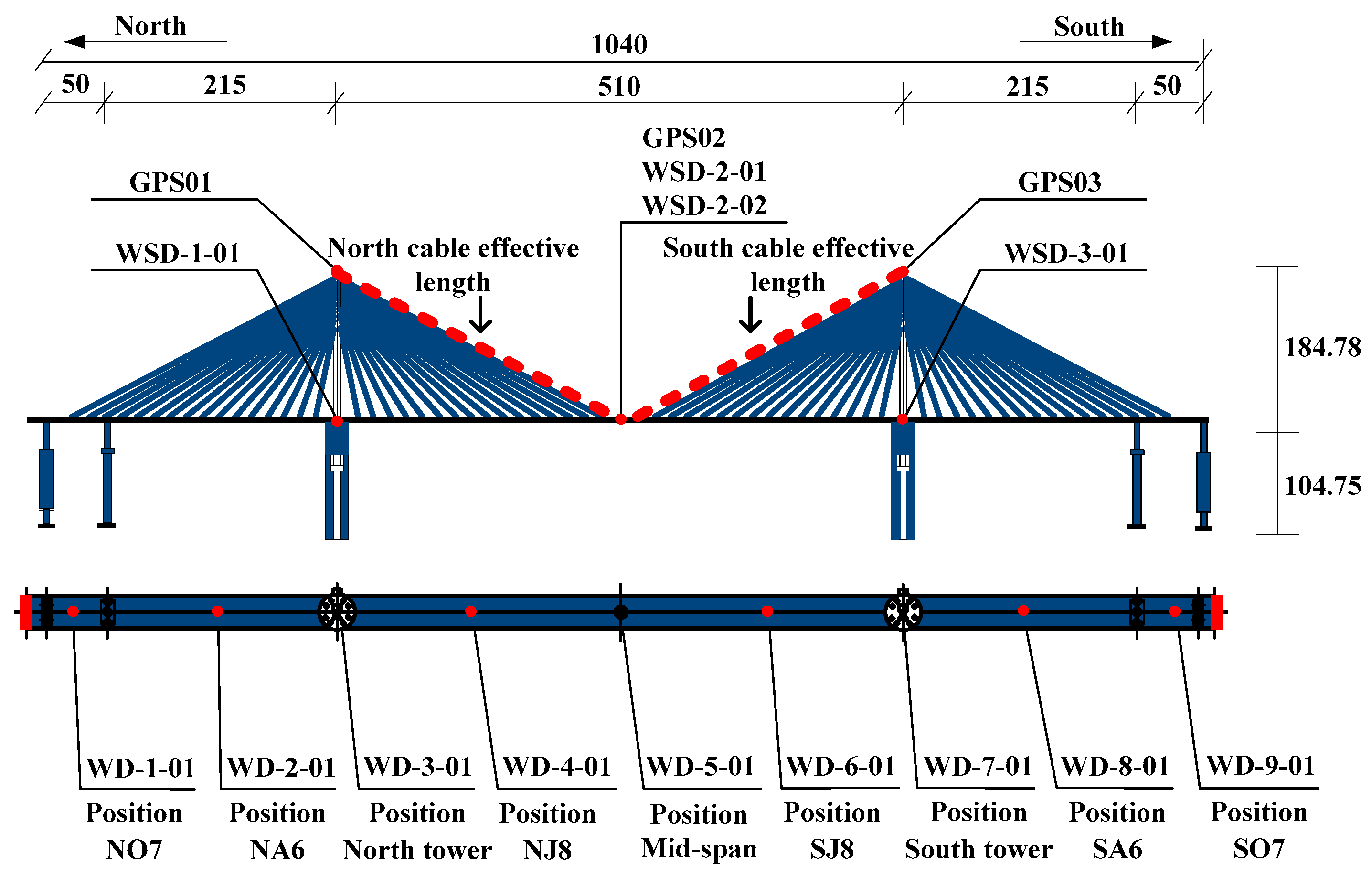
2.1. Overview of the SHM System

Analysis of monitoring data from a symmetrical cable-stayed bridge investigated its thermal field, tower displacements, and tower-girder distances. The Anqing Yangtze River Bridge is a cross-river passage in Anhui Province, China, connecting the Dongzhi County of Chizhou City and the Yixiu District of Anqing City. It is located on the Yangtze River waterway. The 181.53 m tall reinforced concrete cable towers support a bridge deck paved with a 75 mm thick double layer of Stone Mastic Asphalt (SMA) asphalt concrete. Figure 1 and

Table 1. Sensor location and specifications.

Monitoring Subject	Serial Number	Position	Sampling Frequency (Hz)	Unit
Displacement	GPS01	North tower	1	°C
	GPS02	Mid-span	1	°C
	GPS03	South tower	1	°C
Air temperature	WSD-1-01	North tower	1	°C
	WSD-2-01	Mid-span	1	°C
	WSD-2-02	Mid-span	1	°C
	WSD-3-01	South tower	1	°C
Structural temperature	WD-1-01	NO7	1/300	mm
	WD-2-01	NA6	1/300	mm
	WD-3-01	North tower	1/300	mm
	WD-4-01	NJ8	1/300	mm
	WD-5-01	Mid-span	1/300	mm
	WD-6-01	SJ8	1/300	mm
	WD-7-01	South tower	1/300	mm
	WD-8-01	SA6	1/300	mm
	WD-9-01	SO7	1/300	mm

show the sensor layout for the instrumented bridge. Four GR10 GPS sensors produced in Switzerland, sampling at 1 Hz, are installed on the main beams and towers. A total of four air temperature and humidity sensors are installed throughout the bridge. The abbreviation for the temperature and humidity sensor is WSD (Chinese Pinyin abbreviation). Sensors WSD-1-01 and WSD-3-01 are installed in the steel box girders at the base of the north and south towers, respectively. Sensors WSD-2-01 and WSD-2-02 are located at the mid-span and upstream sections of the main beam. This placement at the tower bases and mid-span provides comprehensive monitoring of bridge temperature and humidity changes, adhering to the principle of cost-effectiveness. The sampling rate for all sensors is 1 Hz. Nine structural temperature sensors are installed at nine cross-sections of the entire bridge, namely NO7 (name of the cross-section at the layout position), NA6, north tower, NJ8, mid-span, SJ8, south tower, SA6, and SO7. A structural temperature sensor is installed on the top of the main beam’s steel box girder within each section. The structural temperature sensor is fixed by a custom sensor protection cover and bolts. The sensor protection cover can isolate the interference of air temperature, thereby measuring the structural temperature of the installation site more accurately. The temperature sampling rate of the sensor is 1/300 Hz, and the measurement range is from −30 °C to +85 °C.

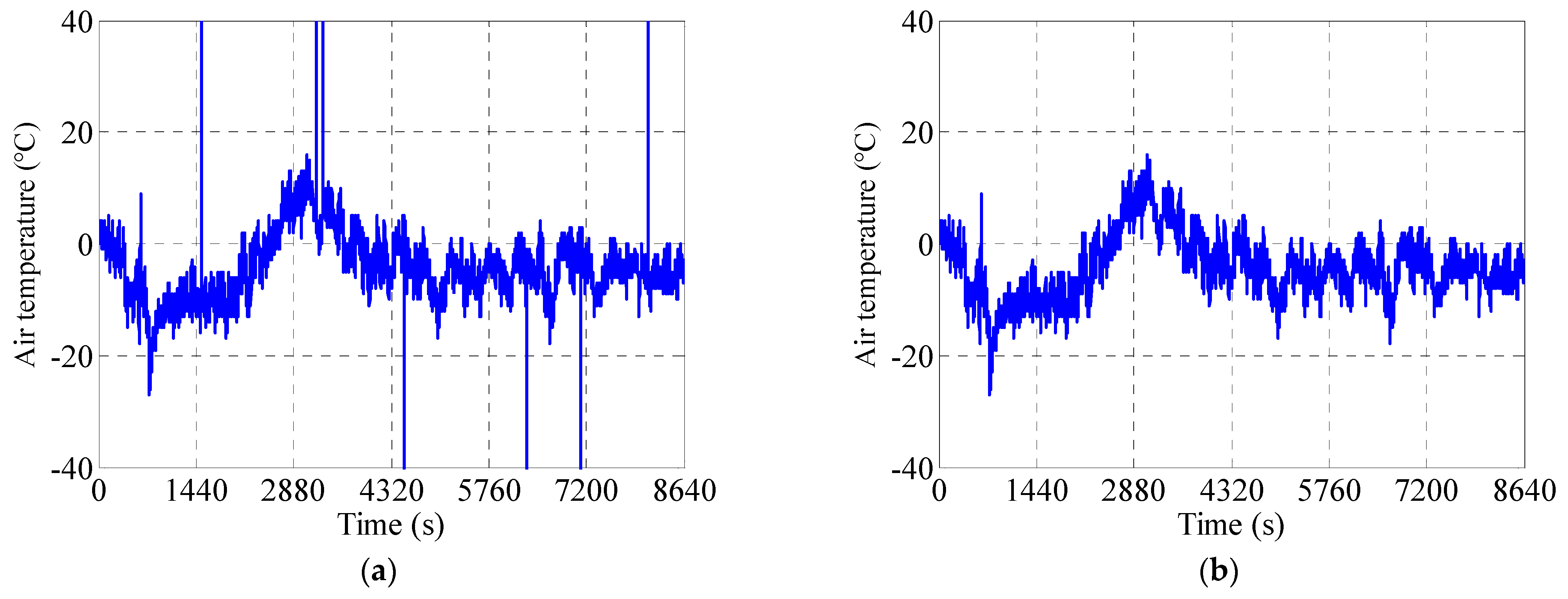
2.2. Method for Skipping Abnormal Monitoring Data

The three-sigma rule method is also applicable for monitoring data where the overall distribution is normal but contains some sporadic large outliers. For a given dataset, let $\sigma$ represent the standard deviation and $\mu$ the mean value. Data points falling within the range $(\mu -a\sigma ,\mu +a\sigma )$ are considered normal, while those outside this range are identified as anomalies. The three-sigma rule method is also applicable for monitoring data where the overall distribution is normal but contains some sporadic large outliers. For a given dataset, let $\sigma$ represent the standard deviation and $\mu$ the mean value. Data points falling within the range $(\mu -a\sigma ,\mu +a\sigma )$ are considered normal, while those outside this range are identified as anomalies. The three-sigma rule approach typically uses k = 3 as the default threshold. Since the skipped abnormal values are much larger than the normal monitoring data, in this paper, the default value of k = 3 can be selected to correct the skipped abnormal values. However, a more appropriate k-value can be determined based on specific data characteristics or empirical practices in monitoring data processing. Figure 2 demonstrates the results of correcting air temperature monitoring data using this method, as follows: Figure 2a shows the original temperature time-history curve containing discontinuous outliers, while Figure 2b presents the corrected curve after three-sigma rule processing. This illustrates that the three-sigma rule method effectively handles discontinuous anomalies in temperature monitoring data.

This approach typically uses k = 3 as the default threshold. Since the skipped abnormal values are much larger than the normal monitoring data, in this paper, the default value of k = 3 can be selected to correct the skipped abnormal values. However, a more appropriate k-value can be determined based on specific data characteristics or empirical practices in monitoring data processing. Figure 2 demonstrates the results of correcting the air temperature monitoring data using this method. Figure 2a shows the original temperature time-history curve containing discontinuous outliers, while Figure 2b presents the corrected curve after three-sigma rule processing. This illustrates that the three-sigma rule method effectively handles discontinuous anomalies in temperature monitoring data.

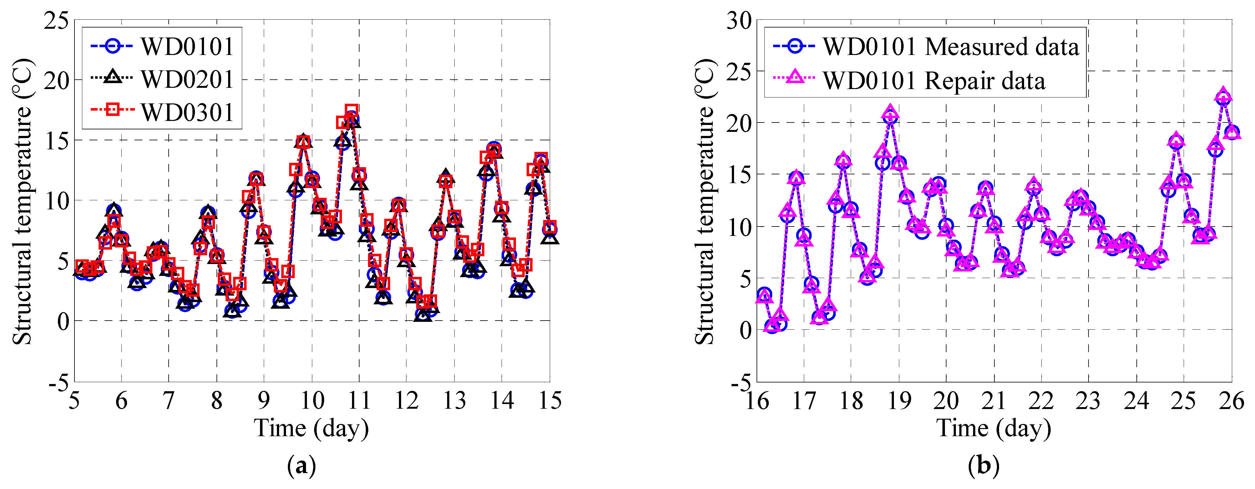
2.3. Method for Missing Abnormal Monitoring Data

2.3.1. Method for Missing Abnormal Monitoring Data Based on Multiple Linear Regression

This method for repairing missing or abnormal monitoring data, based on multiple linear regression, is applicable when data originates from multiple similar sensors. Regression equations are derived for these similar sensors using multiple linear regression. When one sensor fails or has missing readings, the corresponding regression equation can be utilized to estimate the absent data. Assuming a monitoring system employs similar sensors {${\mathit{x}}_1$, ${\mathit{x}}_2$, $\cdots$ ${\mathit{x}}_i$} and the sensor experiencing data loss is ${\mathit{y}}_i$, the regression equation takes the following form:

$${\mathit{y}}_i=b_0+b_1{\mathit{x}}_1+b_2{\mathit{x}}_2+\cdots +b_i{\mathit{x}}_i+u_i$$

(1)

where ${\mathit{y}}_i$ is the variable to be estimated, ${\mathit{x}}_1$, ${\mathit{x}}_2$, $\cdots$ ${\mathit{x}}_i$ are the monitoring data from similar sensors, $b_0$, $b_1$, $\cdots$ $b_i$ are the coefficients of the multiple linear regression equation, and $u_i$ is a random error term.

Figure 3 presents the reconstruction of the missing abnormal temperature monitoring data using multiple linear regression. Figure 3a displays the temperature time-history curve for 5–15 January 2014, showing the monitored data from the structural temperature sensors: WD0101 (section NO7), WD0201 (section NA6), and WD0301 (north tower section). The multiple linear regression model for this case is defined by the equation $y_i=-0.1242+0.8719x_1+0.1400x_2$. Figure 3b shows the regenerated temperature profile for 16–26 January 2014 produced by this model. The calculated WD0101 curve exhibits close correspondence with the empirical data, particularly in matching temporal patterns and fluctuation characteristics. This agreement between regression-estimated values and measured data validates the effectiveness of the multiple linear regression approach for reconstructing incomplete monitoring datasets. The faithful reproduction of the temperature profile over this 10-day period confirms the model’s capability to accurately recover missing structural health monitoring data by leveraging relationships among multiple variables.

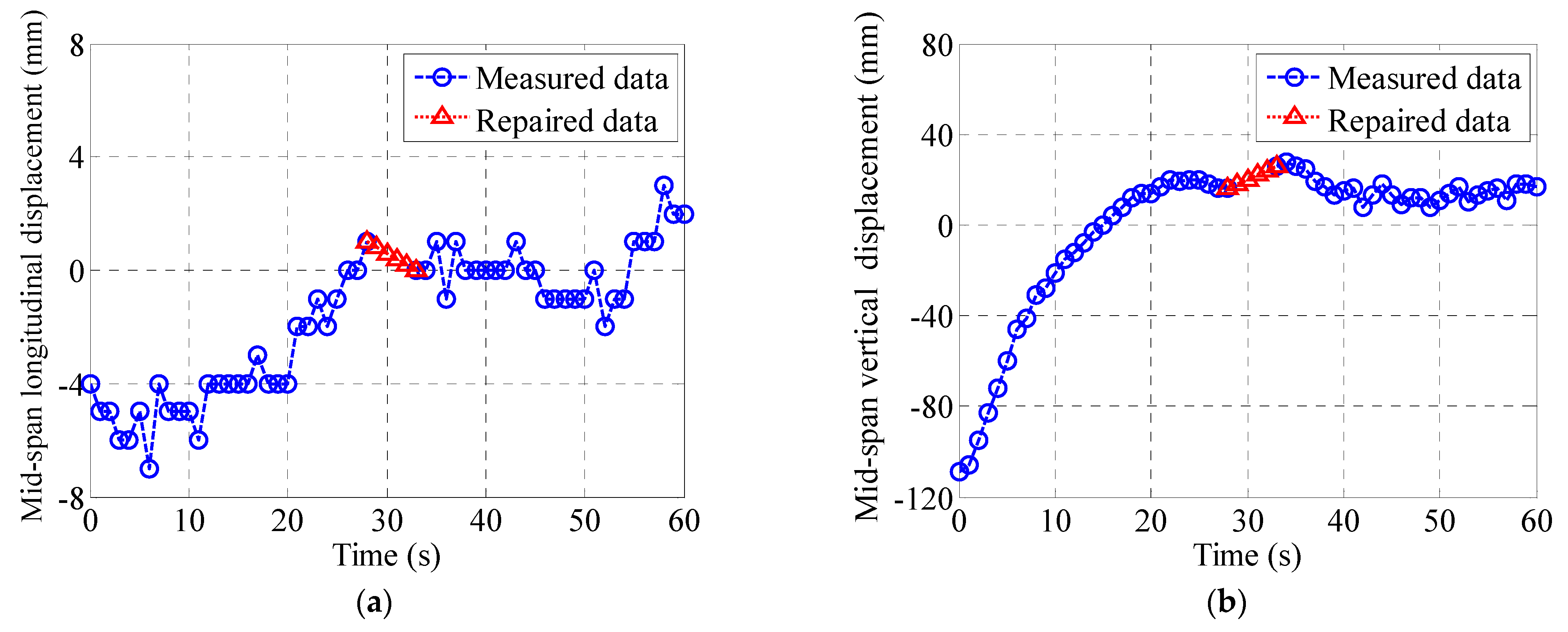
2.3.2. Method for Missing Abnormal Monitoring Data Based on Interpolation Method

The interpolation method for repairing missing abnormal monitoring data is best suited for datasets with limited gaps. It is generally unsuitable for data experiencing large-scale missing values, as extensive repairs can lead to peak loss and can compromise correction accuracy. Figure 4 demonstrates the repair of the abnormal displacement monitoring data using interpolation. In this case, a sensor failure caused a relatively short-duration loss of mid-span displacement, making interpolation viable. Specifically, Figure 4a,b show the interpolation repair results for longitudinal and vertical displacements on 1 June 2014. This illustrates that interpolation can effectively repair monitoring data with minor missing segments, even when no similar sensors are available.

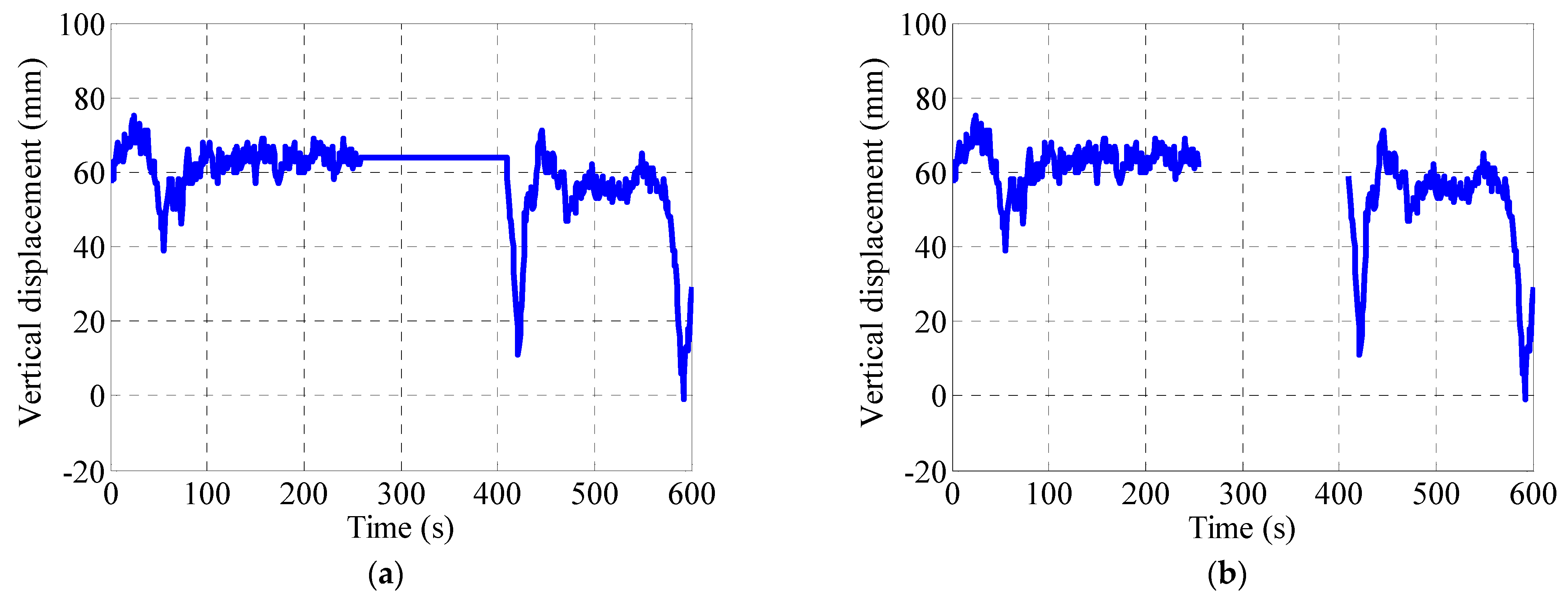
2.4. Method for Constant Abnormal Monitoring Data

Constant anomaly monitoring data refers to the partial data turning into constants due to sensor failure or storage system failure. If there are similar sensors, the multiple linear regression method can be used for repair. If there are no similar sensors and a large number of them are missing, repair cannot be carried out. Constant values can affect the overall mean of the data and the modeling accuracy of other data, so it is necessary to label the constant monitoring data as without data. That is, change the constant part to $\mathrm{NaN}$ for storage. This way, it will not affect the overall mean of the data, nor will it affect the results of modeling with other monitoring data. Figure 5 shows the repair of the displacement constant anomaly in the vertical bridge direction across the middle and lower reaches on 1 February 2014. The number of constant anomaly sampling points is 223, and the 223 constant anomaly monitoring data points are changed to $\mathrm{NaN}$ storage. Figure 5a,b, respectively, show the displacement-time curves of the vertical bridge in the middle and lower reaches before and after displacement calibration.

3. Temperature Environment and Bridge Displacement Response

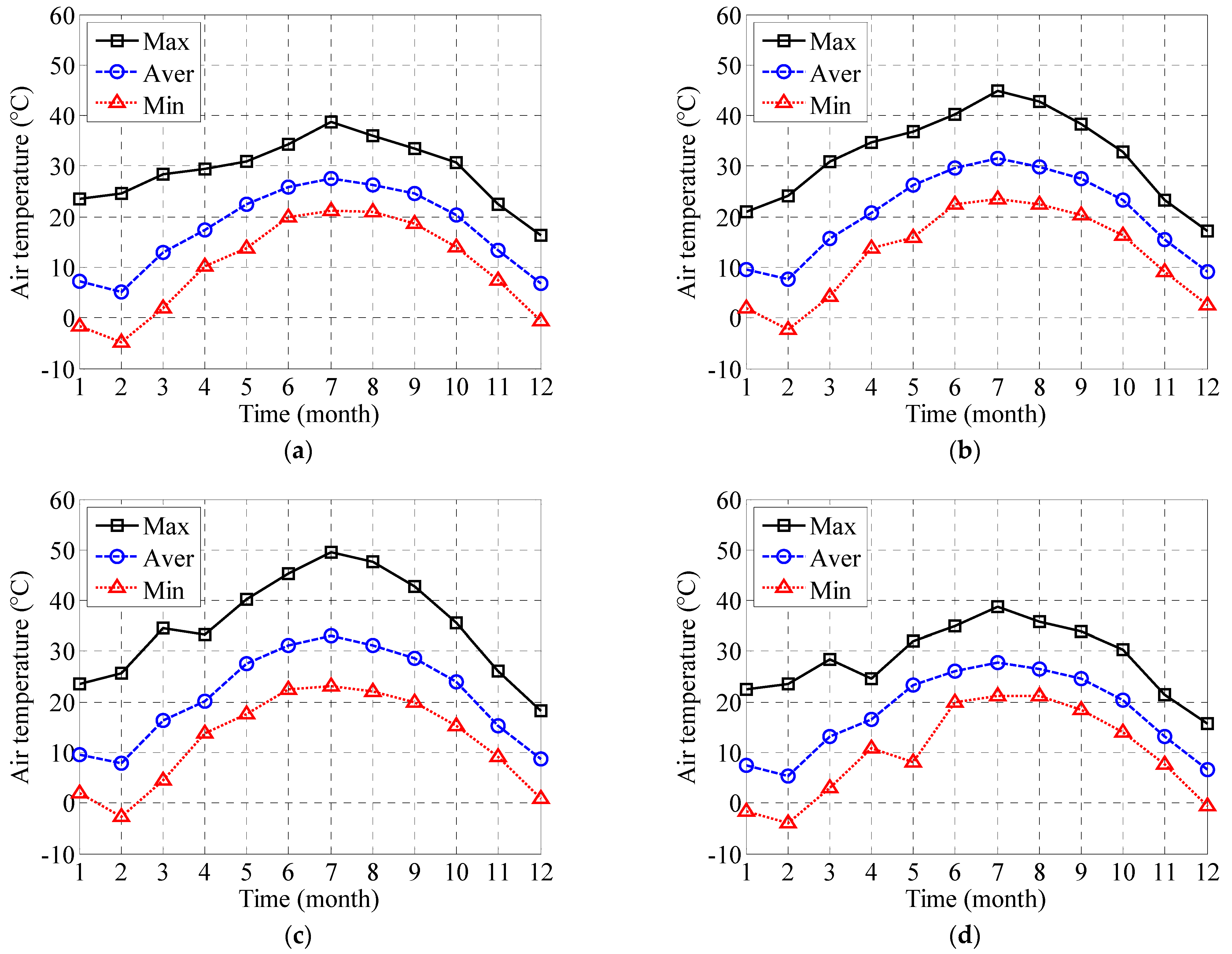
3.1. Air Temperature Time-Varying Law

Figure 6a,d, respectively, show the air temperature variation trends in WSD-1-01 at the bottom of the north tower, WSD-2-01 across the middle and upper reaches of the main beam, WSD-2-02 across the middle and lower reaches of the main beam, and WSD-3-01 at the bottom of the south tower. Figure 6 shows identical trends for the monthly maximum air temperature (square node), monthly average air temperature (circular node), and monthly minimum air temperature (triangular node). Furthermore, by comparing Figure 6a,d, it can be seen that the overall trends for WSD-1-01, WSD-2-01, WSD-2-02, and WSD-3-01 are the same. Since WSD-1-01 and WSD-3-01 are installed in the steel box girder at the bottom of the cable tower, while WSD-2-01 and WSD-2-02 are installed on the main girder, the trend curves of the main beam crossing the middle and upper reaches of WSD-2-01 and the main beam crossing the middle and lower reaches of WSD-2-02 are significantly higher than those of the bottom of the northern tower WSD-1-01 and the bottom of the southern tower WSD-3-01.

Since the air temperature is the highest in July, this section continues to analyze the air temperature time-history curve for July. Figure 7a is the time-history curve of the air temperature in July. From the 10 min average dataset, there are a total of 4464 data points. It can be seen that the curves of WSD-1-01 at the bottom of the north tower and WSD-3-01 at the bottom of the south tower coincide and are within the normal range of air temperature values. The time-history curves of the main beam, spanning the middle and upper reaches of WSD-2-01, are higher than those of WSD-1-01 at the bottom of the north tower and WSD-3-01 at the bottom of the south tower. Furthermore, the trends in the time-history curves of WSD-1-01, WSD-3-01, and WSD-2-01 are all the same. Figure 7b shows the time-history curve of air temperature from July 22nd to 23rd. The daily variation law of temperature can be intuitively observed. By comparison, it can be seen that the curve trends from 0 to 24 points (23rd day) and from 24 to 48 points (24th day) are the same, that is, the daily variation law of air temperature. Furthermore, the air temperatures of WSD-1-01 and WSD-3-01 reached the lowest value around 7 o’clock and the highest value around 4 o’clock, while the air temperature of WSD-2-01 reached the lowest value around 8 o’clock and the highest value around 5 o’clock. These are the differences caused by the influence of high road surface temperature on WSD-2-01.

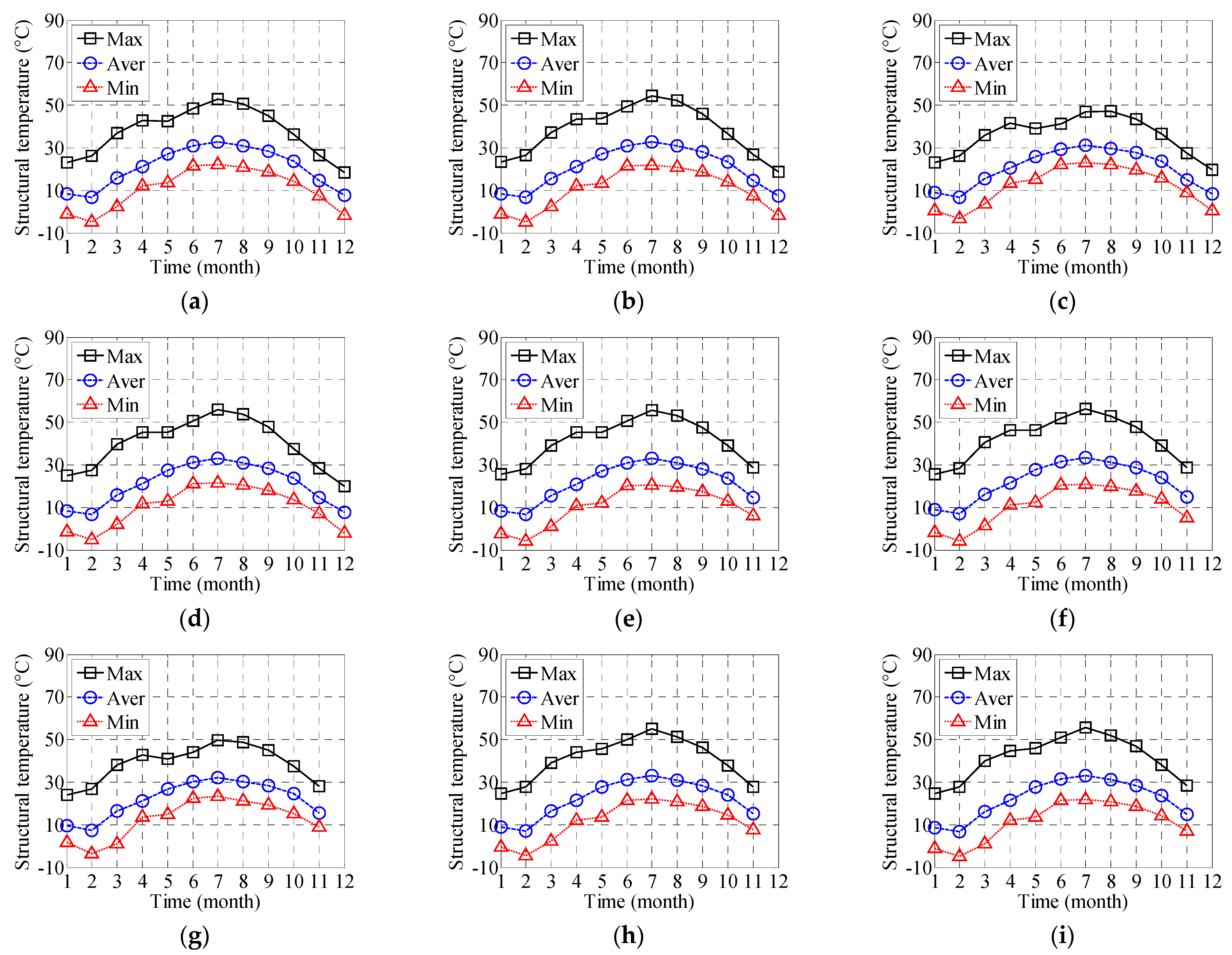
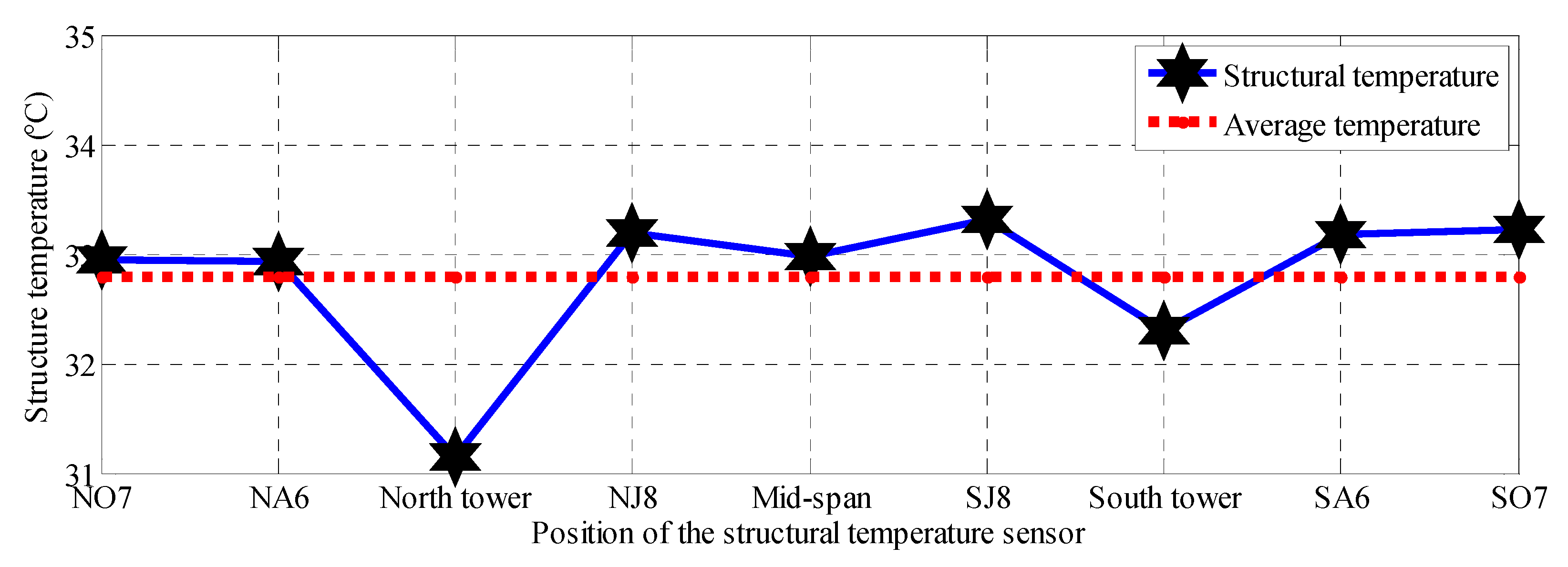
3.2. Structural Temperature Time-Varying Law

There are many structural temperature sensors in the bridge layout, and the temperatures of the upstream and downstream sections of the same section are close. Therefore, this section continues to conduct statistics and analysis on the nine sensors upstream. Figure 8a–i, respectively, show the structural temperature variation trends upstream of the NO7 section (layout position section name), NA6 section, north tower section, NJ8 section, mid-span section, SJ8 section, south tower section, SA6 section, and SO7 section. Among them, the data on the NO7 section, NA6 section, north tower section, and NJ8 section for the whole year of 2014 were not missing, while the data on the middle span section, SJ8 section, south tower section, SA6 section, and SO7 section for December 2014 were missing. It can be seen from Figure 8 that the trends in the monthly maximum structural temperature curves of the square nodes, the monthly average structural temperature curves of the circular nodes, and the monthly minimum structural temperature curves of the triangular nodes are the same. Figure 8a–i show consistent temperature trends across the bridge. However, shadows cast by the towers cause lower temperatures at the north and south tower locations.

Figure 9 is the average structural temperature distribution map of the entire bridge in July 2014. The average temperatures upstream of the NO7 section, NA6 section, north tower section, NJ8 section, mid-span section, SJ8 section, south tower section, SA6 section, and SO7 section in July 2014 were 32.94 °C, 32.93 °C, 31.15 °C, 33.20 °C, 32.98 °C, 33.32 °C, 32.30 °C, 33.18 °C, and 33.23 °C, respectively. The dotted line in Figure 9 shows an average structural temperature of 32.80 °C upstream of the NO7 section, NA6 section, NJ8 section, mid-span section, SJ8 section, SA6 section, and SO7 section. The structural temperature upstream of the north tower section is 1.96 below average, while that of the south tower section is 0.81 below.

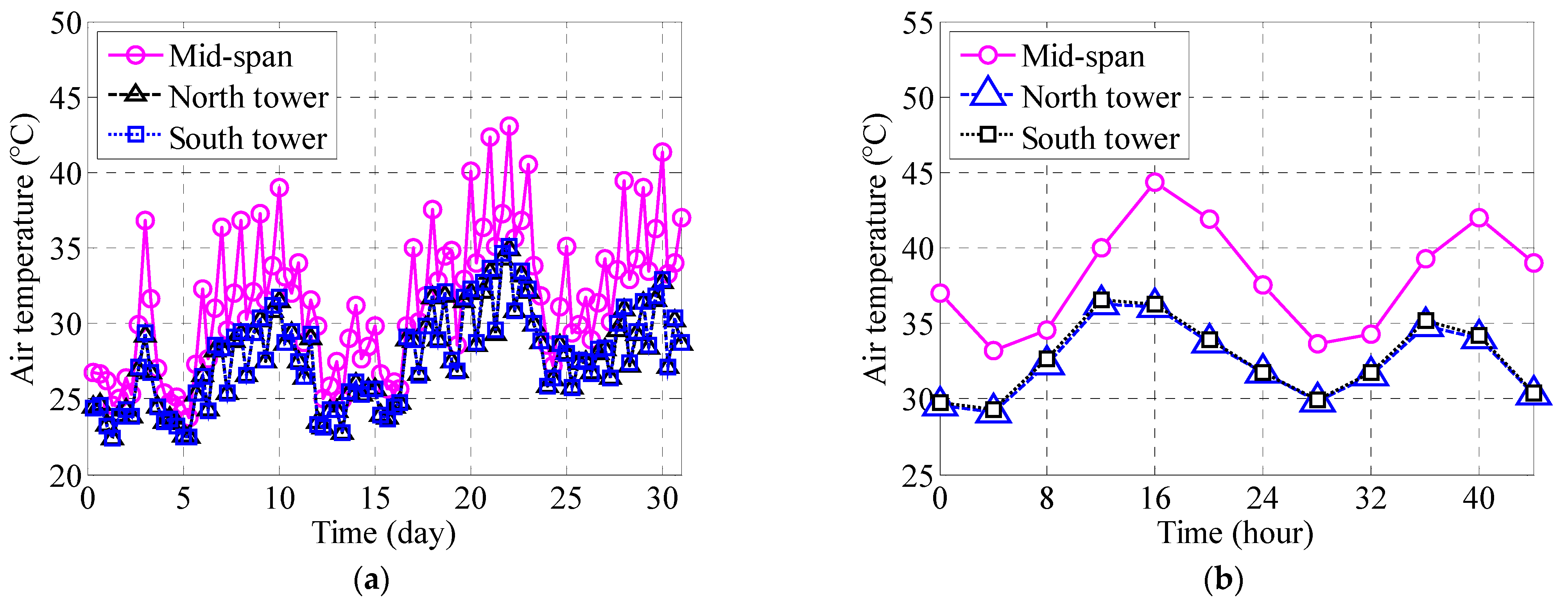
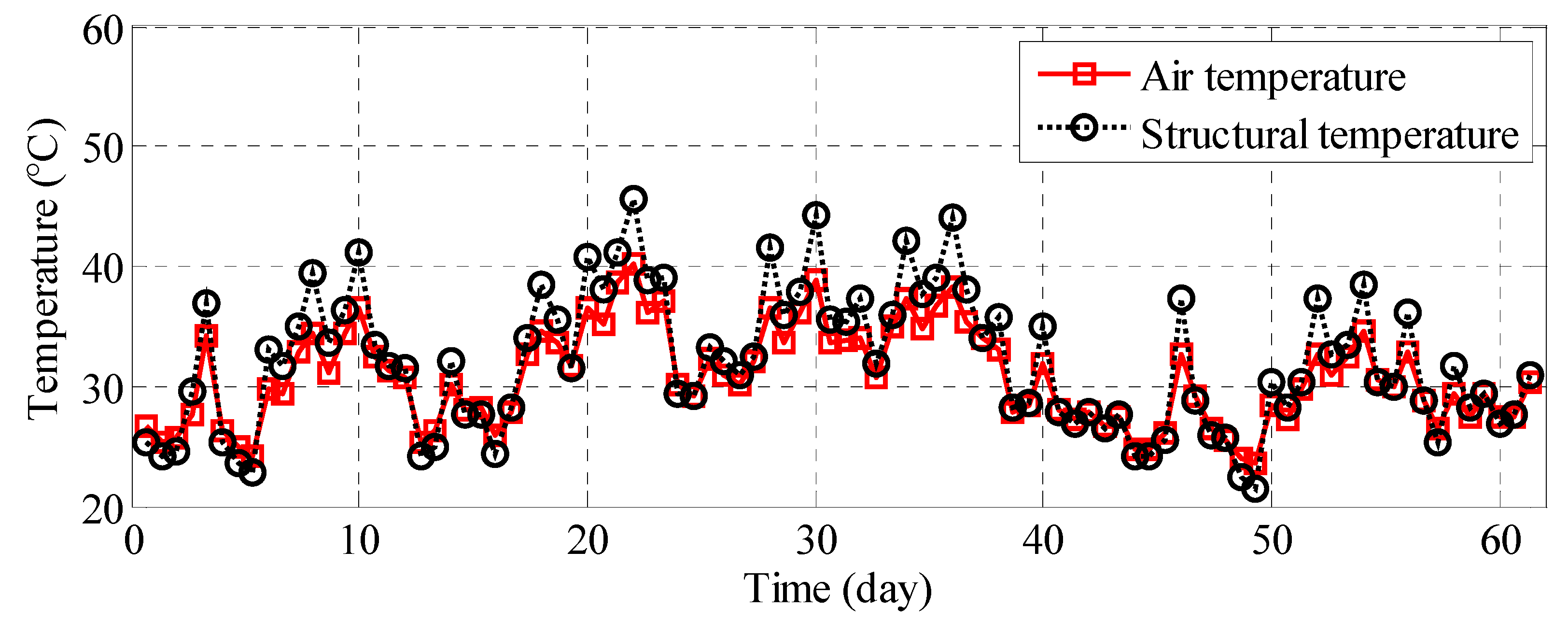
3.3. Air-Structure Temperature Relationship

Sensors measure bridge structure temperature at the north tower, south tower, and mid-span. Figure 10 compares this structural temperature to air temperature for July and August 2014. Maximum structure temperatures significantly exceed maximum air temperatures, whereas minimum structure temperatures are comparable to minimum air temperatures.

3.4. Displacement Response of Bridge Tower

Temperature primarily induces static deformation. To isolate this static component, we averaged the displacement data points over 10 min intervals, effectively filtering out high-frequency dynamic effects caused by factors like wind or highway traffic. Figure 11 presents the June and July 2014 displacement-time curves for the north and south towers. It reveals opposing longitudinal (x-axis) displacement trends between the towers. Although minor fluctuations in the displacement curves (due to residual dynamic effects) contrast with the smoother temperature curves, the primary opposing movement stems from the thermal expansion and contraction of the bridge deck.

4. Temperature-Displacement Statistical Relationship

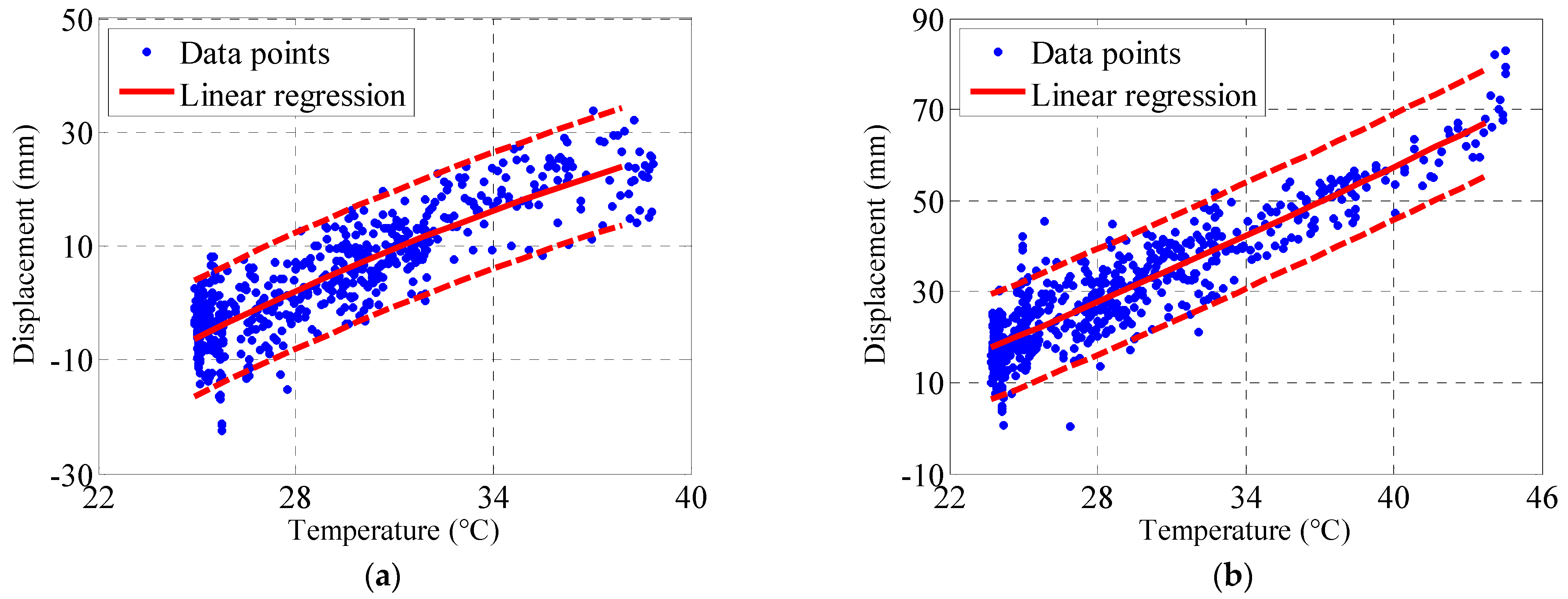
4.1. Temperature-Displacement Statistical Relationship of Bridge Tower

In this paper, air temperature is used instead of structural temperature for cable thermal modeling. As can be seen from the structural diagram (Figure 1), the air temperature sensor is closer to the north-south cables and exposed to the air, which can better represent the temperature of the cable. The structural temperature sensor is installed inside the main beam steel box girder to measure the temperature of the main beam steel box girder. Furthermore, in the structural temperature analysis in Section 3.2 of this paper (Figure 9), it can be seen that due to the shadow occlusion of the north-south cable towers, the structural temperatures of the north-south cable towers are relatively low, which can lead to a large error in the cable thermal modeling. Figure 12 compares the air temperature and tower displacement from 9 to 12 July. Figure 12a shows a strong positive correlation between the air temperature and longitudinal displacement at the north tower. Figure 12b shows the correlation analysis between the absolute value of the longitudinal displacement at the south tower and the air temperature. Figure 13 quantifies this relationship through linear regression analysis of the air temperature versus tower displacement, with the correlation coefficient indicating the strength of the association.

$$R={\displaystyle \frac{{\displaystyle \sum (X_i-\overline{X})(Y_i-\overline{Y})}}{\sqrt{{(X_i-\overline{X})}^2}\sqrt{{(Y_i-\overline{Y})}^2}}}$$

(2)

where $R$ is the correlation coefficient between the structural temperature and tower displacement; $X_i$ and $Y_i$ are the $i\mathrm{th}$ air temperature samples and tower displacement samples, respectively; and $\overline{X}$ and $\overline{Y}$ are the averages of the air temperatures and tower displacement, respectively.

Based on 576 data points (

Table 2. Correlation coefficients for air temperature and tower displacement.

$\mathit{X}$	$\mathit{Y}$	Sample Number	$\mathit{R}$
Air temperature	Displacement of north tower	576	0.87
Air temperature	Displacement of south tower	576	0.91

), the air temperature shows a strong positive correlation (0.87) with displacement at the north tower and a strong positive correlation (0.91) at the south tower. This confirms a strong overall temperature-displacement relationship. The opposing signs indicate the symmetrical displacement behavior of the towers relative to the bridge’s mid-span.

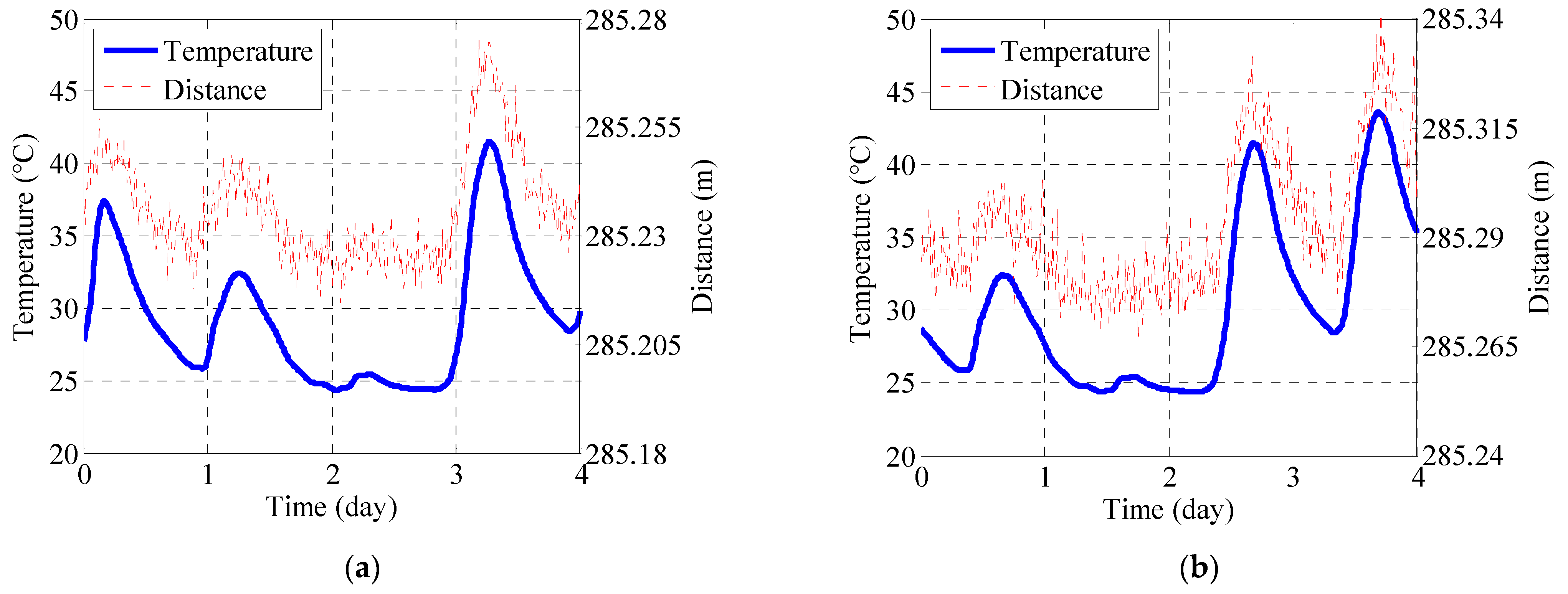
4.2. Temperature-Displacement Statistical Relationship of Tower-Girder Distance

Although bridge cables are critically important, they are rarely monitored directly using sensors. While cable mechanics fundamentally depend on length changes, the distance between the top anchor and mid-span is predominantly driven by temperature fluctuations. Therefore, accurately assessing thermally induced variations in the distance between the tower and the girder is crucial, as this distance directly determines the length of the bridge’s outermost cable. The specific equation governing the distance between the girder and the north tower is:

$${\mathrm{D}}_{ng}=\sqrt{{(x_{ni}-x_{gi})}^2+{(y_{ni}-y_{gi})}^2+{(z_{ni}-z_{gi})}^2}$$

(3)

where ${\mathrm{D}}_{ng}$ is the distance between the north tower and the girder; $x_{ni}$, $y_{ni}$, and $z_{ni}$ are the $i\mathrm{th}$ longitudinal, lateral, and vertical coordinates of the north tower; and $x_{gi}$, $y_{gi}$, and $z_{gi}$ are the $i\mathrm{th}$ longitudinal, lateral, and vertical coordinates of the girder.

The distance between the girder and the south tower is given by

$${\mathrm{D}}_{sg}=\sqrt{{(x_{si}-x_{gi})}^2+{(y_{si}-y_{gi})}^2+{(z_{si}-z_{gi})}^2}$$

(4)

where ${\mathrm{D}}_{sg}$ is the distance between the south tower and the girder; $x_{si}$, $y_{si}$, and $z_{si}$ are the $i\mathrm{th}$ longitudinal, lateral, and vertical coordinates of the south tower; and $x_{gi}$, $y_{gi}$, and $z_{gi}$ are the $i\mathrm{th}$ longitudinal, lateral, and vertical coordinates of the girder.

The temporal variability of air temperature, derived from the mean of sensors WSD-1-01 and WSD-2-01, is compared with the variability of the north tower-girder distance in Figure 14a. Correspondingly, Figure 14b presents a comparison between air temperature variability (the mean of WSD-2-01 and WSD-2-01) and the variability of the south tower-girder distance. Both figures reveal identical changing trends between tower-girder distance and air temperature. This strong linear relationship is further demonstrated in Figure 15 and

Table 3. Correlation coefficients for air temperature and tower-girder distances.

$\mathit{X}$	$\mathit{Y}$	Sample Number	$\mathit{R}$
Air temperature	North tower-girder distance	576	0.94
Air temperature	South tower-girder distance	576	0.93

, which show high correlation coefficients of 0.94 (north) and 0.93 (south). Consequently, the tower-girder distance clearly increases with rising temperatures.

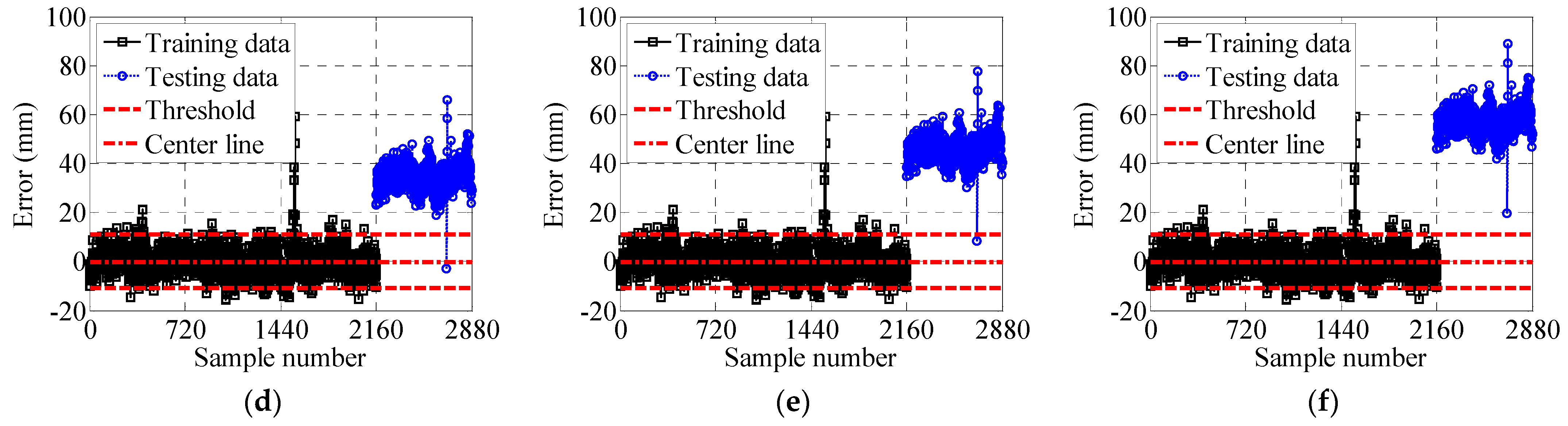
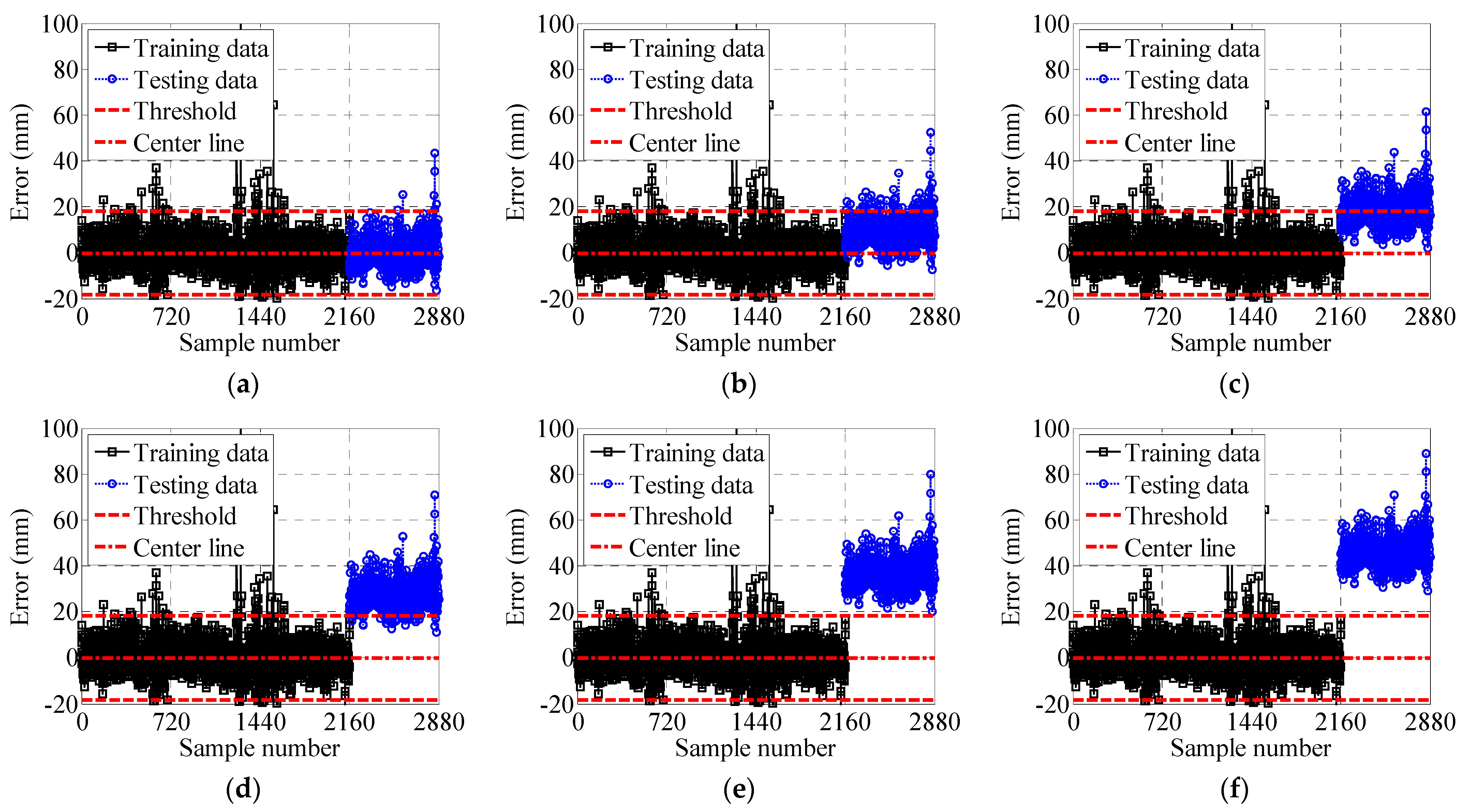
5. Bridge Cable Damage Warning Based on Monitoring Data

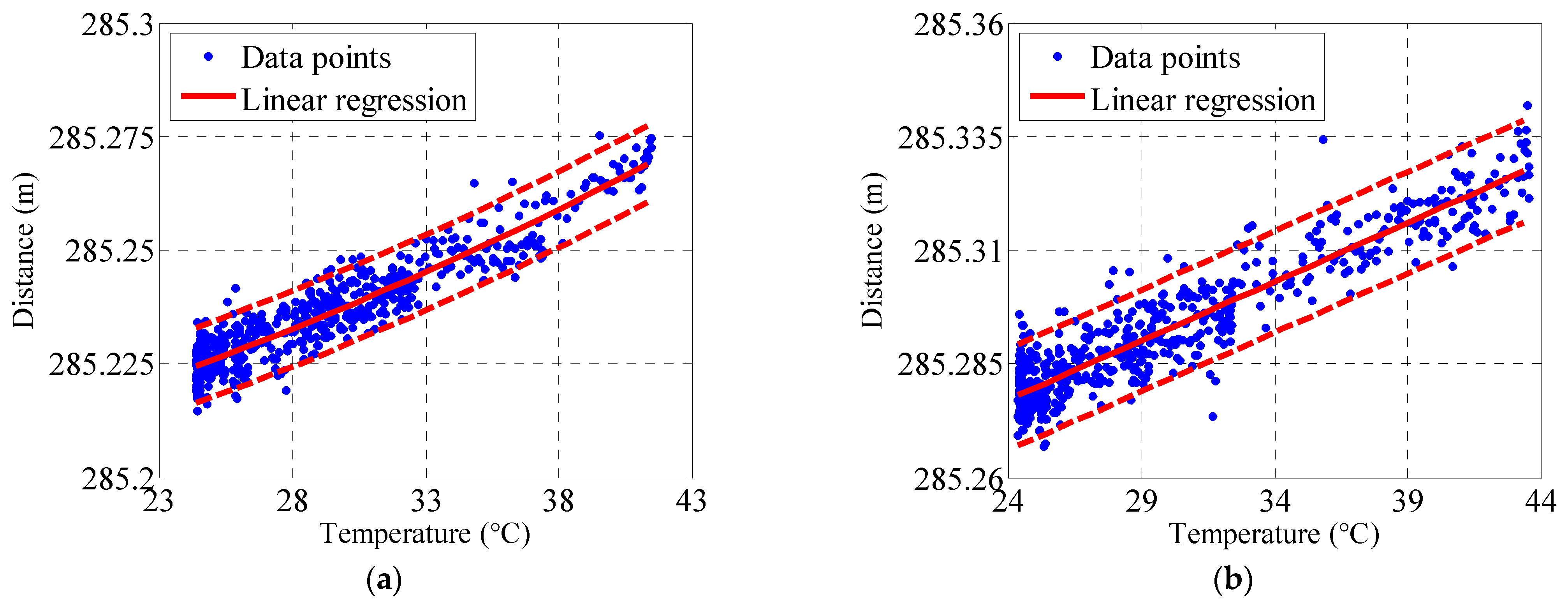
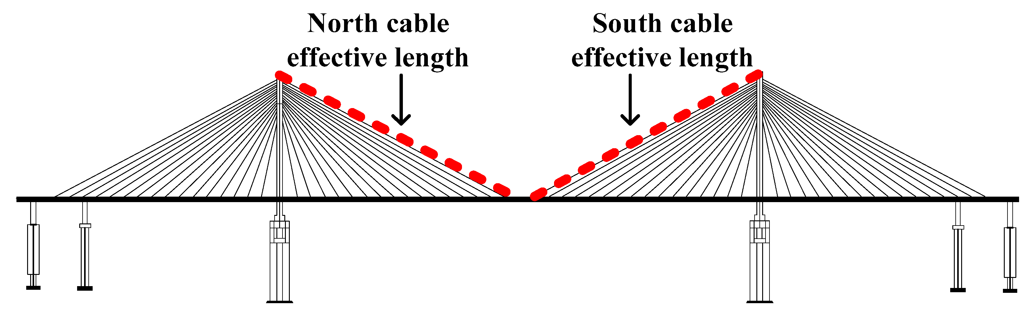
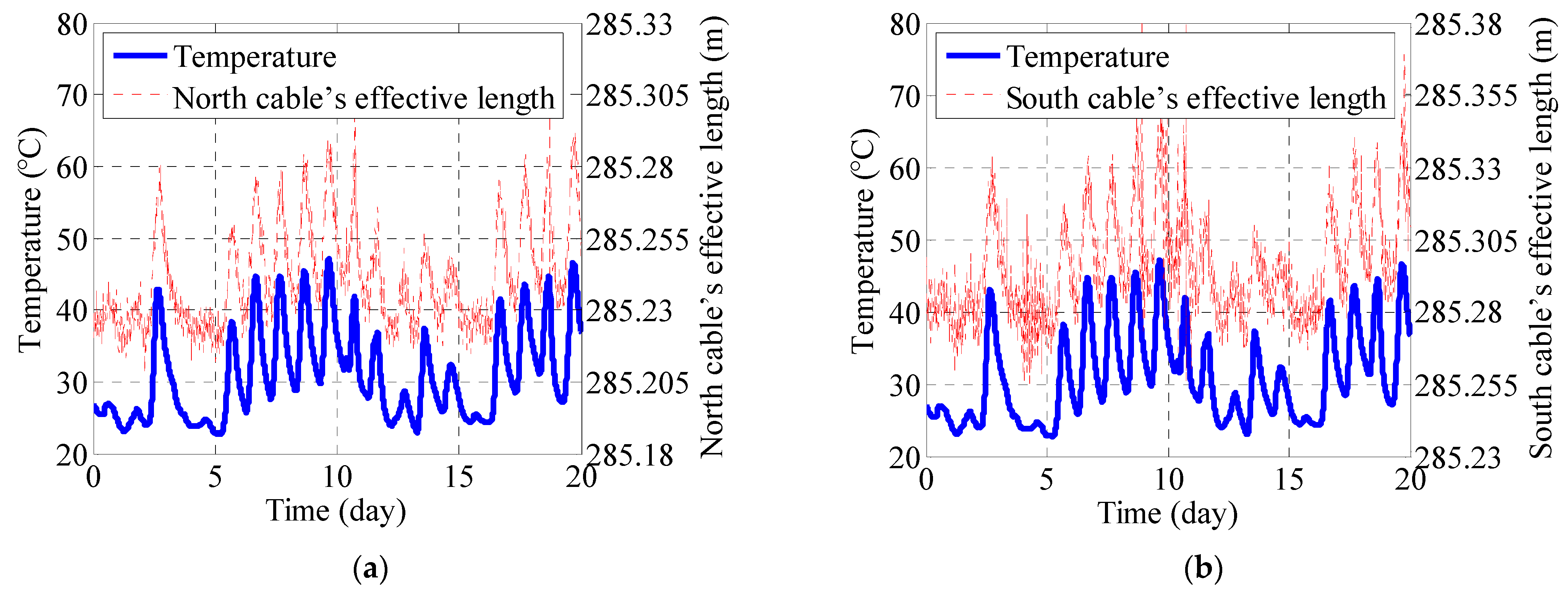
5.1. Calculation of Bridge Cable Length

In this paper, the tower-girder distance (effective cable length) is used instead of bridge cable length. Within material mechanics, the linear thermal expansion coefficient ($\alpha$) of a solid is defined as the fractional change in length per unit temperature change, relative to its original length, expressed as:

$$\alpha =\mathrm{\Delta }l/l_0\mathrm{\Delta }t$$

(5)

where $\alpha$ is the thermal expansion coefficient, and $l_0$ is the original length of the material. $\mathrm{\Delta }l$ and $\mathrm{\Delta }t$ are the length change and the temperature change, respectively. Similarly, the thermal expansion coefficient of bridge cables can be defined as:

$${\alpha }_e=\mathrm{\Delta }L/L_0\mathrm{\Delta }{T}_e$$

(6)

where ${\alpha }_e$ is the thermal expansion coefficient of the bridge cable. $L_0$ is the original length of the bridge cable. $\mathrm{\Delta }L$ and $\mathrm{\Delta }{T}_e$ are the length change and the temperature change of the bridge cable, respectively (Figure 16). Figure 16 shows the detailed positions of the North cable effective length and the South cable effective length.

Figure 17 indicates that the distance from the top of a bridge tower to the mid-span of the main beam effectively represents the length of the corresponding outermost cable. Correlation analysis and linear regression modeling were performed on the measured tower-beam distance (effective cable length) and temperature data collected between July 1st and 20th, 2014. Figure 17a,b show positive correlations between temperature and the effective lengths of the north and south cables, respectively, based on their correlation plots and fitted linear regression models.

As illustrated in Figure 1 (bridge structure diagram), the distance between each tower and the girder represents the length of the bridge’s outermost cable on that side. Consequently, this distance is used as a proxy for analyzing the outermost cable. This section examines the thermal expansion coefficients of the effective cable lengths—specifically, the north and south tower-girder distances—by correlating them with July 1st and 20th, 2014 temperature data and performing linear regression. The resultant linear regression analyses for the north and south effective cable lengths are shown in Figure 18a,b, respectively, with the corresponding regression equations displayed within each figure.

Table 4. The coefficient of thermal expansion for the cable’s effective length in the bridge structures.

Location	Sample Number	$\mathit{R}$	$\mathbf{\Delta }\mathit{L}/\mathbf{\Delta }{\mathit{T}}_{\mathbf{e}}$ $(\times {10}^{-4} \mathbf{m}/°\mathbf{C})$	${\mathit{L}}_0$ $\left(\mathbf{m}\right)$	Thermal Expansion Co-Efficient $(\times {10}^{-6}$ $/°\mathbf{C})$
North cable’s effective length	2880	0.96	34.93	285.11	12.25
South cable’s effective length	2880	0.89	34.04	285.11	11.94

details the thermal expansion coefficients of the bridge cables. Based on the structural diagram (Figure 1), the original cable length $L_0$ is 285.11 m. Using Equation (6), the coefficients $12.25\times {10}^{-6}/°\mathrm{C}$ and $11.94\times {10}^{-6}/°\mathrm{C}$ represent the thermal expansion coefficients for the effective lengths of the north and south cables, respectively, while $12\times {10}^{-6}/°\mathrm{C}$ is the coefficient for the strand cables. Consequently, this coefficient can function as a structural health indicator for bridge cables. Significant short-term deviations could signal structural damage, necessitating prompt inspection and maintenance.

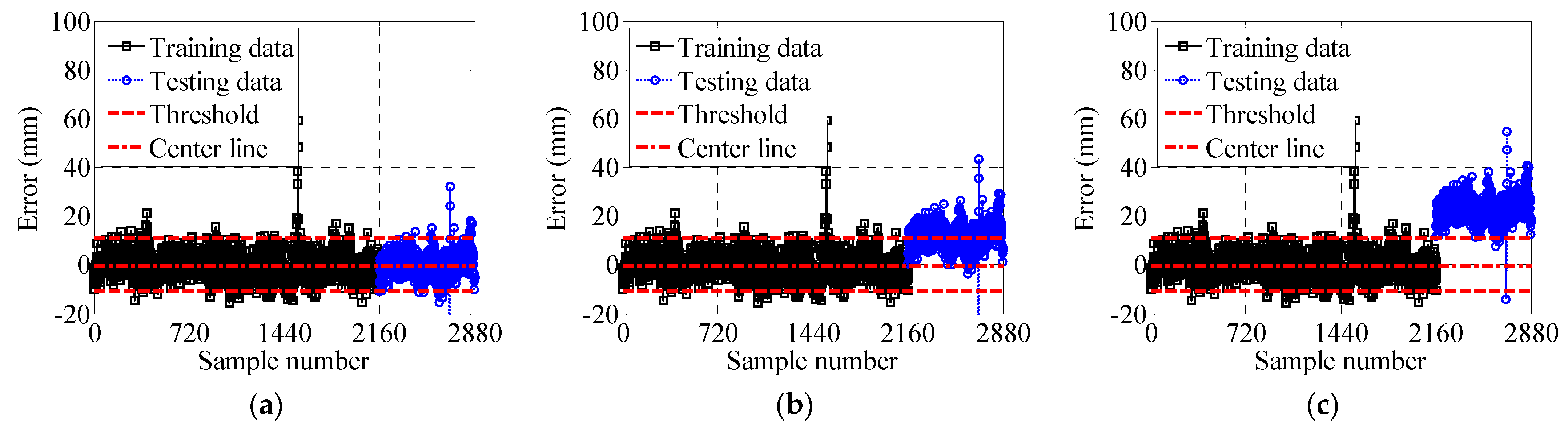
5.2. Bridge Cable Damage Warning Process

Bridges can be damaged when they are subjected to typhoons, vehicle overloading, hull impacts, corrosion and fatigue accidents, etc. Cracks or stiffness degradation in the bridge tower lead to an increase in its displacement response [32,33]. Wang et al. [34,35] used modeling residuals as a warning indicator for both the mid-span and towers. As a compression-bearing component, the bridge tower requires investigation of its mechanical characteristics, particularly compressive resistance, to ensure operational reliability [36,37]. The structural anomaly index is as follows:

$$e=L_m-L_e$$

(7)

where $e$ is the error in the effective cable length-temperature modeling. $L_m$ is the measured value of the effective cable length. $L_e$ is estimated value of the effective cable length.

The degradation expression is:

$$e_{de}=e+\epsilon L_0$$

(8)

where $e_{de}$ is the error in the displacement after damage. $e$ is the error in the effective cable length-temperature modeling. $\epsilon$ is the coefficient that adjusts the degree of the effective cable length damage, and $L_0$ is the original length of the effective cable length.

For the north cable, Case 1 represents the undamaged state, while Cases 2 to 6 correspond to increasing damage levels, from 0.5% to 2.5%. Similarly, for the south cable, Case 7 is the undamaged state, and Cases 8 to 12 represent damage, increasing from 0.5% to 2.5%. In July 2014, a study investigated effective cable length error performance warnings using 4464 data point samples. The first 15 days served as training data, and the subsequent 5 days as testing data. The impact of significance levels ($\omega$ = 0.05, 0.01, 0.003) on warning performance was analyzed. $\omega$ = 0.05 is the most widely accepted and used standard in fields such as social sciences, life sciences, and psychology, and a= 0.01 is in medical research (especially when it comes to high-risk treatments or drug approvals). According to the “Technical Standard for Building Structure Inspection” of China, $\omega$ = 0.05 is the basic setting. Huang et al. [38] proposed a long-term monitoring performance early warning method for bridge main beams based on strain, in which the significance levels were set at 0.05, 0.01, and 0.003. Wang et al. [39] proposed a bridge performance early warning method based on multi-order frequencies and studied the influence of the significance level and the consideration of modal order on the early warning rate. In this paper, $\omega$ = 0.05 was set as the basis and standard value for early warning research. Its threshold is the widest, and it is the most difficult threshold to trigger for an early warning. $\omega$ = 0.01 is taken as the threshold for an easier early warning to start. The threshold width of $\omega$ = 0.003 is the narrowest and the most likely to trigger the early warning.

As the significance level rises,

Table 5. North cable warning rates.

Case Number	$\mathit{\omega }$ = 0.05		$\mathit{\omega }$ = 0.01		$\mathit{\omega }$ = 0.003
	Alam Number	Alam Rate (%)	Alam Number	Alam Rate (%)	Alam Number	Alam Rate (%)
Case 1	20	2.78	8	1.11	5	0.69
Case 2	402	55.83	223	30.97	107	14.86
Case 3	717	99.58	682	94.72	643	89.31
Case 4	719	99.86	719	99.86	719	99.86
Case 5	719	99.86	719	99.86	719	99.86
Case 6	720	100	720	100	720	100

and

Table 6. South cable warning rates.

Case Number	$\mathit{\omega }$ = 0.05		$\mathit{\omega }$ = 0.01		$\mathit{\omega }$ = 0.003
	Alam Number	Alam Rate (%)	Alam Number	Alam Rate (%)	Alam Number	Alam Rate (%)
Case 7	7	0.97	4	0.56	2	0.28
Case 8	71	9.86	17	2.36	7	0.97
Case 9	358	49.72	141	19.58	69	9.58
Case 10	684	95	504	70	347	48.19
Case 11	720	100	714	99.17	677	94.03
Case 12	720	100	720	100	720	100

show increasing warning counts and rates for performance degradation in the north and south effective cable lengths, respectively. Notably, Table 5 shows that the north cable (Case 6) achieved a 100% warning rate for damage exceeding 2.5%, while Table 6 indicates the south cable (Case 11) detected deformation as low as 2.0% with a 100% warning rate.

Figure 19 and Figure 20 display performance warnings for the north and south effective cable lengths, utilizing thresholds established from training data. Specifically, Figure 19a identifies Case 1 as the normal operating state for the north cable. Figure 19b–f reveal an increasing number of north cable samples exceeding the control threshold. A similar trend appears for the south cable in Figure 20b–f. As Figure 19f and Figure 20e illustrate, all test data points in Case 6 and Case 11 surpass the threshold, triggering warnings for 100% of samples.

6. Conclusions

This paper, through the analysis of monitoring data, reveals the correlation between temperature and the displacement of bridge towers, the length of cables, etc. Correlation modeling was conducted on the corrected monitoring data, and the early warning method for bridge cables was formulated using the modeling residuals. The conclusions are as follows.

The skipping abnormal repair method based on the three-sigma rule, the missing abnormal repair method of multiple linear regression and interpolation method, and the constant abnormal repair method of $\mathrm{NaN}$ calibration were proposed. The proposed methods effectively repaired the air temperature, structural temperature, and displacement monitoring data.

The variation trends in air temperature and structural temperature are the same, and the peak value of the structural temperature is significantly higher than that of the air temperature. The air temperature sensor is closer to the north-south cables and exposed to the air. The structural temperature sensor is installed inside the main beam steel box girder, so the air temperature can better represent the temperature of the cables.

The north tower displacement exhibits a strong positive correlation with the air temperature (correlation coefficient = 0.87), and the south tower displacement is also strongly positively correlated with the air temperature (correlation coefficient = 0.91). The north cable’s effective length and the south cable’s effective length are both highly positively correlated with the air temperature (the correlation coefficients are 0.94 and 0.93, respectively).

The monitoring data from July 1st to 20th were selected for early warning research. The fitting equation was calculated through the effective cable length, and then the thermal expansion coefficient $12.25\times {10}^{-6}/°\mathrm{C}$ (north) and $11.94\times {10}^{-6}/°\mathrm{C}$ (south) were further calculated. These values match the design coefficient $12\times {10}^{-6}/°\mathrm{C}$.

An effective cable length error was introduced as a performance warning indicator. Using control charts on six damage cases, the method achieved 100% warning rates for both the north cable (Case 6) and south cable (Case 11). This approach successfully detected reductions of 2.5% and 2.0% for the north and south cables, respectively.

References

1. Li, D.L.; Yang, D.H.; Yi, T.H.; Zhang, S.H. Anomaly diagnosis of stay cables based on vehicle-induced cable force sums. Eng. Struct. 2023, 289, 116239. [Google Scholar] [CrossRef]
2. Zheng, X.W.; Hou, Y.Z.; Cheng, J.; Xu, S.; Wang, W.M. Rapid Damage Assessment and Bayesian-Based Debris Prediction for Building Clusters Against Earthquakes. Buildings 2025, 15, 1481. [Google Scholar] [CrossRef]
3. Zheng, X.W.; Lv, H.L.; Fan, H.; Zhou, Y.B. Physics-Based Shear-Strength Degradation Model of Stud Connector with the Fatigue Cumulative Damage. Buildings 2022, 12, 2141. [Google Scholar] [CrossRef]
4. Zheng, X.W.; Li, H.N.; Gardoni, P. Hybrid Bayesian-Copula-based risk assessment for tall buildings subject to wind loads considering various uncertainties. Reliab. Eng. Syst. Safe. 2023, 233, 109100. [Google Scholar] [CrossRef]
5. Zacchei, E.; Lyra, P.H.C.; Lage, G.E.; Antonine, E.; Soares, A.B., Jr.; Caruso, N.C.; De Assis, C.S. Structural Health Monitoring of a Brazilian Concrete Bridge for Estimating Specific Dynamic Responses. Buildings 2022, 12, 785. [Google Scholar] [CrossRef]
6. Radulescu, V.M.; Radulescu, G.M.T.; Nas, S.M.; Radulescu, A.T.; Radulescu, C.M. Structural Health Monitoring of Bridges under the Influence of Natural Environmental Factors and Geomatic Technologies: A Literature Review and Bibliometric Analysis. Buildings 2024, 14, 2811. [Google Scholar] [CrossRef]
7. Rabi, R.R.; Vailati, M.; Monti, G. Effectiveness of Vibration-Based Techniques for Damage Localization and Lifetime Prediction in Structural Health Monitoring of Bridges: A Comprehensive Review. Buildings 2024, 14, 1183. [Google Scholar] [CrossRef]
8. Pei, X.Y.; Hou, Y.; Huang, H.B.; Zheng, J.X. A Multi-Objective Sensor Placement Method Considering Modal Identification Uncertainty and Damage Detection Sensitivity. Buildings 2025, 15, 821. [Google Scholar] [CrossRef]
9. Zheng, X.W.; Li, H.N.; Gardoni, P. Reliability-based design approach for high-rise buildings subject to earthquakes and strong winds. Buildings 2021, 244, 112771. [Google Scholar] [CrossRef]
10. Di Trapani, F.; Oddo, M.C.; Sberna, A.P.; La Mendola, L. Structural health monitoring of masonry structures using stress sensors: Experimental induced damage tests and proposed approach for real-time monitoring. Constr. Build. Mater. 2024, 449, 138077. [Google Scholar] [CrossRef]
11. Tao, T.Y.; Wang, H.; Wen, X.H.; Fenerci, A. Flutter analysis of a long-span triple-tower suspension bridge under typhoon winds with non-uniform spanwise profile. Structures 2024, 68, 107156. [Google Scholar] [CrossRef]
12. Saad, S.; Nasir, A.; Bashir, R.; Pantazopoulou, S.J. Numerical Study on the Effect of Climate Parameters on the Extreme Thermal Gradients in Concrete Box Girders. J. Bridge Eng. 2023, 28, 04023069. [Google Scholar] [CrossRef]
13. Marco, D.; Raffaele, C. Structural Resilience through Structural Health Monitoring. In Data Driven Methods for Civil Structural Health Monitoring and Resilience, 1st ed.; Parsa, G., Seyed, S.K., Andy, N., Eds.; CRC Press: Boca Raton, FL, USA, 2023; Volume 1, pp. 1–13. [Google Scholar] [CrossRef]
14. Zhang, L.X.; Qiu, G.Y.; Chen, Z.S. Structural health monitoring methods of cables in cable-stayed bridge: A review. Measurement 2020, 168, 108343. [Google Scholar] [CrossRef]
15. Jin, S.S.; Jeong, S.; Sim, S.H.; Seo, D.W.; Park, Y.S. Fully automated peak-picking method for an autonomous stay-cable monitoring system in cable-stayed bridges. Automat. Constr. 2021, 126, 103628. [Google Scholar] [CrossRef]
16. Wang, L.S.; Zhao, C.; Lan, C.G. Stay cable tension estimation using a vision-based monitoring system under complex environments. Meas. Sci. Technol. 2021, 36, 026009. [Google Scholar] [CrossRef]
17. Lin, J.H.; Briseghella, B.; Xue, J.Q.; Tabatabai, H. Temperature Monitoring and Response of Deck-Extension Side-by-Side Box Girder Bridges. J. Perform. Constr. Fac. 2020, 34, 04019122. [Google Scholar] [CrossRef]
18. Zhu, Q.X.; Wang, H.; Spencer, B.F. Investigation on the mapping for temperature-induced responses of a long-span steel truss arch bridge. Struct. Infrastruct. Eng. 2024, 20, 232–249. [Google Scholar] [CrossRef]
19. Xu, S.Y.; Wang, G.X.; Zhu, J.; Chen, B. Probabilistic statistical evaluation of the design values of temperature differences of steel truss girder bridges through finite element simulation and monitoring data analysis. J. Civ. Struct. Health 2025, 15, 1403–1420. [Google Scholar] [CrossRef]
20. Xia, Q.; Wu, W.L.; Li, F.N.; Zhou, X.Q. Temperature behaviors of an arch bridge through integration of field monitoring and unified numerical simulation. Adv. Struct. Eng. 2022, 25, 3492–3509. [Google Scholar] [CrossRef]
21. Elshoura, A.; Okeil, A.M. Simplified method for estimating restraint moment induced by vertical temperature gradient in continuous prestressed concrete bridges and verification using AASHTO BDS. Struct. Infrastruct. Eng. 2024, 20, 944–956. [Google Scholar] [CrossRef]
22. Wang, G.X.; Shao, J.S.; Xu, W.Z.; Dong, Z.X. Real-time quantitative evaluation on the cable damage of cable-stayed bridges using the correlation between girder deflection and temperature. Struct. Health Monit. 2022, 21, 1483–1500. [Google Scholar] [CrossRef]
23. Fu, C.Y.; Liu, Y.P.; Lao, Y.S. Assessing Temperature-Induced Deflections in Cable-Stayed Bridges during Construction: An Elastic Foundation Beam Model Approach. J. Bridge Eng. 2025, 30, 04024104. [Google Scholar] [CrossRef]
24. Zhu, Q.X.; Wang, H.; Mao, J.X.; Wan, H.P. Investigation of Temperature Effects on Steel-Truss Bridge Based on Long-Term Monitoring Data: Case Study. J. Bridge Eng. 2020, 25, 05020007. [Google Scholar] [CrossRef]
25. Gong, X.Y.; Song, X.D.; Cai, C.S.; Li, G.Q. Early warning for abnormal strains of continuous bridges using a proposed temperature-strain mapping model. Smart Mater. Struct. 2023, 32, 125018. [Google Scholar] [CrossRef]
26. Zhu, Y.; Sun, D.Q.; Guo, H.; Shuang, M. Fine analysis for non-uniform temperature field and effect of railway truss suspension bridge under solar radiation. J. Constr. Steel Res. 2023, 210, 108098. [Google Scholar] [CrossRef]
27. Li, J.X.; Yi, T.H.; Qu, C.X.; Li, H.N. Early Warning for Abnormal Cable Forces of Cable-Stayed Bridges Considering Structural Temperature Changes. J. Bridge Eng. 2023, 28, 04022137. [Google Scholar] [CrossRef]
28. Yang, D.H.; Gu, H.L.; Yi, T.H.; Li, H.N. Bridge Cable Anomaly Detection Based on Local Variability in Feature Vector of Monitoring Group Cable Forces. J. Bridge Eng. 2023, 28, 04023030. [Google Scholar] [CrossRef]
29. Chen, Q.; Wang, H.F.; El-Tawil, S.; Agrawal, A.K. Progressive Collapse Behavior of a Long-Span Cable-Stayed Bridge Induced by Cable Loss. J. Bridge Eng. 2023, 28, 05023005. [Google Scholar] [CrossRef]
30. Kong, X.; Liu, Z.W.; Liu, H.; Hu, J.X. Recent advances on inspection, monitoring, and assessment of bridge cables. Automat. Constr. 2024, 168, 105767. [Google Scholar] [CrossRef]
31. Huang, H.B.; Yi, T.H.; Li, H.N.; Liu, H. Sparse Bayesian Identification of Temperature-Displacement Model for Performance Assessment and Early Warning of Bridge Bearings. J. Struct. Eng. 2022, 148, 04022052. [Google Scholar] [CrossRef]
32. Yang, T.Y.; Liu, K.; Nie, G.B. Improved Time Domain Substructural Damage Identification Method on Large-Span Spatial Structure. Shock Vib. 2021, 2021, 1069470. [Google Scholar] [CrossRef]
33. Nie, G.B.; Yang, T.Y.; Zhi, X.D.; Liu, K. Damage evaluation of square steel tubes at material and component levels based on a cyclic loading experiment. Adv. Mech. Eng. 2018, 10, 1687814018797786. [Google Scholar] [CrossRef]
34. Wang, Y.; Yang, D.H.; Yi, T.H. Displacement model error-based method for symmetrical cable-stayed bridge performance warning after eliminating variable load effects. J. Civ. Struct. Health 2022, 12, 81–99. [Google Scholar] [CrossRef]
35. Wang, Y.; Yang, D.H.; Yi, T.H. Accurate Correlation Modeling between Wind Speed and Bridge Girder Displacement Based on a Multi-Rate Fusion Method. Sensors 2021, 21, 1967. [Google Scholar] [CrossRef] [PubMed]
36. Wang, W.N.; Gong, J.X. New relaxation function and age-adjusted effective modulus expressions for creep analysis of concrete structures. Eng. Struct. 2019, 188, 1–10. [Google Scholar] [CrossRef]
37. Wang, W.N.; Gong, J.X.; Wu, X.Y.; Wang, X.C. A general equation for estimation of time-dependent prestress losses in prestressed concrete members. Structures 2023, 55, 278–293. [Google Scholar] [CrossRef]
38. Huang, H.B.; Yi, T.H.; Li, H.N.; Liu, H. Strain-Based Performance Warning Method for Bridge Main Girders under Variable Operating Conditions. J. Bridge Eng. 2020, 25, 04020013. [Google Scholar] [CrossRef]
39. Wang, Z.; Yi, T.H.; Li, H.N.; Liu, H. Multiorder Frequency-Based Integral Performance Warning of Bridges Considering Multiple Environmental Effects. J. Struct. Eng. 2023, 28, 04022230. [Google Scholar] [CrossRef]
Figure 1. Bridge elevation and sensor positioning (unit: m).
Buildings 15 02342 g001
Figure 2. Rectify the skipped abnormal air temperature monitoring data using the three-sigma rule method: (a) original air temperature data and (b) data repaired via the three-sigma rule method.
Buildings 15 02342 g002
Figure 3. Utilize multiple linear regression to restore the missing abnormal structural temperature monitoring data for the periods: (a) 5–15 January 2014 and (b) 16–26 January 2014.
Buildings 15 02342 g003
Figure 4. Use interpolation to repair missing abnormal mid-span displacement monitoring data: (a) longitudinal displacement and (b) vertical displacement.
Buildings 15 02342 g004
Figure 5. Correction of constant displacement monitoring data: (a) displacement time-history curve before calibration and (b) displacement time-history curve after NaN calibration.
Buildings 15 02342 g005
Figure 6. Variation tendency in the air temperature in 2014: (a) WSD-1-01; (b) WSD-2-01; (c) WSD-2-02; and (d) WSD-3-01.
Buildings 15 02342 g006
Figure 7. The time-history curves of the air temperature: (a) July 2014 and (b) 22–23 July 2014.
Buildings 15 02342 g007
Figure 8. The variation tendency of the structure temperature in 2014: (a) NO7; (b) NA6; (c) north tower; (d) NJ8; (e) mid-span; (f) SJ8; (g) south tower; (h) SA6; and (i) SO7.
Buildings 15 02342 g008
Figure 9. The average structure temperature distribution of the whole bridge in July 2014.
Buildings 15 02342 g009
Figure 10. Air and structural temperature variations.
Buildings 15 02342 g010
Figure 11. Displacement over time for the north and south towers during June and July 2014.
Buildings 15 02342 g011
Figure 12. Comparing temporal variability of air temperature and tower displacement (9–12 July): (a) north tower and (b) south tower.
Buildings 15 02342 g012
Figure 13. Linear regression between air temperature and tower displacement: (a) north tower and (b) south tower.
Buildings 15 02342 g013
Figure 14. Comparing temporal variability of air temperature and tower-girder distance (9–12 July): (a) north tower-girder distance and (b) south tower-girder distance.
Buildings 15 02342 g014
Figure 15. Linear regression between air temperature and tower-girder distance: (a) north tower-girder distance and (b) south tower-girder distance.
Buildings 15 02342 g015
Figure 16. Schematic diagram of outermost cable lengths of bridge.
Buildings 15 02342 g016
Figure 17. Comparison between the time variabilities of the air temperature and effective cable length in July 2014: (a) North cable’s effective length and (b) South cable’s effective length.
Buildings 15 02342 g017
Figure 18. Linear regression analysis of the relationship between the air temperature and effective cable length (July 2014): (a) North cable’s effective length and (b) South cable’s effective length.
Buildings 15 02342 g018
Figure 19. North cable warning control chart: (a) Case 1; (b) Case 2; (c) Case 3; (d) Case 4; (e) Case 5; and (f) Case 6.
Buildings 15 02342 g019aBuildings 15 02342 g019b
Figure 20. South cable warning control chart: (a) Case 7; (b) Case 8; (c) Case 9; (d) Case 10; (e) Case 11; and (f) Case 12.
Buildings 15 02342 g020