
Time-Dependent Fragility Functions and Post-Earthquake Residual Seismic Performance for Existing Steel Frame Columns in Offshore Atmospheric Environment

Abstract
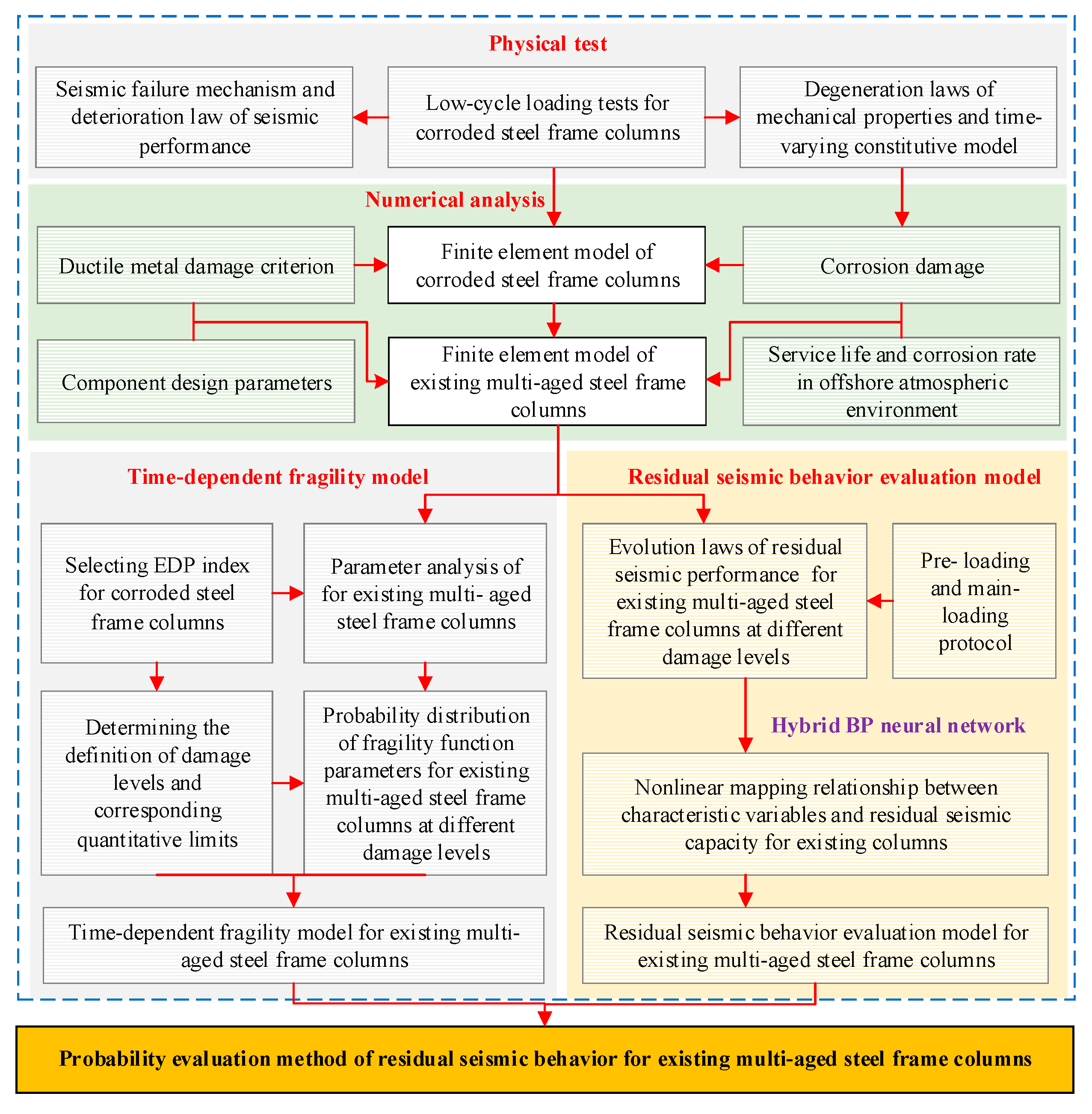
1. Introduction
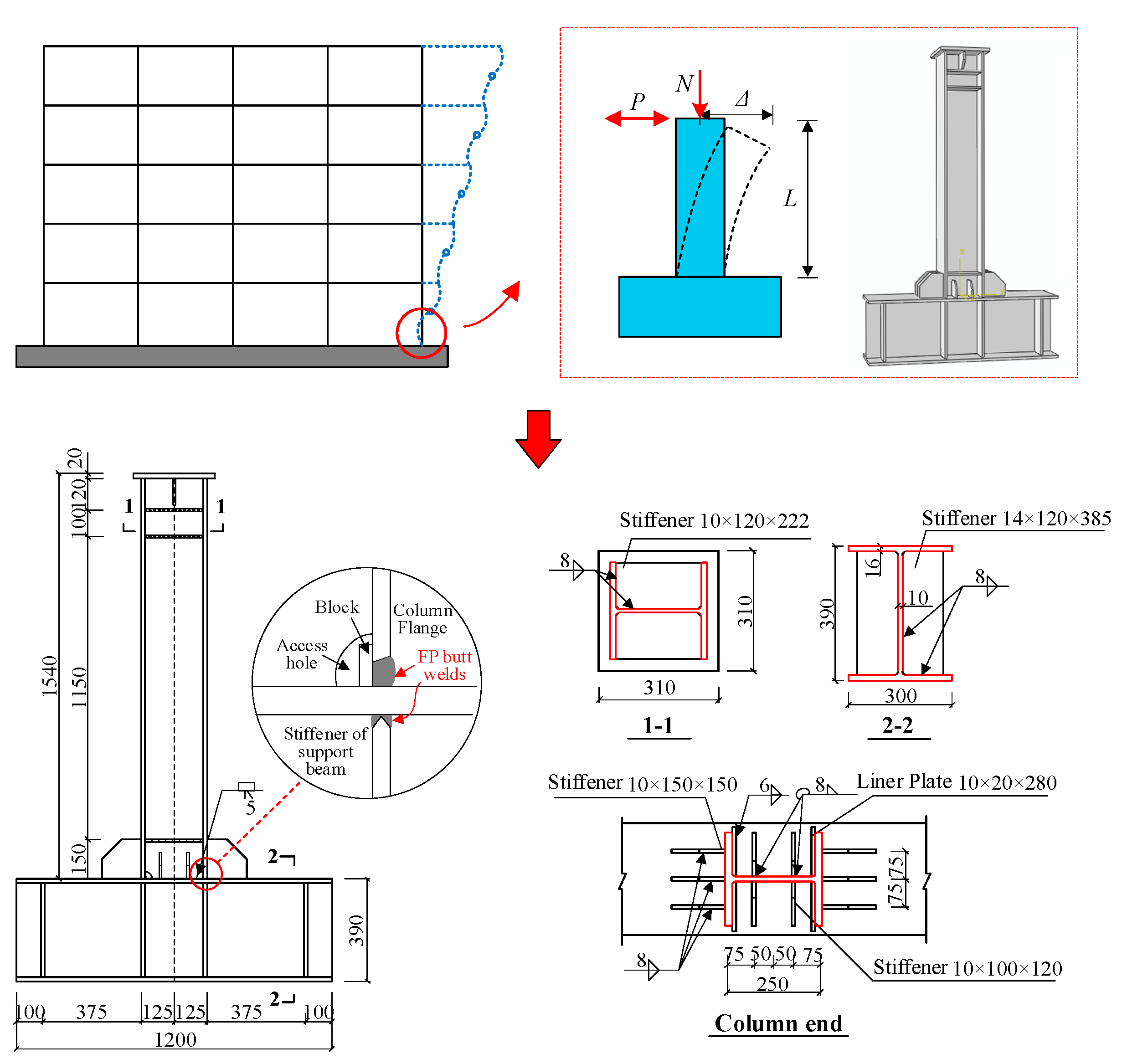
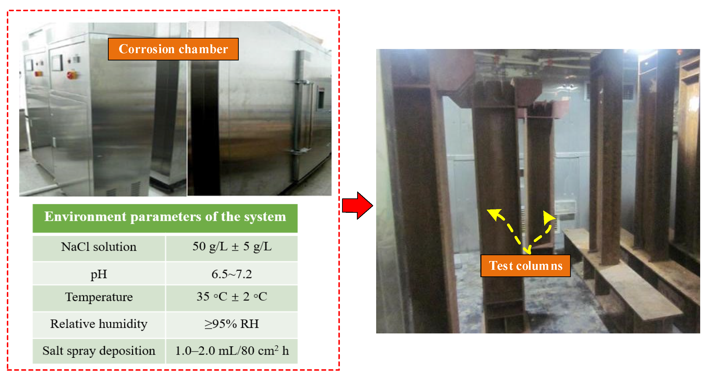
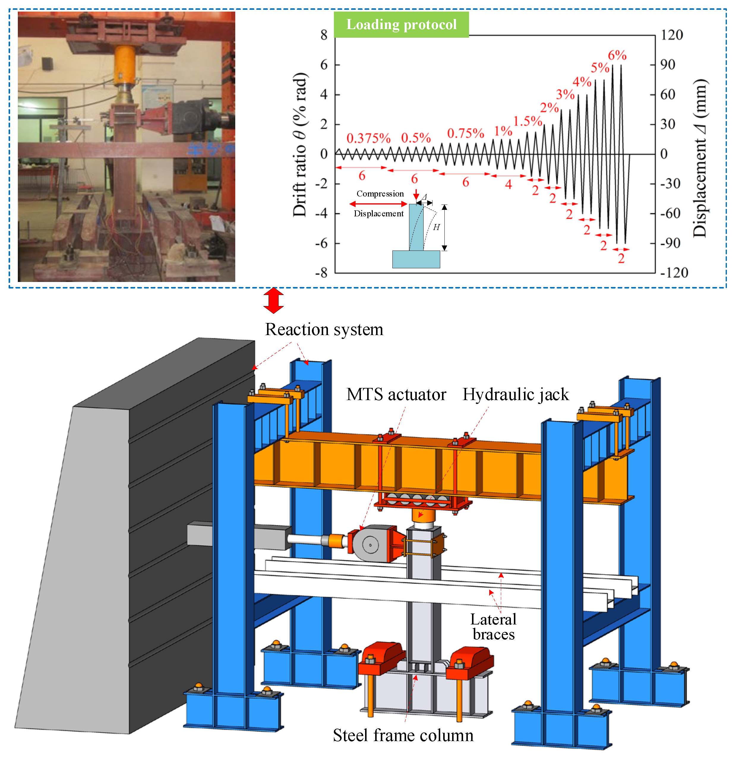
2. Low-Cycle Loading Tests
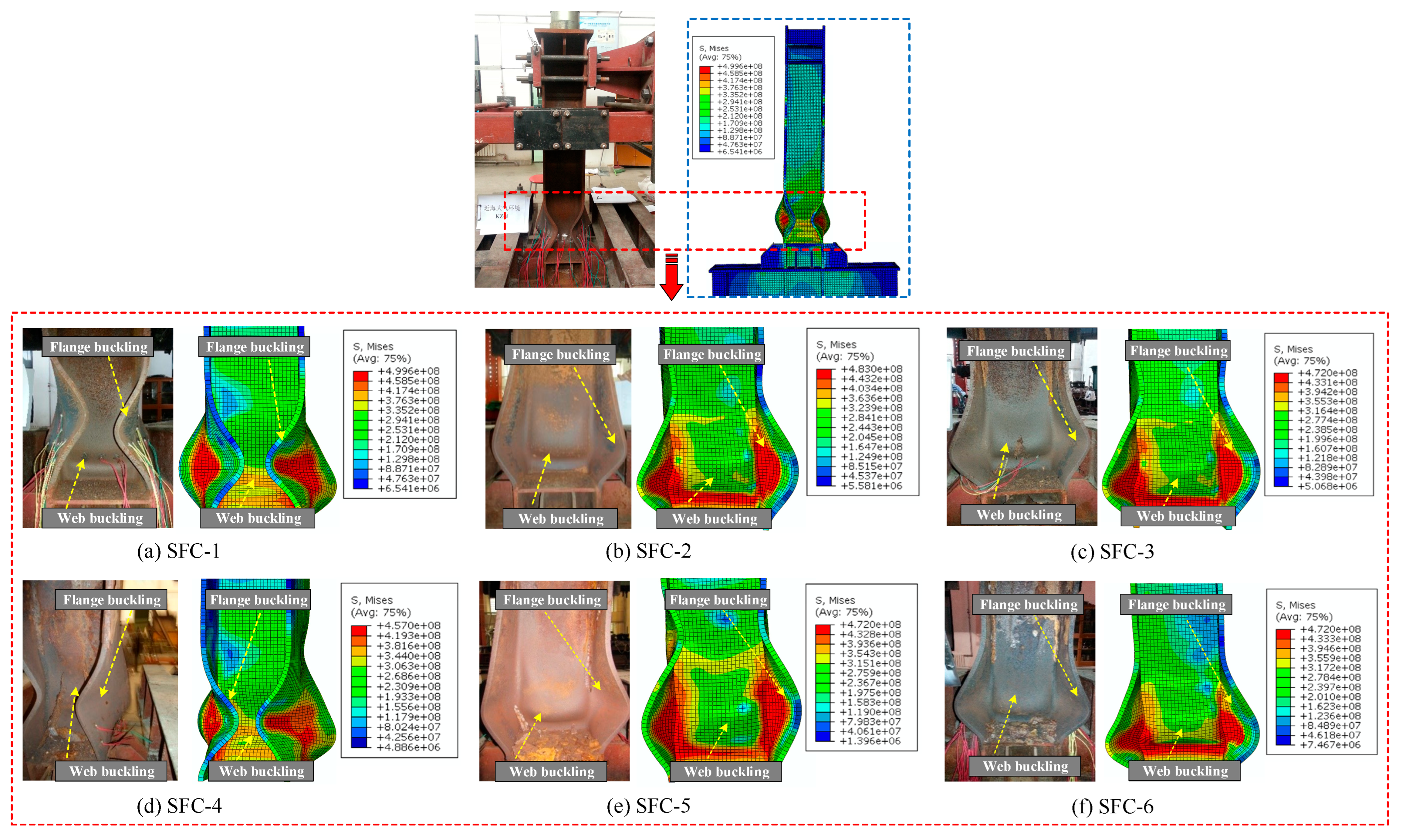
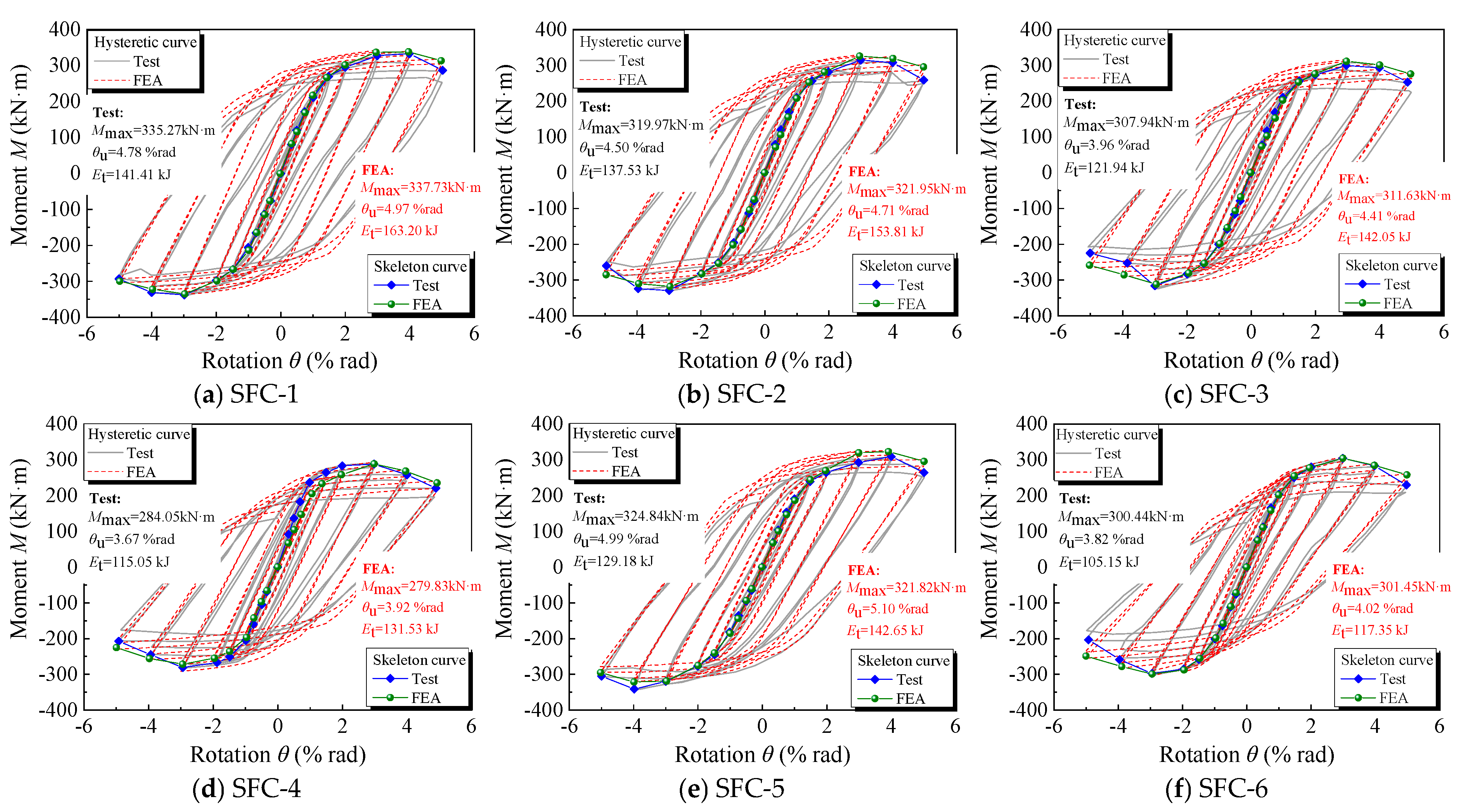
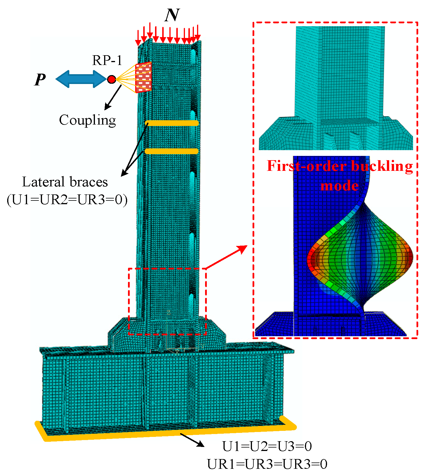
3. Finite Element Analysis
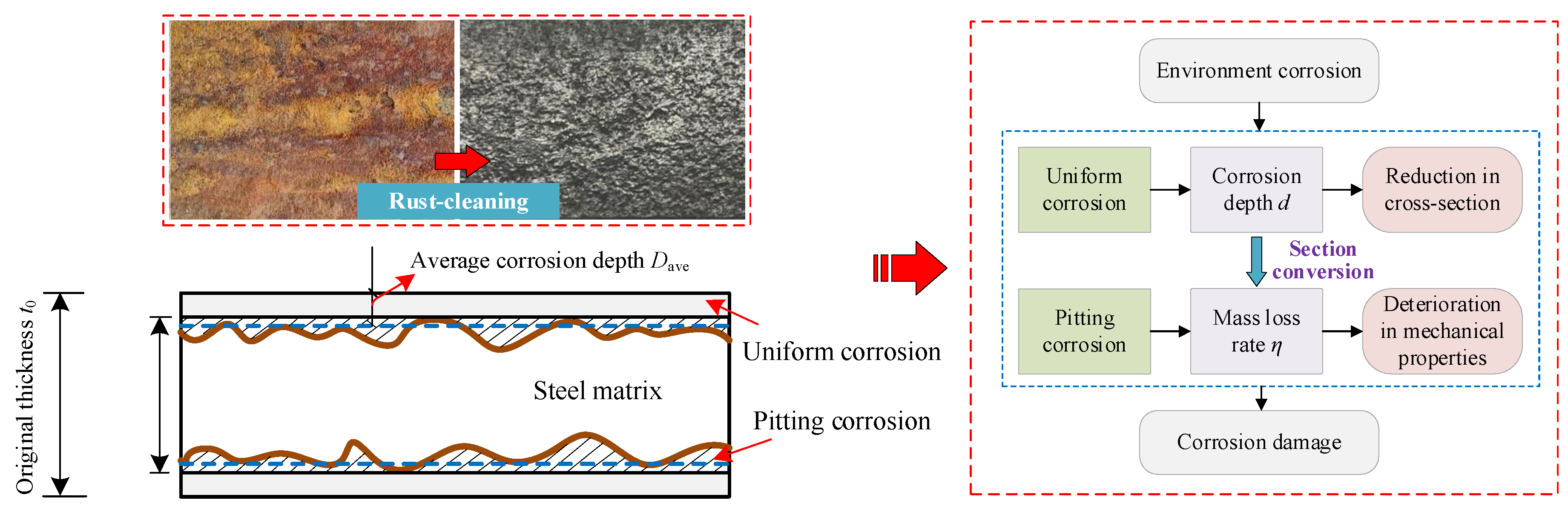
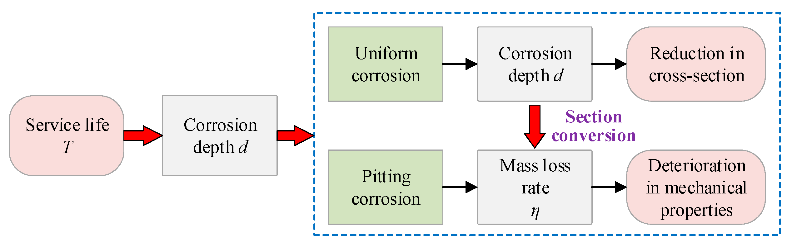
- (1)
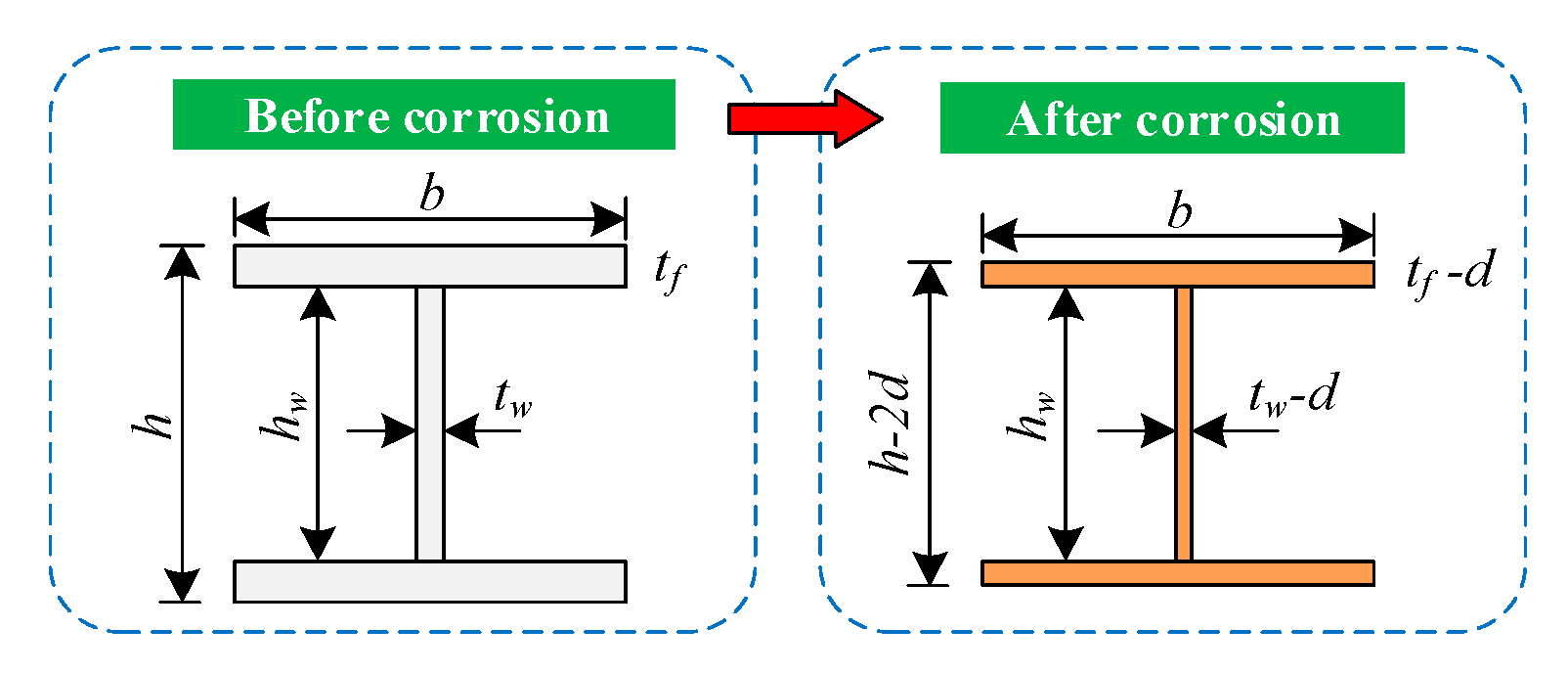
- Uniform corrosion was characterized by a reduction in the cross-sectional size of the column.
- (2)
- Pitting corrosion was characterized by the degeneration laws of the mechanical properties of steel with an increasing mass loss rate η, as shown in Equation (3), as discussed in the author’s previous research [31]. The maximum residual thickness was used to determine the mechanical properties.
4. Time-Dependent Fragility Analysis
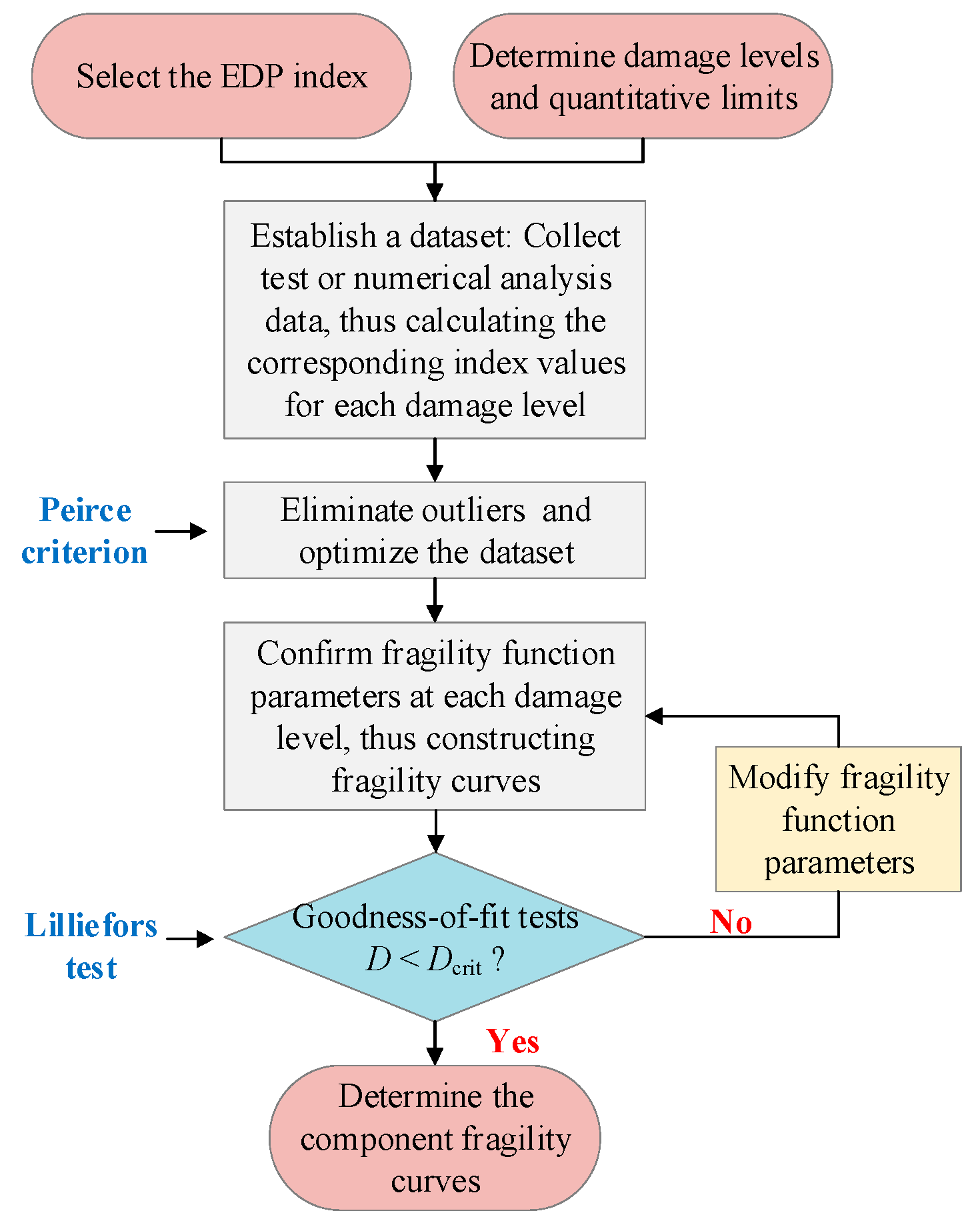
4.1. Fragility Function
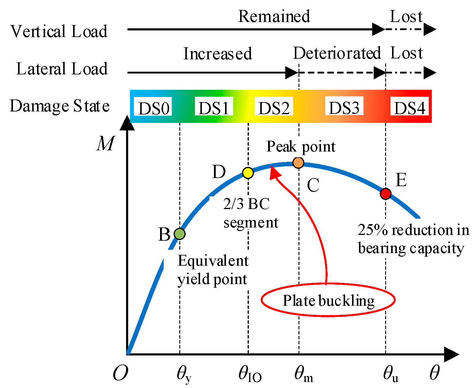
4.2. Classification Criteria of Damage States
4.3. Dataset for Fragility Function Parameters
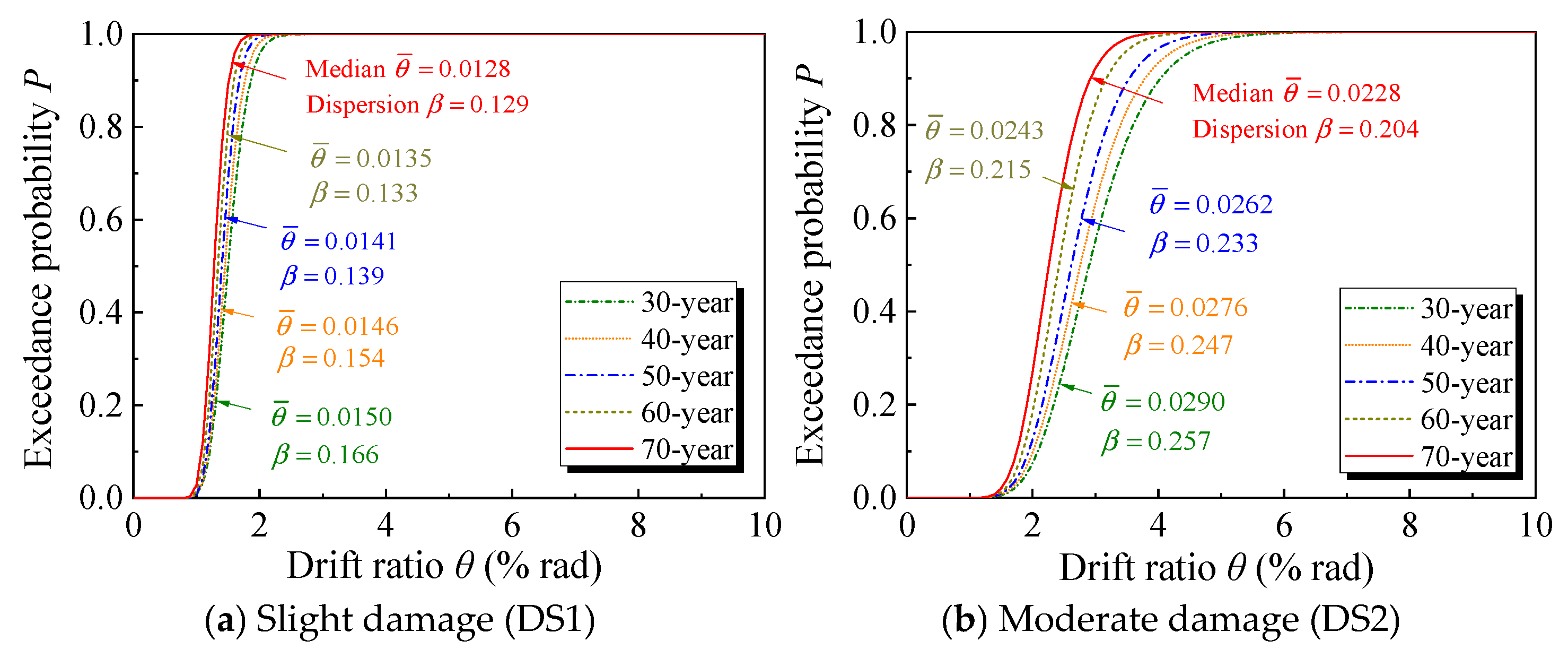
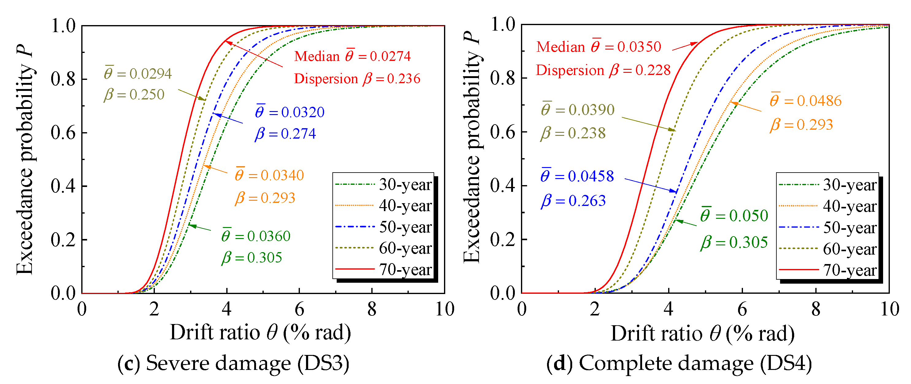
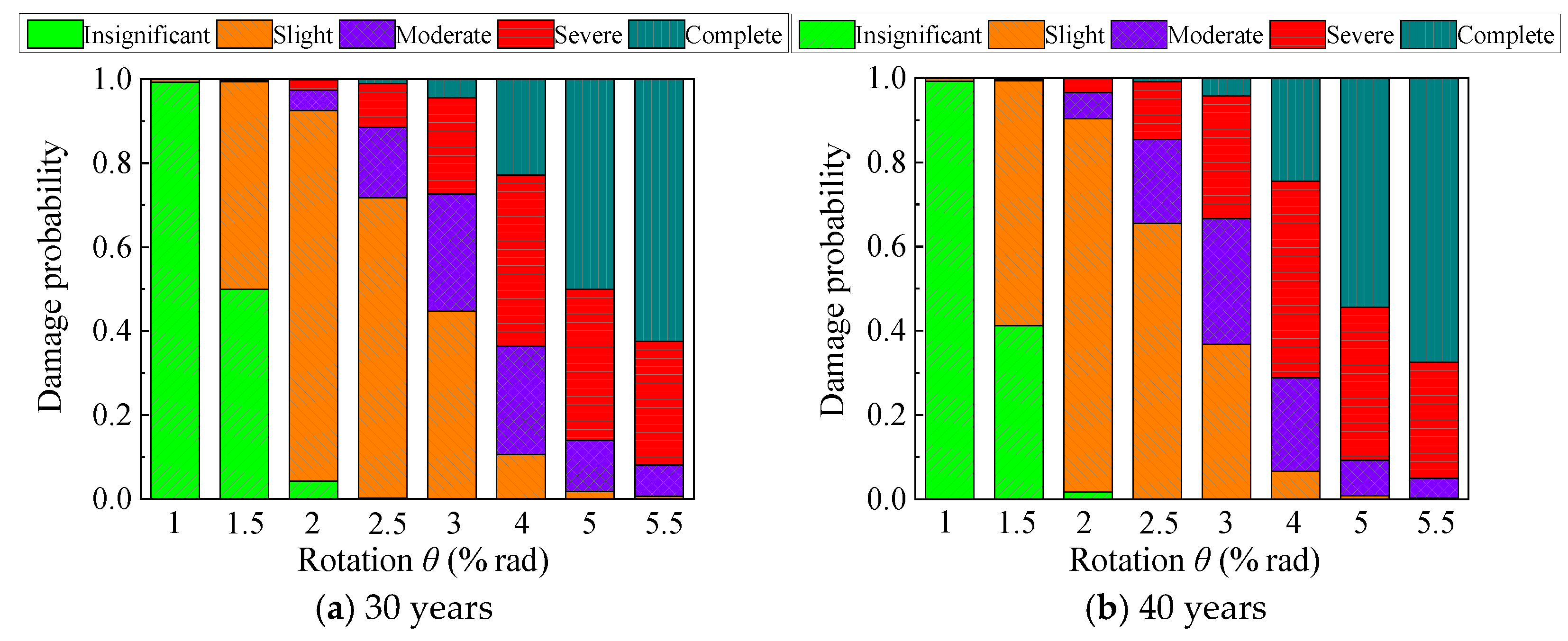
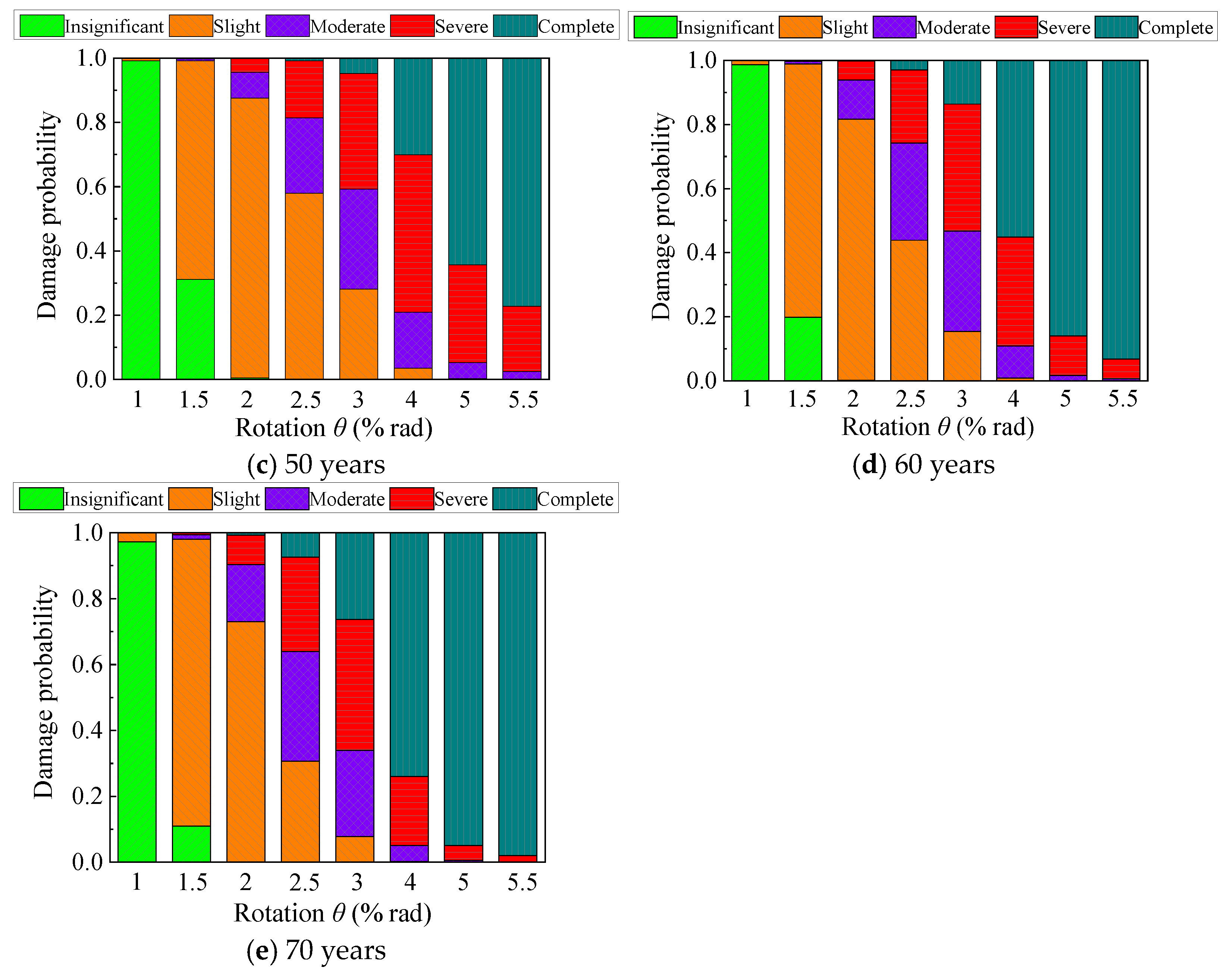
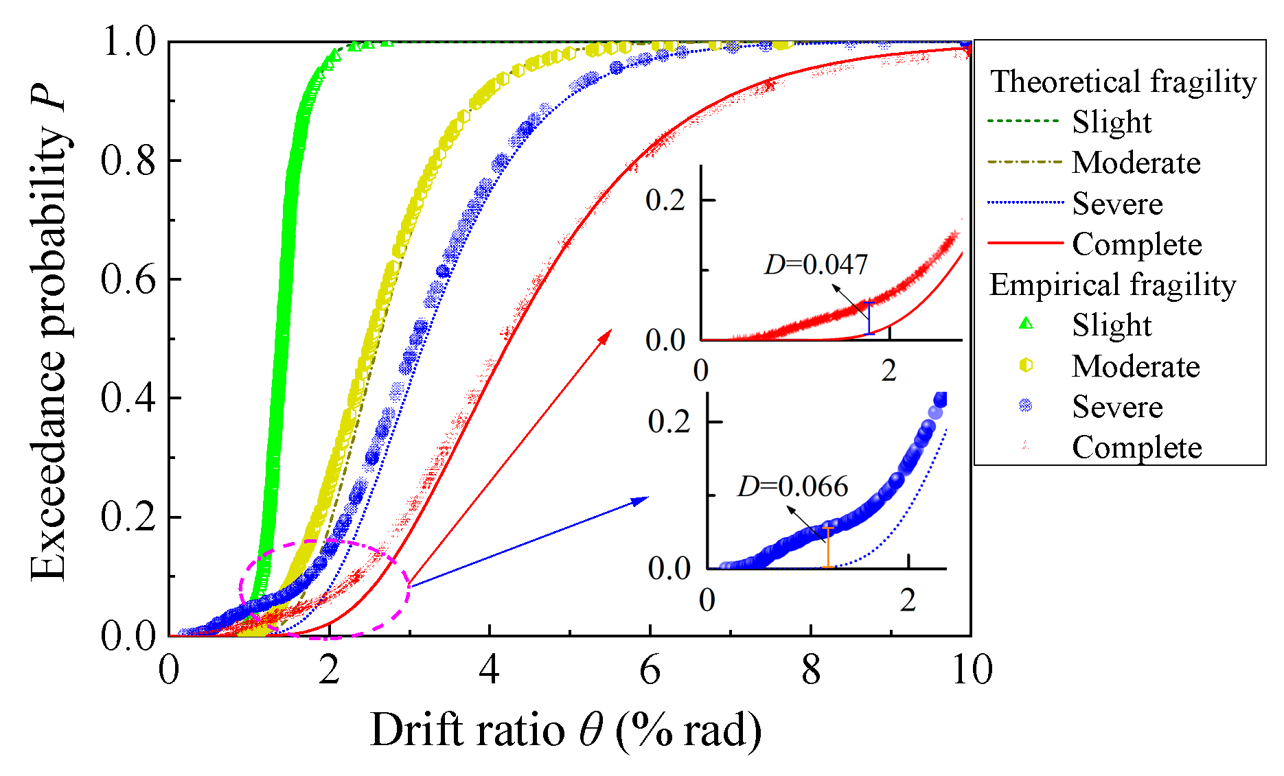
4.4. Fragility Analysis
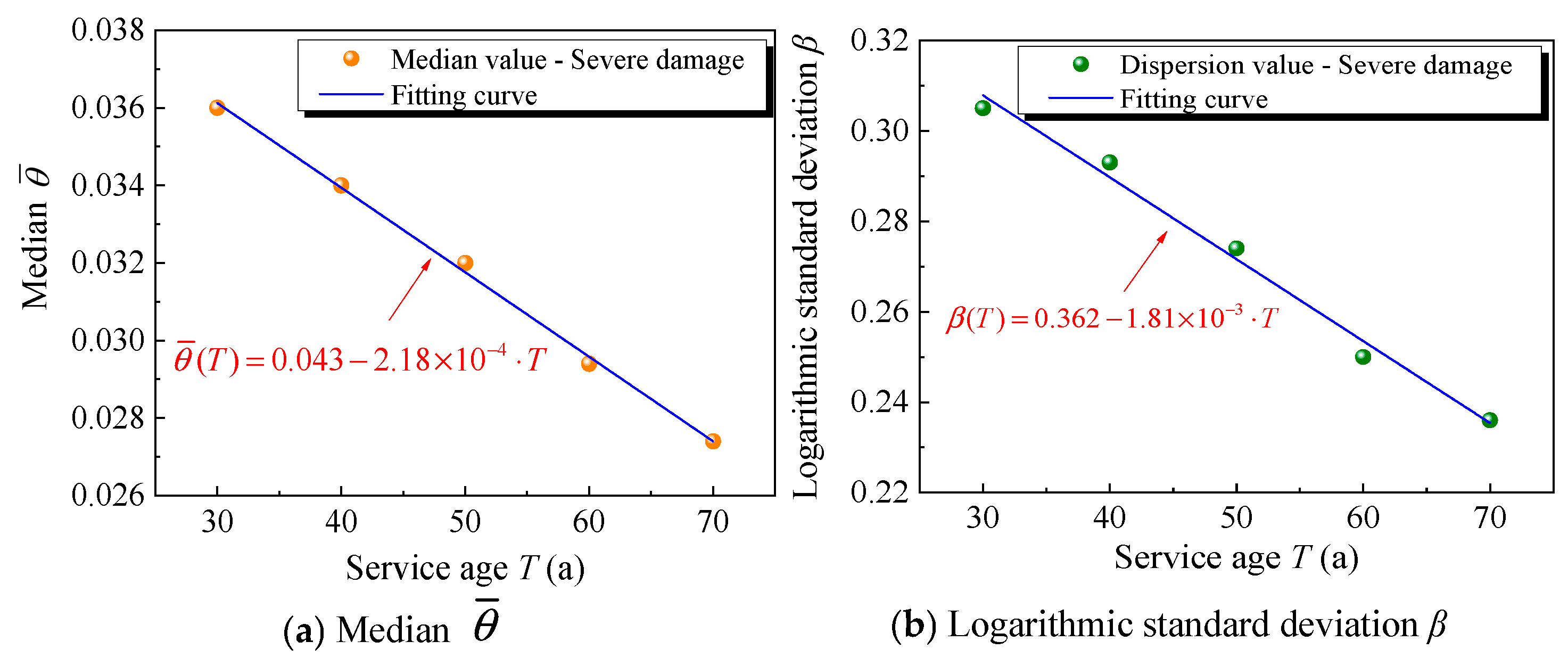
4.5. Time-Dependent Fragility Model
5. Residual Seismic Behavior Evaluation
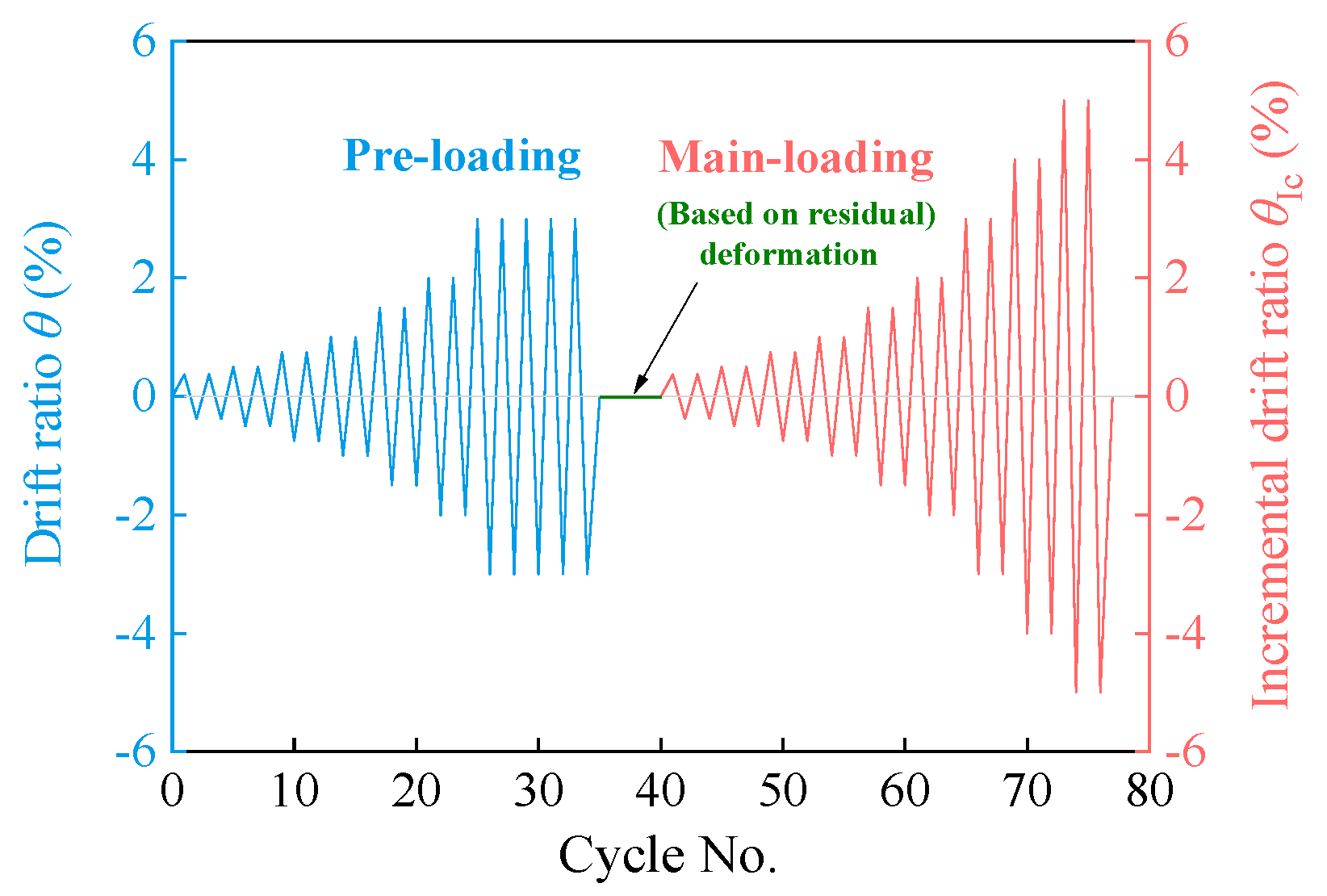
5.1. Loading Scheme
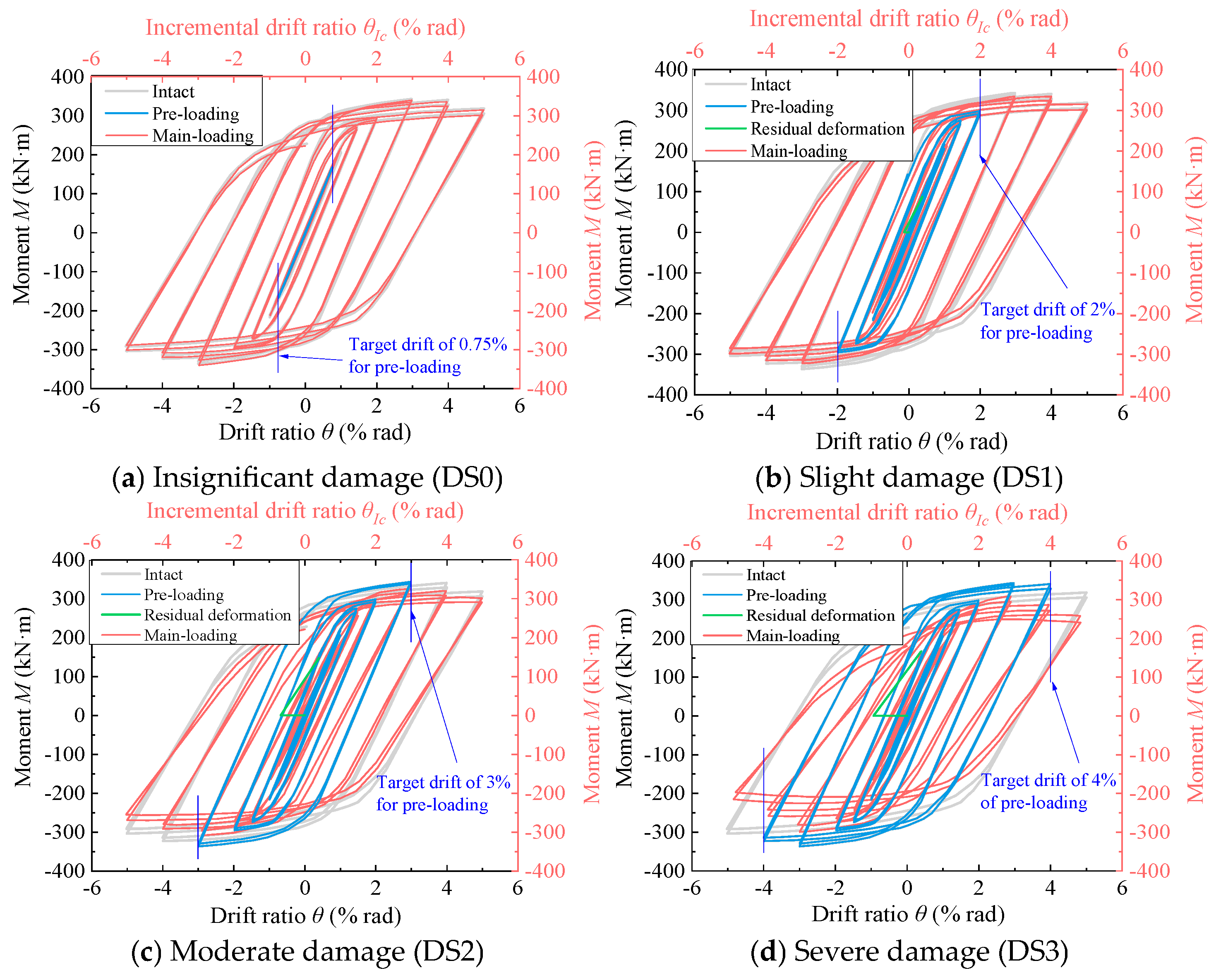
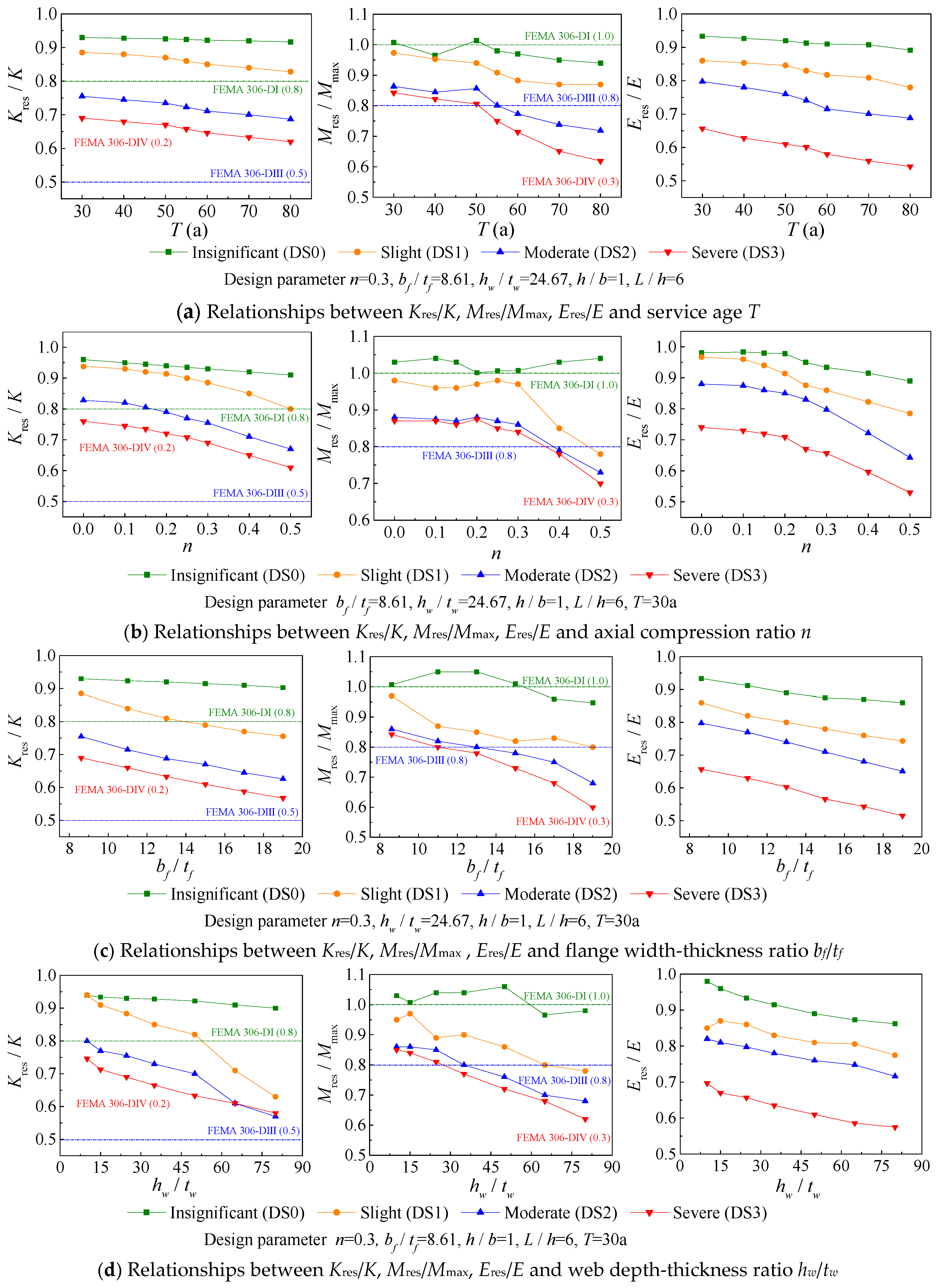
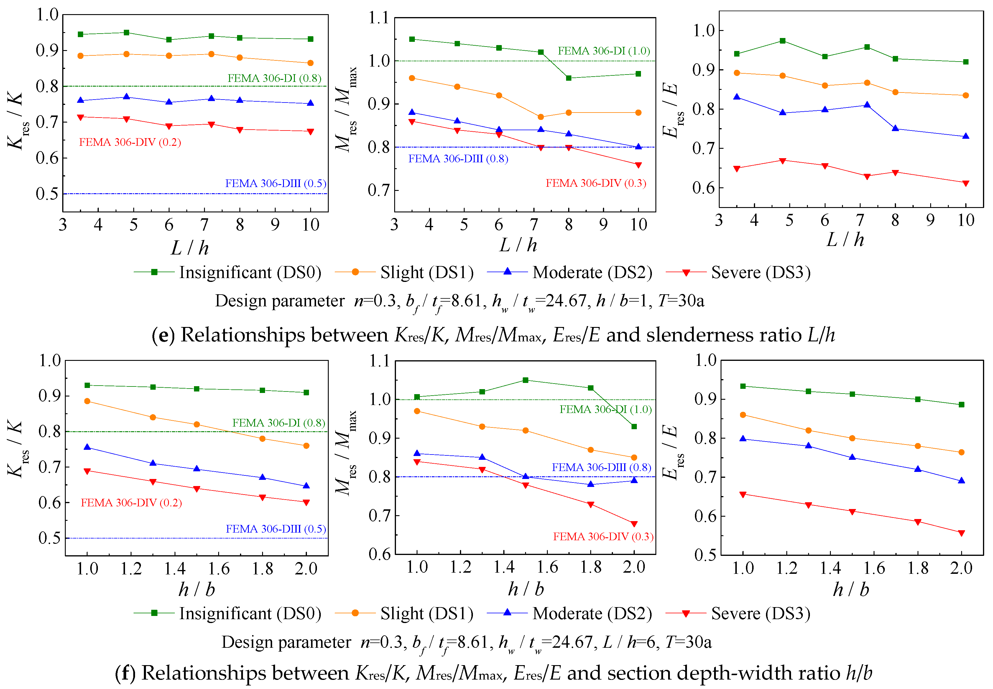
5.2. Residual Seismic Capacity Analysis
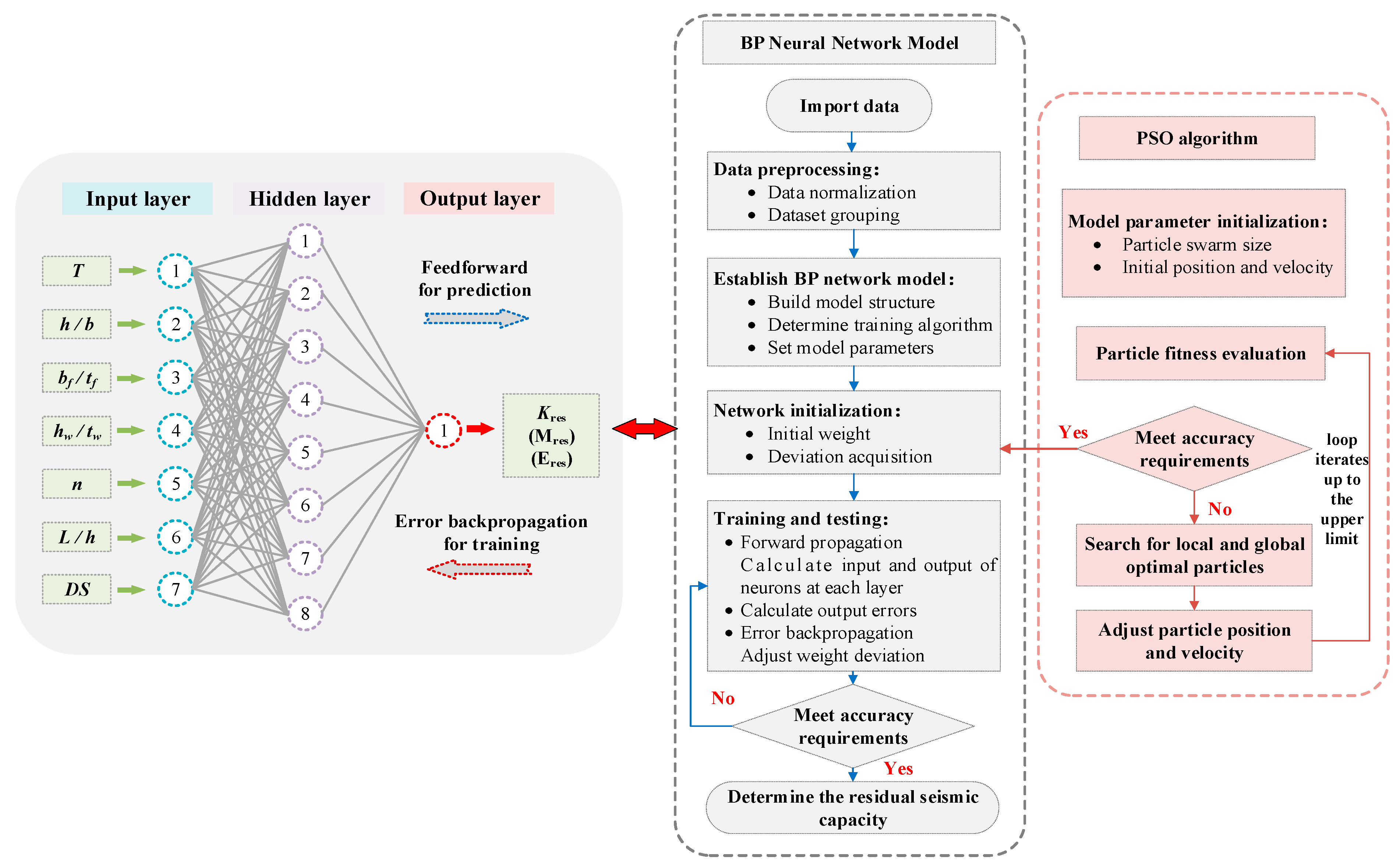
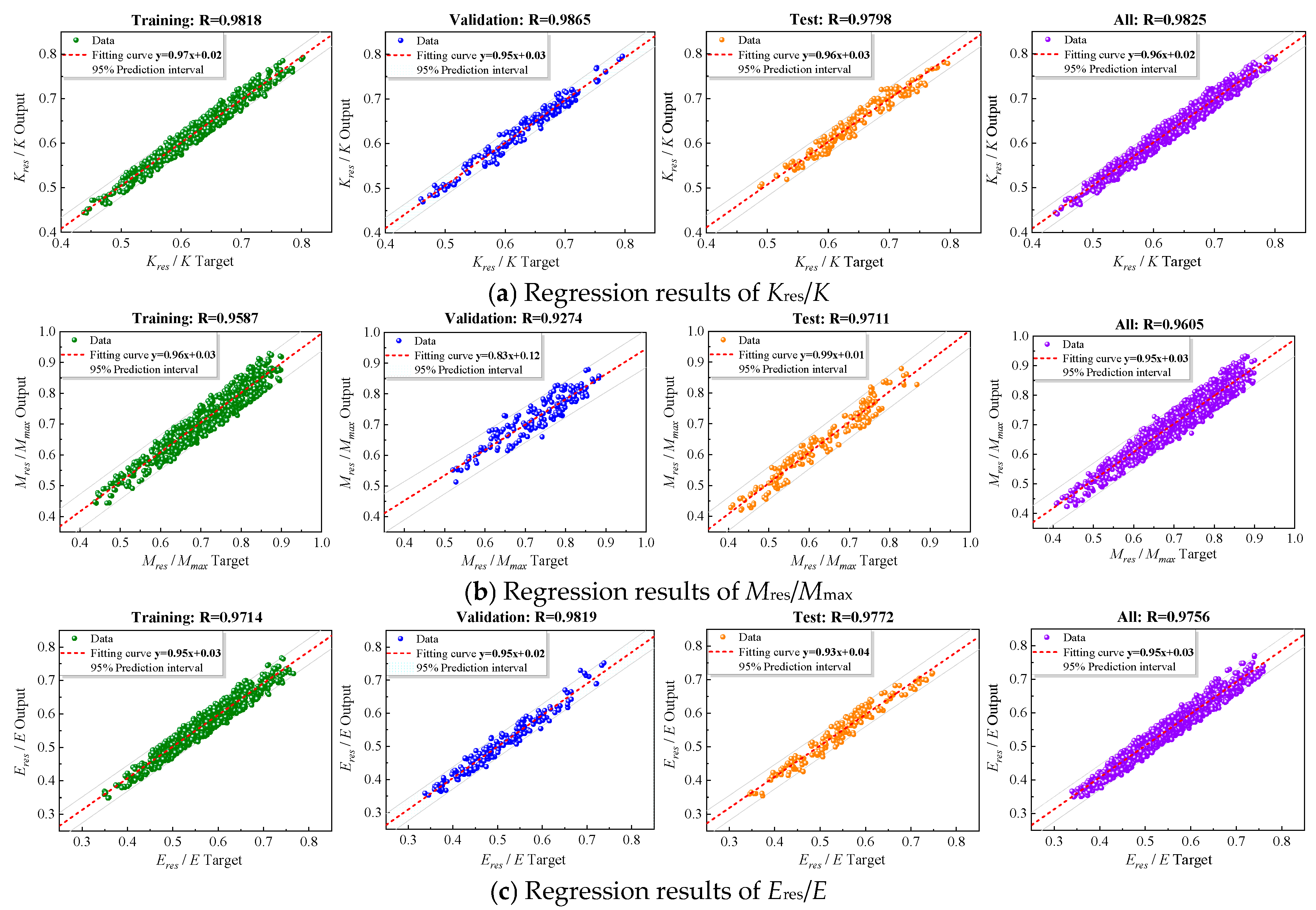
5.3. Implementation of PSO-BPNN Model
5.4. Residual Seismic Behavior Model
6. Conclusions
- (1)
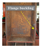
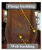
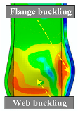
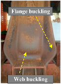
- With an increase in the corrosion level or axial compression ratio, the damage phenomena of steel column yielding, plate local buckling, and plastic hinge formation occurred prematurely, the bearing capacity decreased, and ductility and energy dissipation gradually deteriorated. Furthermore, an FEA method for steel frame columns considering corrosion damage and ductile metal damage criteria was developed and validated.
- (2)
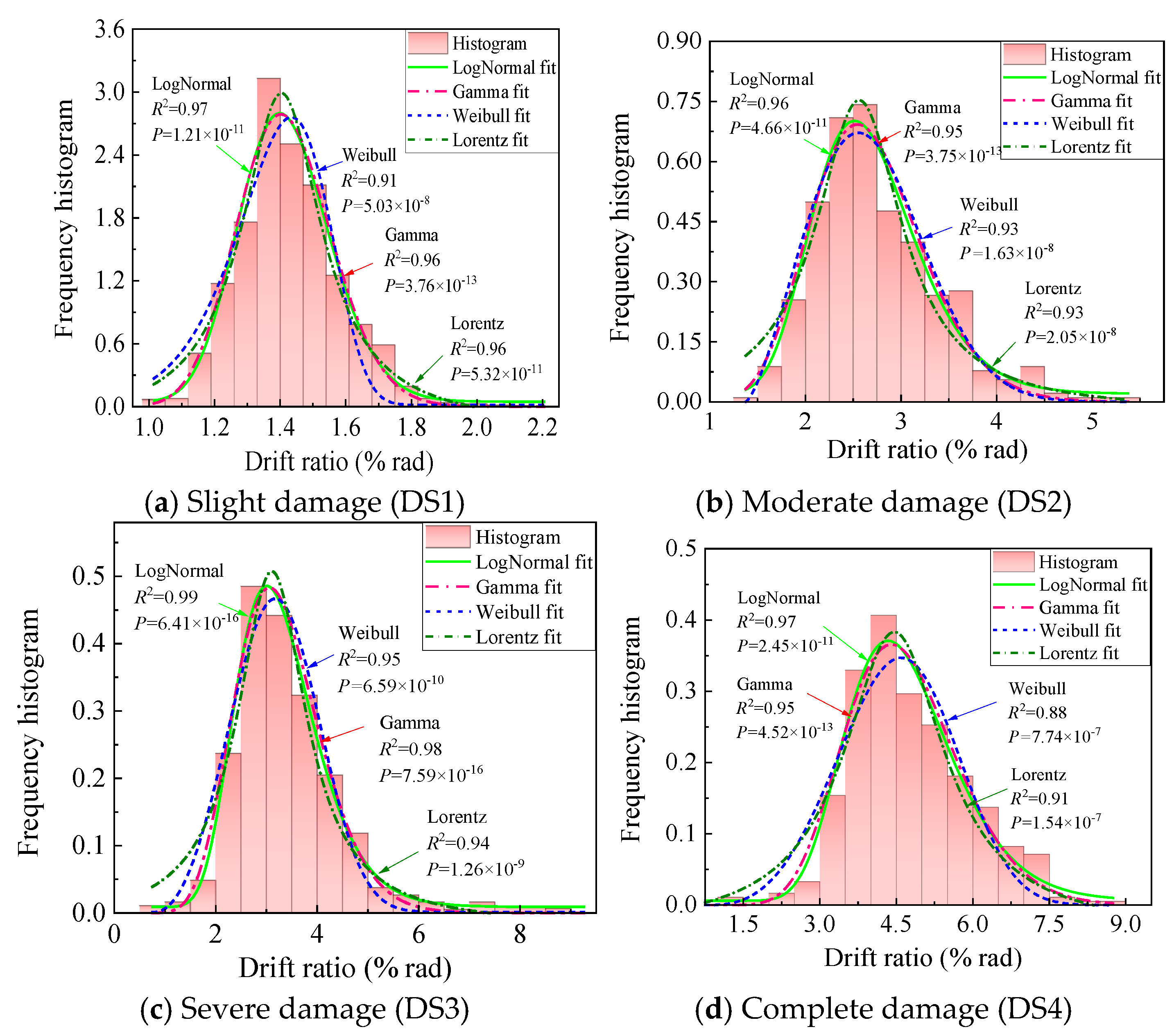
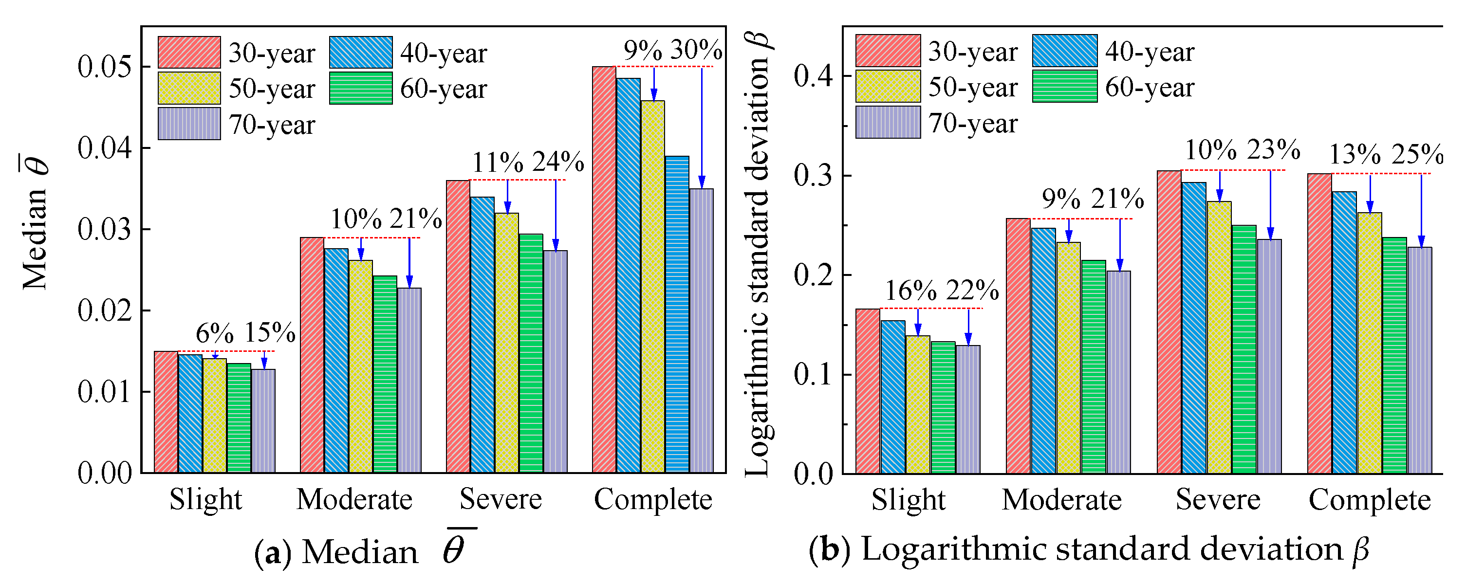
- Considering the impacts of environmental erosion and aging, a classification criterion and theoretical characterization of the damage states for existing steel frame columns were proposed. Thus, the probability distribution of the fragility function parameters (median and logarithmic standard deviation) was constructed, thereby presenting a time-dependent fragility model for existing steel frame columns in offshore atmospheric environments. At the drift ratio limit of 4% for SMFs in AISC 341-10, the probability matrices of complete damage to columns with 40, 50, 60, and 70-year service ages were 35.2%, 43.3%, 53.4%, and 66.9%, respectively, with increases of 18.1%, 45.3%, 79.2%, and 124.5%, respectively, compared with columns within 30-year service age (probability of 29.8%). These results indicate that existing steel components affected by environmental corrosion and aging undergo significant deterioration in seismic performance, and a feasible anti-corrosion measure with periodic maintenance should be introduced in practical seismic design.
- (3)
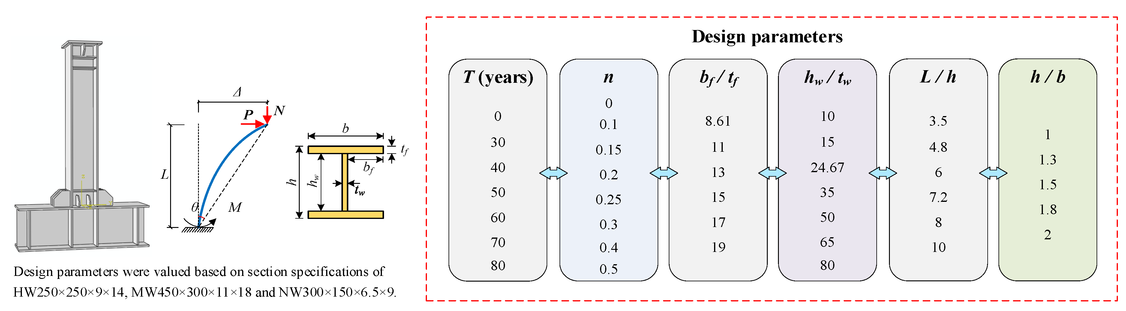
- Using the PSO-BPNN model, nonlinear mapping relationships between the characteristic variables, in terms of service age T, design parameters (n, bf/tf, hw/tw, L/h, and h/b), damage level, and residual seismic capability (Kres/K, Mres/Mmax, and Eres/E) for earthquake-damaged columns were constructed. Then, combined with the damage probability matrix of time-dependent fragility, the expected values of the residual seismic capacity for existing multi-aged steel frame columns at a given drift ratio can be presented directly in a probabilistic sense, achieving a scientific and efficient evaluation of the residual seismic behavior. For example, for 50-year-old steel frame columns (with the design parameters n = 0.3, bf/tf = 8.61, hw/tw = 24.67, h/b = 1, and L/h = 6), at a drift ratio limit of 4% for SMFs in AISC 341-10, the residual capacities Kres/K Mres/Mmax and Eres/E were 0.66, 0.79, and 0.63, respectively.
Author Contributions
Funding
Data Availability Statement
Conflicts of Interest
Appendix A
References
- Furley, J.; van de Lindt, J.W.; Pei, S.; Wichman, S.; Hasani, H.; Berman, J.W.; Ryan, K.; Dolan, J.D.; Zimmerman, R.B.; McDonnell, E. Time-to-Functionality Fragilities for Performance Assessment of Buildings. J. Struct. Eng. 2021, 147, 04021217. [Google Scholar] [CrossRef]
- Elwood, K.J.; Marquis, F.; Kim, J.H. Post-earthquake assessment and repairability of RC buildings: Lessons from canterbury and emerging challenges. In Proceedings of the Tenth Pacific Conference on Earthquake Engineering Building an Earthquake-Resilient Pacific, Sydney, Australia, 6–8 November 2015. [Google Scholar]
- UC Berkeley Pacific Earthquake Engineering Research Center (PEER). In Proceedings of the 2016 PEER Annual Meeting [EB/OL], Berkeley, CA, USA, 28–29 January 2016. Available online: https://peer.berkeley.edu/2016-peer-annual-meeting-presentations-website (accessed on 28 January 2016).
- Zhong, Z.; Fan, W.; Liu, B.; Huang, X.; Geng, B. A fragility-based framework for identification of unfavorable impact location for bridge columns under barge collisions. Ocean Eng. 2024, 294, 116839. [Google Scholar] [CrossRef]
- Applied Technology Council. Seismic Performance Assessment of Buildings, Volume 1—Methodology; Federal Emergency Management Agency: Washington, DC, USA, 2012.
- Goksu, C. Fragility functions for reinforced concrete columns incorporating recycled aggregates. Eng. Struct. 2021, 233, 111908. [Google Scholar] [CrossRef]
- Mohammadgholibeyki, N.; Epackachi, S. Fragility functions for steel-plate concrete composite shear walls. J. Constr. Steel Res. 2020, 167, 105776. [Google Scholar] [CrossRef]
- Wang, M.; Guo, Y.; Yang, L. Damage indices and fragility assessment of coupled low-yield-point steel plate shear walls. J. Build. Eng. 2021, 42, 103010. [Google Scholar] [CrossRef]
- Haghpanah, F.; Schafer, B.W. Updated seismic fragility functions for cold-formed steel framed shear walls per FEMA P-58 methodology. Eng. Struct. 2021, 244, 112753. [Google Scholar] [CrossRef]
- Zhang, H.; Liu, H.; Deng, Y.; Cao, Y.; He, Y.; Liu, Y.; Deng, Y. Fatigue behavior of high-strength steel wires considering coupled effect of multiple corrosion-pitting. Corros. Sci. 2024, 244, 112633. [Google Scholar] [CrossRef]
- Zhang, H.; Deng, Y.; Cao, Y.; Chen, F.; Luo, Y.; Xiao, X.; Deng, Y.; Liu, Y. Field testing, analytical, and numerical assessments on the fatigue reliability on bridge suspender by considering the coupling effect of multiple pits. Struct. Infrastruct. Eng. 2025, 1–16. [Google Scholar] [CrossRef]
- Mirzaeefard, H.; Hariri-Ardebili, M.A.; Mirtaheri, M. Time-dependent seismic fragility analysis of corroded pile-supported wharves with updating limit states. Soil Dyn. Earthq. Eng. 2021, 142, 106551. [Google Scholar] [CrossRef]
- Zhao, X.; Zhang, X.; Zheng, S.; Yang, Q. Residual seismic performance and fragility assessment of corroded steel beam-column welded joints. Structures 2025, 73, 108455. [Google Scholar] [CrossRef]
- Zhang, B.; Wang, K.; Lu, G.; Guo, W.; Liu, J.; Zhang, N.; Yang, C. Life-cycle seismic performance analysis of an offshore small-to-medium span bridge based on interpretable machine learning. Structures 2024, 70, 107511. [Google Scholar] [CrossRef]
- Xu, B.; Wang, X.; Yang, C.-S.W.; Li, Y. Machine Learning–Aided Rapid Estimation of Multilevel Capacity of Flexure-Identified Circular Concrete Bridge Columns with Corroded Reinforcement. J. Struct. Eng. 2024, 150, 04024002. [Google Scholar] [CrossRef]
- Fu, B.; Feng, D.-C. A machine learning-based time-dependent shear strength model for corroded reinforced concrete beams. J. Build. Eng. 2021, 36, 102118. [Google Scholar] [CrossRef]
- Gutiérrez-Urzúa, F.; Freddi, F.; Di Sarno, L. Comparative analysis of code-based approaches for seismic assessment of existing steel moment resisting frames. J. Constr. Steel Res. 2021, 181, 106589. [Google Scholar] [CrossRef]
- Zahra, F.; Macedo, J.; Málaga-Chuquitaype, C. The importance of hazard-consistency when estimating seismic residual drifts in steel moment frames. J. Build. Eng. 2024, 84, 108506. [Google Scholar] [CrossRef]
- Japan Building Disaster Prevention Association. Standard for Postearthquake Damage Level Classification of Buildings; Japan Building Disaster Prevention Association: Tokyo, Japan, 2016. (In Japanese) [Google Scholar]
- FEMA-306; Evaluation of Earthquake Damaged Concrete and Masonry Wall Buildings—Basic Procedures Manual. Federal Emergency Management Agency: Washington, DC, USA, 1999.
- Alwashali, H.; Maeda, M.; Ogata, Y.; Aizawa, N.; Tsurugai, K. Residual seismic performance of damaged reinforced concrete walls. Eng. Struct. 2021, 243, 112673. [Google Scholar] [CrossRef]
- Harrington, C.C.; Liel, A.B. Evaluation of Seismic Performance of Reinforced Concrete Frame Buildings with Retrofitted Columns. J. Struct. Eng. 2020, 146, 04020237. [Google Scholar] [CrossRef]
- Khanmohammadi, M.; Kharrazi, H. Residual Capacity of Mainshock-Damaged Precast-Bonded Prestressed Segmental Bridge Deck under Vertical Earthquake Ground Motions. J. Bridg. Eng. 2018, 23, 04018016. [Google Scholar] [CrossRef]
- Chiu, C.K.; Sung, H.F.; Chi, K.N.; Hsiao, F.P. Experimental quantification on the residual seismic capacity of damaged RC column members. Int. J. Concr. Struct. Mater. 2019, 13, 17. [Google Scholar] [CrossRef]
- Zhang, Y.; Burton, H.V. Pattern recognition approach to assess the residual structural capacity of damaged tall buildings. Struct. Saf. 2019, 78, 12–22. [Google Scholar] [CrossRef]
- Cavaleri, L.; Zizzo, M.; Asteris, P.G. Residual out-of-plane capacity of infills damaged by in-plane cyclic loads. Eng. Struct. 2020, 209, 109957. [Google Scholar] [CrossRef]
- Asgarkhani, N.; Kazemi, F.; Jankowski, R. Machine learning-based prediction of residual drift and seismic risk assessment of steel moment-resisting frames considering soil-structure interaction. Comput. Struct. 2023, 289, 107181. [Google Scholar] [CrossRef]
- GB 50011-2010; Code for Seismic Design of Buildings. Architecture & Building Press: Beijing, China, 2010. (In Chinese)
- GB 50017-2017; Code for Design of Steel Structures. China Planning Press: Beijing, China, 2017. (In Chinese)
- ISO 9227: 2017; Corrosion Tests in Artificial Atmospheres—Salt Spray Tests. International Organization for Standardization: Geneva, Switzerland, 2017.
- Zhang, X.; Zheng, S.; Zhao, X. Experimental and numerical investigations into seismic behavior of corroded steel frame beams and columns in offshore atmospheric environment. J. Constr. Steel Res. 2022, 201, 107757. [Google Scholar] [CrossRef]
- Yu, H.; Jeong, D. Application of a stress triaxiality dependent fracture criterion in the finite element analysis of unnotched Charpy specimens. Theor. Appl. Fract. Mech. 2010, 54, 54–62. [Google Scholar] [CrossRef]
- Wierzbicki, T.; Bao, Y.; Lee, Y.-W.; Bai, Y. Calibration and evaluation of seven fracture models. Int. J. Mech. Sci. 2005, 47, 719–743. [Google Scholar] [CrossRef]
- ASCE/SEI 41-06; Seismic Rehabilitation of Existing Buildings. American Society of Civil Engineers: Reston, VA, USA, 2007.
- FEMA 356; Prestandard and Commentary for the Seismic Rehabilitation of Buildings. Federal Emergency Management Agency: Washington, DC, USA, 2000.
- EN1998-3; Eurocode 8-Design of Structures for Earthquake Resistance-Part 3: Assessment and Retrofitting of Buildings. European standards: Brussels, Belgium, 2005.
- Hazus-MH MR5; Earthquake Loss Estimation Methodology—Technical and User’s Manual. Department of Homeland Security, Federal Emergency Management Agency, Mitigation Division: Washington, DC, USA, 2010.
- GB/T 38591-2020; Standard for Seismic Resilience Assessment of Buildings. China Standards Press: Beijing, China, 2020. (In Chinese)
- IS012944-2; 2017 Paints and Varnishes—Corrosion Protection of Steel Structures by Protective Paint Systems—Part 2: Classification of environments. International Organization for Standardization: Geneva, Switzerland, 2017.
- GB/T 50046-2018; Standard for Anticorrosion Design of Industrial Constructions. China Planning Press: Beijing, China, 2018. (In Chinese)
- Garbatov, Y.; Soares, C.G.; Wang, G. Nonlinear Time Dependent Corrosion Wastage of Deck Plates of Ballast and Cargo Tanks of Tankers. J. Offshore Mech. Arct. Eng. 2006, 129, 48–55. [Google Scholar] [CrossRef]
- Wang, Y.; Wharton, J.; Shenoi, R. Mechano-electrochemical modelling of corroded steel structures. Eng. Struct. 2016, 128, 1–14. [Google Scholar] [CrossRef]
- Zhang, X.; Zheng, S.; Zhao, X. Experimental and numerical study on seismic performance of corroded steel frames in chloride environment. J. Constr. Steel Res. 2020, 171, 106164. [Google Scholar] [CrossRef]
- D’Ayala, D.; Meslem, A.; Vamvatsikos, D.; Porter, K.; Rossetto, T.; Crowley, H.; Silva, V. Guidelines for analytical vulnerability assessment of low-mid-rise buildings -methodology. Utop. Stud. 2014, 25, 150–173. [Google Scholar]
- Zhang, X.; Zheng, S.; Zhao, X.; Yang, Q. Seismic performance and hysteretic model of corroded steel frame columns in offshore atmospheric environment. Adv. Struct. Eng. 2023, 26, 3041–3064. [Google Scholar] [CrossRef]
- ANSI/AISC 341-10; Seismic Provisions for Structural Steel Buildings. American Institute of Steel Construction: Chicago, IL, USA, 2010.
- Xiao, M.; Luo, R.; Chen, Y.; Ge, X. Prediction model of asphalt pavement functional and structural performance using PSO-BPNN algorithm. Constr. Build. Mater. 2023, 407, 133534. [Google Scholar] [CrossRef]
- Cai, B.; Lin, X.; Fu, F.; Wang, L. Postfire residual capacity of steel fiber reinforced volcanic scoria concrete using PSO-BPNN machine learning. Structures 2022, 44, 236–247. [Google Scholar] [CrossRef]
- Hu, S.; Lei, X. Machine learning and genetic algorithm-based framework for the life-cycle cost-based optimal design of self-centering building structures. J. Build. Eng. 2023, 78, 107671. [Google Scholar] [CrossRef]

| Related Studies | Novelty of the Studies | |||||
|---|---|---|---|---|---|---|
| Component Seismic Fragility (Yes or No) | Post-Earthquake Residual Seismic Behavior (Yes or No) | Environmental Corrosion and Aging Impact (Yes or No) | Machine Learning Techniques (Yes or No) | Relationships Between the Damage Characteristics and Residual Seismic Capacity (Yes or No) | Structural Variable Parameters (Yes or No) | |
| Literature [5] | Yes | No | No | No | No | Yes |
| Literature [6,7,8,9] | Yes | No | No | No | No | Yes |
| Literature [12,13] | Yes | No | Yes | No | No | Yes |
| Literature [14,15,16] | Yes | No | Yes | Yes | No | Yes |
| Literature [19,20] | No | Yes | No | No | Yes | Yes |
| Literature [21,22,23,24,26] | No | Yes | No | No | Yes | No |
| Literature [25,27] | No | Yes | No | No | Yes | Yes |
| This study | Yes | Yes | Yes | Yes | Yes | Yes |
| Specimen No. | Section Specification (mm) | Axial Compression Ratio n | Accelerated Corrosion Time t (h) | Mass Loss Rate η (%) |
|---|---|---|---|---|
| SFC-1 | HW 250 × 250 × 9 × 14 | 0.3 | 0 | 0.00 |
| SFC-2 | HW 250 × 250 × 9 × 14 | 0.3 | 960 | 3.06 |
| SFC-3 | HW 250 × 250 × 9 × 14 | 0.3 | 1920 | 5.33 |
| SFC-4 | HW 250 × 250 × 9 × 14 | 0.3 | 2880 | 8.02 |
| SFC-5 | HW 250 × 250 × 9 × 14 | 0.2 | 1920 | 5.33 |
| SFC-6 | HW 250 × 250 × 9 × 14 | 0.4 | 1920 | 5.33 |
| Specimen No. | Drift Ratio Level of Flange Local Buckling | Drift Ratio Level of Web Local Buckling | Drift Ratio Level of Maximum Load | Drift Ratio Level of Failure | Plastic Hinge Length (mm) | Failure Mode of Cross Section | Damage State | |||
|---|---|---|---|---|---|---|---|---|---|---|
| DS1 | DS2 | DS3 | DS4 | |||||||
| SFC-1 | 3% (2) | 4% (2) | 4% (1) | 5% (2) | 340 |  | 1.60% | 2.62% | 3.13% | 4.79% |
| SFC-2 | 3% (2) | 4% (1) | 3% (2) | 5% (1) | 325 | 1.54% | 2.51% | 3.00% | 4.49% | |
| SFC-3 | 3% (1) | 4% (1) | 3% (2) | 5% (1) | 315 | 1.47% | 2.48% | 2.99% | 3.96% | |
| SFC-4 | 2% (2) | 3% (1) | 3% (1) | 4% (2) | 330 | 1.37% | 2.36% | 2.86% | 3.67% | |
| SFC-5 | 3% (2) | 4% (2) | 4% (1) | 5% (2) | 330 | 1.64% | 3.21% | 4.00% | 4.99% | |
| SFC-6 | 2% (2) | 3% (2) | 3% (1) | 4% (2) | 280 | 1.42% | 2.43% | 2.94% | 3.82% | |
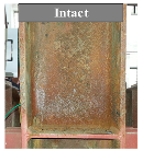
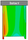
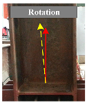
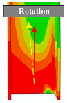
| Damage States | Description of Damage Phenomena | Repair Methods | Visual Illustrations | |
|---|---|---|---|---|
| Insignificant (DS0) |
|
|  |  |
| Slight (DS1) |
|
|  |  |
| Moderate (DS2) |
|
|  |  |
| Severe (DS3) |
|
|  |  |
| Complete (DS4) |
|
|  |  |
| Service Age | Damage ID | Fragility Function Parameters | Lilliefors Test | |||
|---|---|---|---|---|---|---|
| β | D | Dcrit | Result | |||
| 30 years | Slight (DS1) | 0.0150 | 0.166 | 0.035 | 0.046 | Pass |
| Moderate (DS2) | 0.0290 | 0.257 | 0.038 | Pass | ||
| Severe (DS3) | 0.0360 | 0.305 | 0.049 | Fail | ||
| Complete (DS4) | 0.0500 | 0.302 | 0.044 | Pass | ||
| 40 years | Slight (DS1) | 0.0146 | 0.154 | 0.040 | Pass | |
| Moderate (DS2) | 0.0276 | 0.247 | 0.028 | Pass | ||
| Severe (DS3) | 0.0340 | 0.293 | 0.052 | Fail | ||
| Complete (DS4) | 0.0486 | 0.284 | 0.043 | Pass | ||
| 50 years | Slight (DS1) | 0.0141 | 0.139 | 0.029 | Pass | |
| Moderate (DS2) | 0.0262 | 0.233 | 0.038 | Pass | ||
| Severe (DS3) | 0.0320 | 0.274 | 0.066 | Fail | ||
| Complete (DS4) | 0.0458 | 0.263 | 0.047 | Fail | ||
| 60 years | Slight (DS1) | 0.0135 | 0.133 | 0.032 | Pass | |
| Moderate (DS2) | 0.0243 | 0.215 | 0.04 | Pass | ||
| Severe (DS3) | 0.0294 | 0.250 | 0.058 | Fail | ||
| Complete (DS4) | 0.0390 | 0.238 | 0.054 | Fail | ||
| 70 years | Slight (DS1) | 0.0128 | 0.129 | 0.034 | Pass | |
| Moderate (DS2) | 0.0228 | 0.204 | 0.036 | Pass | ||
| Severe (DS3) | 0.0274 | 0.236 | 0.044 | Pass | ||
| Complete (DS4) | 0.0350 | 0.228 | 0.050 | Fail | ||
| Current Specifications | Category | Damage States-Median Demand () | |||
|---|---|---|---|---|---|
| This study (30 years) | Steel frame column | DS1 | DS2 | DS3 | DS4 |
| 0.015 | 0.029 | 0.036 | 0.050 | ||
| FEMA P-58 [5] | Column Base Plates | DS1 | DS2 | DS3 | |
| 0.04 (strong axis) | 0.07(strong axis) | 0.10(strong axis) | |||
| non-RBS Beam-Column Moment Connections | DS1 | DS2 | DS3 | ||
| 0.03 | 0.04 | 0.05 | |||
| HAZUS [37] | Steel moment frame | Slight | Moderate | Extensive | Complete |
| 0.003 | 0.006 | 0.015 | 0.040 | ||
| FEMA 356 [35] | Steel structures | IO | LS | CP | |
| 0.007 | 0.025 | 0.050 | |||
| GB 50011-2010 [28] | Steel structure vertical component | Basically intact | Slight | Moderate | Extensive |
| 0.003 | 0.005 | 0.01 | 0.018 | ||
| GB/T 38591-2022 [38] | Steel column (0.3 < n < 0.5) | IO | K | LS | CP |
| 1.25 θy | (8.125–11.7 n) θy | (15–23.3 n) θy | (18–28.3 n) θy | ||
| Damage ID | Regression Coefficients | |||
|---|---|---|---|---|
| Logarithmic Standard Deviation β | ||||
| Slight (DS1) | 0.017 | −5.50 × 10⁻⁵ | 0.192 | −9.50 × 10⁻⁴ |
| Moderate (DS2) | 0.034 | −1.57 × 10⁻⁴ | 0.300 | −1.38 × 10⁻³ |
| Severe (DS3) | 0.043 | −2.18 × 10⁻⁴ | 0.362 | −1.81 × 10⁻³ |
| Complete (DS4) | 0.063 | −3.96 × 10⁻⁴ | 0.360 | −1.94 × 10⁻³ |
| Damage ID | Pre-Loading | |||||||||
|---|---|---|---|---|---|---|---|---|---|---|
| Drift Ratio θ and Cycle Number | ||||||||||
| ±0.375% | ±0.5% | ±0.75% | ±1% | ±1.5% | ±2% | ±3% | ±4% | |||
| DS0 | 2 | 2 | 5 | |||||||
| DS1 | 2 | 2 | 2 | 2 | 2 | 5 | ||||
| DS2 | 2 | 2 | 2 | 2 | 2 | 2 | 5 | |||
| DS3 | 2 | 2 | 2 | 2 | 2 | 2 | 2 | 5 | ||
| ID | Main-loading | |||||||||
| Incremental drift ratio θIc and cycle number | ||||||||||
| ±0.375% | ±0.5% | ±0.75% | ±1% | ±1.5% | ±2% | ±3% | ±4% | ±5% | … | |
| DS0–DS3 | 2 | 2 | 2 | 2 | 2 | 2 | 2 | 2 | 2 | 2 |
| Performance Indicators | Kres/K | Mres/Mmax | Eres/E | |
|---|---|---|---|---|
| R2 | Training set | 0.9638 | 0.9191 | 0.9437 |
| Validation set | 0.9732 | 0.8601 | 0.9642 | |
| Testing set | 0.9599 | 0.9430 | 0.9550 | |
| All dataset | 0.9653 | 0.9225 | 0.9518 | |
| RMSE | Training set | 0.0129 | 0.0291 | 0.0200 |
| Validation set | 0.0115 | 0.0331 | 0.0170 | |
| Testing set | 0.0130 | 0.0269 | 0.0190 | |
| All dataset | 0.0127 | 0.0294 | 0.0194 | |
Disclaimer/Publisher’s Note: The statements, opinions and data contained in all publications are solely those of the individual author(s) and contributor(s) and not of MDPI and/or the editor(s). MDPI and/or the editor(s) disclaim responsibility for any injury to people or property resulting from any ideas, methods, instructions or products referred to in the content. |
© 2025 by the authors. Licensee MDPI, Basel, Switzerland. This article is an open access article distributed under the terms and conditions of the Creative Commons Attribution (CC BY) license (https://creativecommons.org/licenses/by/4.0/).
Share and Cite
Zhang, X.; Zhao, X.; Zheng, S.; Yang, Q. Time-Dependent Fragility Functions and Post-Earthquake Residual Seismic Performance for Existing Steel Frame Columns in Offshore Atmospheric Environment. Buildings 2025, 15, 2330. https://doi.org/10.3390/buildings15132330
Zhang X, Zhao X, Zheng S, Yang Q. Time-Dependent Fragility Functions and Post-Earthquake Residual Seismic Performance for Existing Steel Frame Columns in Offshore Atmospheric Environment. Buildings. 2025; 15(13):2330. https://doi.org/10.3390/buildings15132330
Chicago/Turabian StyleZhang, Xiaohui, Xuran Zhao, Shansuo Zheng, and Qian Yang. 2025. "Time-Dependent Fragility Functions and Post-Earthquake Residual Seismic Performance for Existing Steel Frame Columns in Offshore Atmospheric Environment" Buildings 15, no. 13: 2330. https://doi.org/10.3390/buildings15132330
APA StyleZhang, X., Zhao, X., Zheng, S., & Yang, Q. (2025). Time-Dependent Fragility Functions and Post-Earthquake Residual Seismic Performance for Existing Steel Frame Columns in Offshore Atmospheric Environment. Buildings, 15(13), 2330. https://doi.org/10.3390/buildings15132330