Integrated Wavelet-Grey-Neural Network Model for Heritage Structure Settlement Prediction

Abstract

To address the issue of insufficient prediction accuracy in traditional GM(1,1) models caused by significant nonlinear fluctuations in time-series data for ancient building structural health monitoring, this study proposes a wavelet decomposition-based GM(1,1)-BP neural network coupled prediction model. By constructing a multi-scale fusion framework, we systematically resolve the collaborative optimization between trend prediction and detail modeling. The methodology comprises four main phases: First, wavelet transform is employed to decompose original monitoring sequences into time-frequency components, obtaining low-frequency trends characterizing long-term deformation patterns and high-frequency details reflecting dynamic fluctuations. Second, GM(1,1) models are established for the trend extrapolation of low-frequency components, capitalizing on their advantages in limited-data modeling. Subsequently, BP neural networks are designed for the nonlinear mapping of high-frequency components, leveraging adaptive learning mechanisms to capture detail features induced by environmental disturbances and complex factors. Finally, a wavelet reconstruction fusion algorithm is developed to achieve the collaborative optimization of dual-channel prediction results. The model innovatively introduces a detail information correction mechanism that simultaneously overcomes the limitations of single grey models in modeling nonlinear fluctuations and enhances neural networks’ capability in capturing long-term trend features. Experimental validation demonstrates that the fused model reduces the Root Mean Square Error (RMSE) by 76.5% and 82.6% compared to traditional GM(1,1) and BP models, respectively, with the accuracy grade improving from level IV to level I. This achievement provides a multi-scale analytical approach for the quantitative interpretation of settlement deformation patterns in ancient architecture. The established “decomposition-prediction-fusion” technical framework holds significant application value for the preventive conservation of historical buildings.

1. Introduction

As material carriers of historical and cultural heritage, heritage structures face multiple threats to their structural safety and long-term preservation, including natural weathering, environmental erosion, and anthropogenic disturbances [1]. In the preventive conservation system, deformation monitoring and prediction techniques serve as core methods. By acquiring real-time deformation data on main structures and conducting trend analysis, these techniques can effectively identify potential safety hazards and provide a basis for scientific decision making.

In the field of cultural heritage conservation, the health monitoring of heritage structures faces multiple challenges, including significant data noise interference, prominent sample scarcity, and coexisting data complexity and uncertainty. Owing to its unique modeling advantages for small-sample and poor-information systems, Grey System Theory has demonstrated important application value in deformation monitoring and analysis [2]. In recent years, Jiang et al. [3] pointed out that due to its linear assumption, the classical grey model faces challenges when dealing with complex nonlinear data. They proposed an improved grey model with a time power term. Huang et al. [4] indicated that grey models (such as GM(1,1)) have strict requirements for the smoothness of input data. If the original data fluctuates greatly, the prediction accuracy will significantly decline. Kankanamge [5] combined wavelet decomposition to process non-stationary signals and achieved good results in the health monitoring of wooden structures. Comert et al. [6] pointed out that traditional grey models assume that the system changes monotonically in an exponential manner and cannot capture nonlinear relationships. They used Bayesian optimization of parameters to improve the noise-resistance ability of the model. Deep learning techniques have been widely applied in the field of Structural Health Monitoring (SHM) due to their strong nonlinear modeling capabilities. Convolutional Neural Networks (CNNs) and Long Short-Term Memory Networks (LSTMs) are widely used in vibration signal analysis and damage identification. For example, Wang et al. [7] proposed a new method for bridge damage identification using encoded images and CNNs, which significantly improved the identification accuracy. Similarly, Yun et al. [8] proposed an adaptive Stochastic Subspace Identification-Long Short-Term Memory (SSI-LSTM) method. By applying it to the response data of a 55-story high-rise building, they verified the effectiveness of LSTM in processing time-series data on building structures and analyzing their structural dynamic characteristics. Fadel et al. [9] proposed a new CNN-LSTM structure based on classification and regression for bridge damage identification, considering the influence of temperature. This model outperforms conventional CNN models and traditional machine learning algorithms in bridge damage identification. In addition, Chaiyasarn et al. [10] proposed an automatic crack detection system for masonry structures based on CNNs, which is used for crack identification in masonry buildings. These studies show that deep learning has great potential for settlement prediction, but the generalization problem with small-sample data still needs to be solved. The damage identification of long-span structures is another important research direction in the field of structural health monitoring. For example, Feng et al. [11] proposed a stiffness separation method for beam-bridge parameter identification and verified the accuracy and efficiency of the proposed method through continuous beam bridges. Li et al. [12] used a one-dimensional Convolutional Neural Network (1DCNN) to detect internal damage in aluminum plates. The proposed method achieved a 96% accuracy rate in damage identification, significantly improving the sensitivity of early damage identification. Sun et al. [13] proposed a method for damage detection in steel-truss bridges using Gaussian Bayesian Networks (GBNs). Through numerical simulations of an 80-meter steel-truss bridge, this method can accurately predict stress and detect damage in steel-truss bridges. Morteza et al. [14] adopted a new method called Frugal Wavelet Transform (FrugWT) to study the damage detection problem of composite laminated beams, and was able to accurately detect damage at different positions in the laminated beams (LCBs). Vahid et al. [15] proposed a data-augmentation strategy based on a Transformer-based Time-Series Wasserstein Generative Adversarial Network for bridge infrastructure, reducing the dependence on large-scale data collection. Although these methods perform well in modern structures such as bridges, their applicability in the field of ancient architecture still needs to be verified. Mallat [16] pointed out that wavelet transform can effectively decompose non-stationary signals, while grey models are suitable for small-sample prediction [2]. Ma et al. [17] proposed a combination of wavelet packet analysis and neural networks, and put forward a new method for structural damage localization under variable-temperature conditions. Even in the case of noise interference, this method can accurately detect and locate structural damage under different temperature conditions. Li et al. [18] addressed the problem of large deviations in the linear prediction of long-span continuous beam bridges by grey prediction models. They proposed a bridge camber prediction method based on the combination of a grey model (GM) and a Back-Propagation neural network (GM-BP). When the data is limited and irregular, the GM-BP combined prediction model has high prediction accuracy and stability. Hao et al. [19] proposed a CNN-LSTM neural network model for the high-precision prediction of real-time seismic responses in soil-tunnel structures. Compared with single models, the CNN-LSTM hybrid network can effectively predict the real-time seismic response at any time, with higher accuracy and robustness.

This study proposes a coupled prediction model of a GM(1,1)-BP neural network based on wavelet transform. A wavelet decomposition layer is introduced to enhance the analytical ability of the prediction model for non-stationary signals. The interpretability of the model with small samples is retained through the grey model, avoiding the problem of unstable training caused by insufficient data in deep learning models [20]. Furthermore, a BP neural network is introduced to perform refined modeling on the high-frequency components instead of directly discarding or simply smoothing them, so as to more accurately reflect their short-term dynamic characteristics. The BP neural network has a stronger nonlinear fitting ability and does not need to rely on the selection of kernel functions, making it more suitable for learning the complex patterns of high-frequency details. This makes up for the deficiencies of a single model in terms of its nonlinear prediction, adaptability to small samples, and detailed information. Specifically, the wavelet transform is used to decompose the monitoring signal in the time-frequency domain to obtain the low-frequency trend term representing the long-term law, and the high-frequency detail term reflecting the local dynamic characteristics. Then, the grey GM(1,1) model is used to perform trend extrapolation prediction on the low-frequency components, giving full play to its modeling advantages for systems with poor information. At the same time, the BP neural network is used to perform nonlinear fitting on the high-frequency components, effectively capturing the detailed fluctuations caused by complex factors such as environmental disturbances. By establishing the fusion algorithm in this paper, the dynamic coupling of the prediction results of the two channels is realized, forming a prediction model with “trend-detail” collaborative optimization.

2. Principles and Methods

2.1. Wavelet Multiscale Decomposition

Multiresolution analysis is to gradually decompose the signal into subspaces of different resolutions and achieve the fine extraction of signal features through a multi-scale decomposition mechanism [16].

Let $W_j$ be the orthogonal complement space of $V_j$, that is, $V_{j+1}=V_j\oplus W_j$. Then the signal space $L^2\left(R\right)$ can be expressed as:

$$L^2(R)=\dots \oplus W_{-1}\oplus W_0\oplus W_1\oplus \cdots$$

(1)

This means that the signal is decomposed at different resolutions. First, the signal is decomposed into the coarsest resolution subspace $V_j$ ($j$ is a given integer), and then the detail information is gradually decomposed into each $W_j$ space. Specifically, for any function $f(t)\in L^2\left(R\right)$, it can be decomposed into a detailed part and a large-scale part. The large-scale part can be further decomposed. Using the Mallat algorithm, the signal is decomposed into different frequency parts:

$$f(t)=A_{J}f(t)+{\displaystyle \sum _{j=J+1}{D}_{j}f(t)},$$

(2)

Among them, $A_{J}f(t)$ is the approximation, and $D_{j}f(t)$ is the detailed information of the signal at resolution $J$.

Wavelet multiresolution analysis can decompose the signal at different resolutions or scales, providing a multi-dimensional perspective for signal analysis. At a coarse scale, the overall characteristics and trends of the signal can be grasped; while at a fine scale, the detailed information of the signal can be captured, and the detailed information containing key local characteristics can be accurately obtained.

2.2. Grey Model

As a key methodology for modeling poor-information systems, Grey System Theory (GST) focuses on revealing the evolutionary laws of systems through limited information [21]. Grey Models (GMs) target small-sample, uncertain systems with ‘partially known and partially unknown information’, reconstructing the intrinsic characteristics of data through generation processing techniques to overcome the dependence of traditional statistical methods on large datasets. As a typical paradigm in Grey Prediction Theory, the GM(1,1) model dynamically describes system behavior by constructing a first-order single-variable differential equation. Its modeling process primarily includes the following steps:

Let the non-negative observation data of a deformation object be $X^{(0)}=\left\{X(i),i=1,2,\dots n\right\}$. First, an accumulative generation operation (AGO) is applied to the original sequence to obtain a new sequence $X^{(1)}$:

$$X^{(1)}(\mathrm{k})={\displaystyle \sum _{\mathrm{i}=1}^{\mathrm{k}}{X}^{(0)}}(i)=X^{(1)}(\mathrm{k}-1)+X^{(0)}(\mathrm{k})$$

(3)

This accumulation weakens random disturbances and strengthens deterministic patterns [22]. Next, a grey differential equation is established to reveal the system’s evolutionary trend, forming the GM(1,1) model:

$${\displaystyle \frac{\mathrm{d}{X}^{(1)}}{d_t}}+a{X}^{(1)}=b$$

(4)

where parameters $a,b$ are determined by ${(a,b)}^T={(B^{T}B)}^{-1}{B}^T{Y}_M$, with $B$ as the data matrix and $Y_M$ as the constant term vector.

$$B=\left[\begin{array}{c}\begin{array}{cc}-z^{(1)}(2)& 1\end{array}\\ \begin{array}{cc}-z^{(1)}(3)& 1\end{array}\\ \begin{array}{cc}\dots & \dots \end{array}\\ \begin{array}{cc}-z^{(1)}(n)& 1\end{array}\end{array}\right],Y_M=\left[\begin{array}{c}{x}^{(0)}(2)\\ x^{(0)}(3)\\ \dots \\ x^{(0)}(n)\end{array}\right],$$

(5)

Finally, the solution to Equation (6) is derived, and the predicted values are restored through inverse accumulative generation (IAGO):

$$\left\{\begin{array}{c}{x}^{(1)}(k+1)=\left(x^{(0)}(1)-{\displaystyle \frac{a}{b}}\right)e^{-ak}+{\displaystyle \frac{a}{b}}\\ x^{(0)}(k+1)=x^{(1)}(k+1)-x^{(1)}(k)\end{array}\right.$$

(6)

Engineering practices have shown that the ‘small-data modeling’ characteristic of the GM(1,1) model is highly compatible with the small-sample scenarios in heritage structure monitoring. However, it should be noted that the classical model has limited capability to capture nonlinear fluctuating sequences, which has driven subsequent research toward multi-factor coupling modeling.

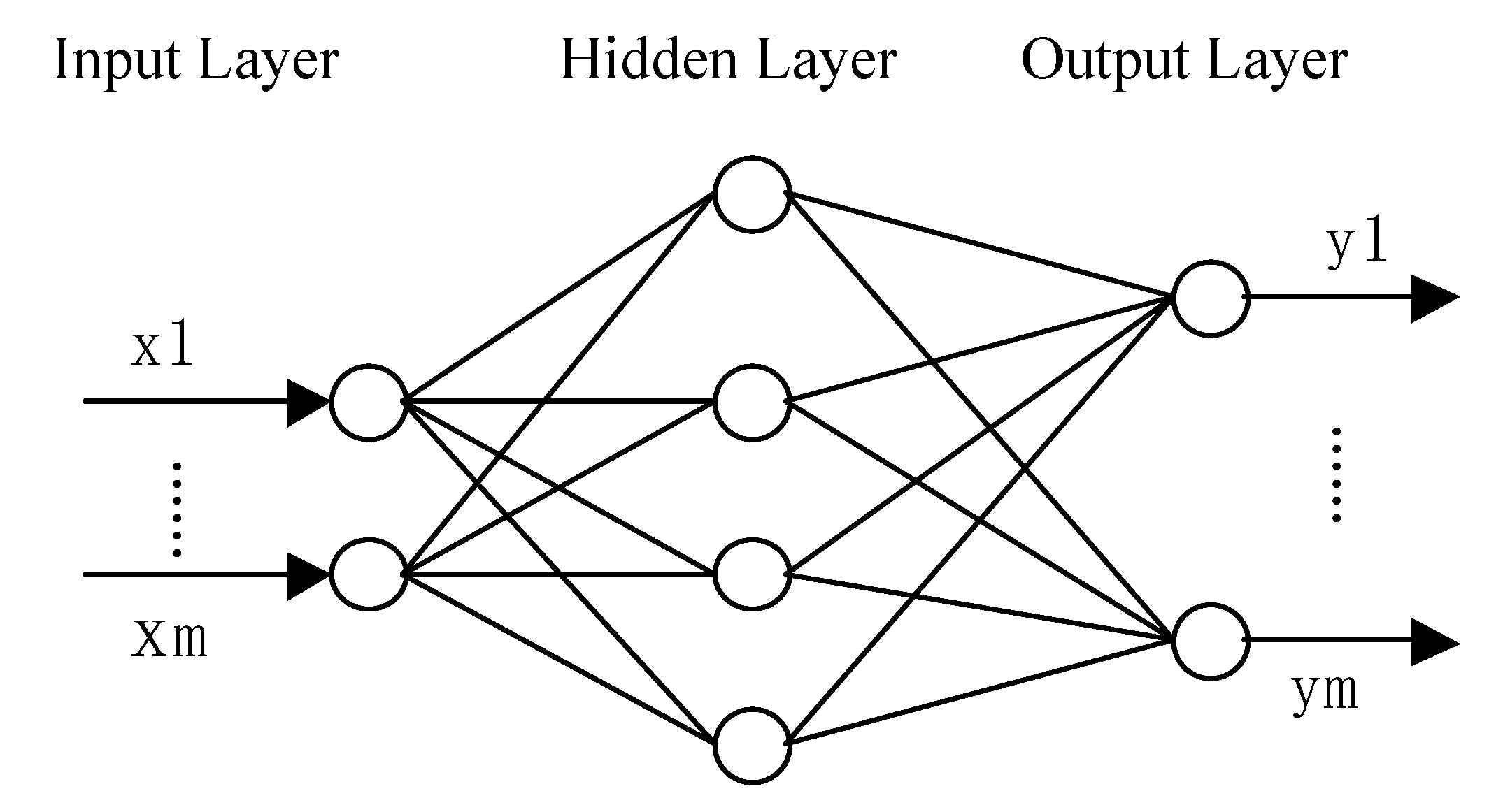
2.3. BP Neural Network Model

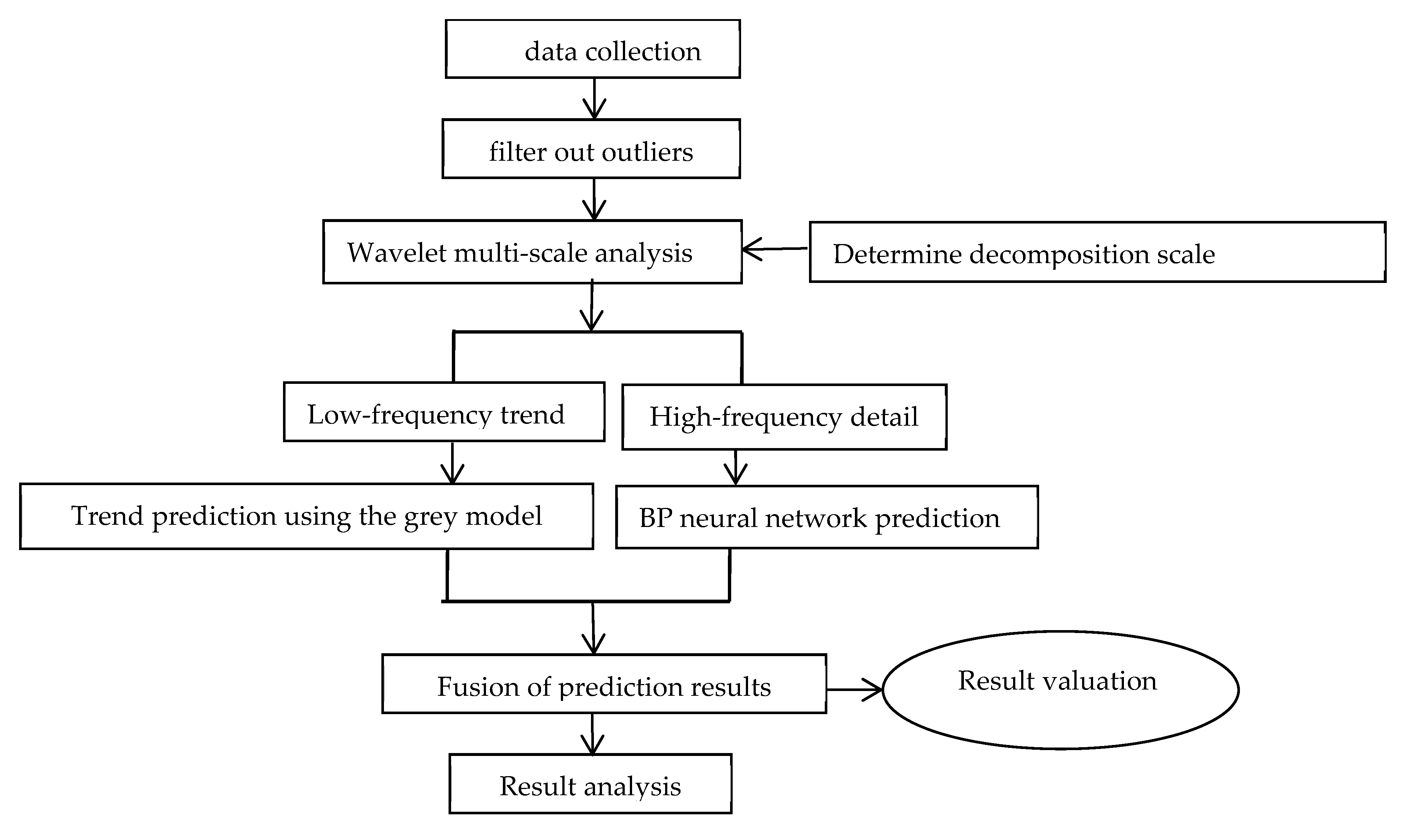
The BP (Back Propagation) neural network (BPNN) is based on the error backpropagation algorithm. Through multiple finite iterations, a multi-layer feedforward neural network that meets the training criteria is constructed [14]. Its typical structure includes a three-level information processing mechanism of an input layer, a hidden layer, and an output layer (Figure 1). The input layer receives the feature vector of the monitoring data, the hidden layer conducts nonlinear feature abstraction, and the output layer generates the target predicted value. In this study, the settlement monitoring data is divided into a training set and a test set, where the early observation data serves as the input layer, and the later predicted data serves as the output layer. The number of nodes in the hidden layer is calculated using the empirical formula [23], as shown in Equation (7):

$$\mathrm{h}=\sqrt{\mathrm{m}+\mathrm{n}}+\mathrm{a}$$

(7)

In the formula, $\mathrm{h}$ is the number of nodes in the hidden layer; $\mathrm{m}$ is the number of nodes in the input layer; $\mathrm{n}$ is the number of nodes in the output layer; and $\mathrm{a}$ is an adjustment constant ranging from 1 to 10.

2.4. Improved Model

Aiming at problems such as the coupling of multi-source interferences and significant non-stationary fluctuations in the health monitoring data of heritage structures, which lead to the low prediction accuracy of traditional GM(1,1) models [21], this study proposes a GM(1,1)-BP neural network fusion prediction model based on wavelet multi-scale decomposition. Through the construction of a technical path of “frequency domain decomposition-feature modeling-data fusion”, this model realizes the collaborative optimization of trend prediction and detail correction, and systematically improves the analysis ability of complex monitoring time-series. The modeling idea of the entire prediction model is as follows:

(1)

Time-frequency feature decoupling: The Mallat algorithm is used to perform wavelet decomposition on the original monitoring sequence [24]. By setting the optimal number of decomposition layers $\mathrm{n}$, the low-frequency approximate component $A_j$ representing the long-term trend and the high-frequency detail component $D_j$ containing the environmental disturbance features are obtained.

(2)

Trend extrapolation modeling: A GM(1,1) model is established for the low-frequency component and prediction is carried out. The equation is expressed as:

$${\displaystyle \frac{\mathrm{d}{X}^{(1)}}{d_t}}+a{X}^{(1)}=b$$

(8)

In the equation, the parameter $\mathrm{a}$ reflects the system development coefficient, and $\mathrm{b}$ is the grey action quantity.

(3)

Detail feature learning: An adaptive BP neural network is constructed for the high-frequency component $D_j$. The gradient descent algorithm is used to update the network weights. The hyperbolic tangent function is used in the hidden layer to enhance the nonlinear expression ability.

(4)

Dynamic fusion reconstruction: A fusion function that takes into account the trend information and detail information is established, and the time-domain reconstruction is realized through the inverse wavelet transform:

$$\widehat{Y}(t)={\widehat{Y}}_{GM}+{\widehat{Y}}_{BP}$$

(9)

The innovations of this study are as follows: Firstly, through wavelet decomposition, the limitation of the traditional model’s mixed processing of time-frequency features is broken through, and the effective decoupling of the monitoring signal in the scale space is achieved. Secondly, a complementary advantage mechanism between the grey model and the neural network is constructed. The GM(1,1) model captures the macroscopic trend changes, and the BP neural network model analyzes the microscopic fluctuation features. Figure 2 shows the flow chart of the experiment in this paper.

2.5. Model Accuracy Test

The accuracy evaluation grade of the model refers to the reference table for the accuracy test grade of the grey model proposed by Professor Deng Julong [22], which is used to evaluate the reliability of the model. The definition is based on the posterior variance test, and the model accuracy grade is mainly divided through two indicators: the posterior variance ratio $C$ and the probability of small error $P$.

Let $x$ be the original data sequence, $\overline{x}$ be the mean value of the original data sequence, $\widehat{x}$ be the corresponding predicted data sequence, n be the length of the original data sequence, $e$ be the residual sequence, $\overline{e}$ be the mean value of the residual sequence, $k$ be the k-th data in the original data sequence, $S_1$ be the standard deviation of the original data sequence, and $S_2$ be the standard deviation of the residual sequence.

Posterior variance ratio:

$$C:C=S_2/S_1$$

(10)

The calculation formula for the standard deviation $S_1$ of the original data sequence is:

$$S_1=\sqrt{{\displaystyle \frac{{\displaystyle \sum _{\mathrm{k}-1}^{\mathrm{n}}(x(k)-\overline{x}{)}^2}}{n-1}}}$$

(11)

The calculation formula for the standard deviation $S_2$ of the residual sequence is:

$$S_2=\sqrt{{\displaystyle \frac{{\displaystyle \sum _{\mathrm{k}-1}^{\mathrm{n}}(e(k)-\overline{e}{)}^2}}{n-1}}}$$

(12)

In the Formula (12), $e(k)=x(k)-\widehat{x}(k)$, $x(k)$ is the k-th data in the original data sequence, and $\widehat{x}(k)$ is the corresponding k-th predicted data.

Probability of small error:

$$P:P=P\left(\left|e(k)-\overline{e}\right|<0.6745S_1\right)$$

(13)

Through a large number of empirical analyses, the grade standards is shown in

Table 1. Reference Table for Accuracy Test Grades.

Grade	Posterior Variance Ratio C	Probability of Small Error p	Model Evaluation
First Grade	$C\le 0.35$	$P\ge 0.95$	Excellent (High Precision)
Second Grade	$0.35<C\le 0.50$	$0.80<P\le 0.95$	Good
Third Grade	$0.50<C\le 0.65$	$0.70<C\le 0.80$	Qualified
Fourth Grade	$C>0.65$	$P\le 0.7$	Unqualified

.

3. Experimental Results and Analysis

3.1. Overview of the Case

This study takes the Huang Rongyuan Hall, a historic and cultural building on Gulangyu Island, as the research object, and conducts deformation analysis and prediction research based on its settlement monitoring data. The building is located at No. 32 Fujian Road, Gulangyu Island (24°26′58″ N, 118°03′43″ E). It was initially built in 1920. Its architectural style integrates Western-style columns, Nanyang-style arcades, Chinese-style eaves, and modern structural technologies. It is a typical representative of the integration of diverse cultures in the early 20th century and was included in the “Gulangyu Island: Historic International Settlement” World Heritage List in 2017. In order to ensure the safety of the building, according to the “Code for Safety Monitoring of Cultural Relic Buildings” [25], and considering that the Huang Rongyuan Hall is a “classical masonry structure with multiple load-bearing columns”, a total of five high-precision settlement monitoring points are arranged in the Huang Rongyuan Hall (with a spacing of 8–12 m between the points) [26]. Four measuring points are set at the corners of the building to monitor the overall settlement trend. Given the importance of the load-bearing columns in supporting the weight of the building, a measuring point is set at the bottom of the giant column on the front facade of the building, that is, on the column foundation, to monitor the settlement of the giant column and the stability of the main structure, specifically referring to research on similar ancient buildings by Yuan Bao et al. [27].

High-precision electronic levels are used to achieve the real-time collection of settlement data. During the observation process, referring to the case of the Xiajia Culture Site at Erdaojingzi [26], if the cumulative settlement of the cultural relic building reaches 30 mm, it is considered an abnormal monitoring value, and it is necessary to immediately verify whether it is a real settlement. When the maximum settlement rate of the building is less than 0.01 mm/d to 0.04 mm/d, it can be considered that the stable state has been reached. Here, 15 periods of settlement monitoring data from 1 November to 31 November of the C1 deformation monitoring point with typical deformation characteristics were selected to verify the engineering applicability of the prediction model proposed in this paper.

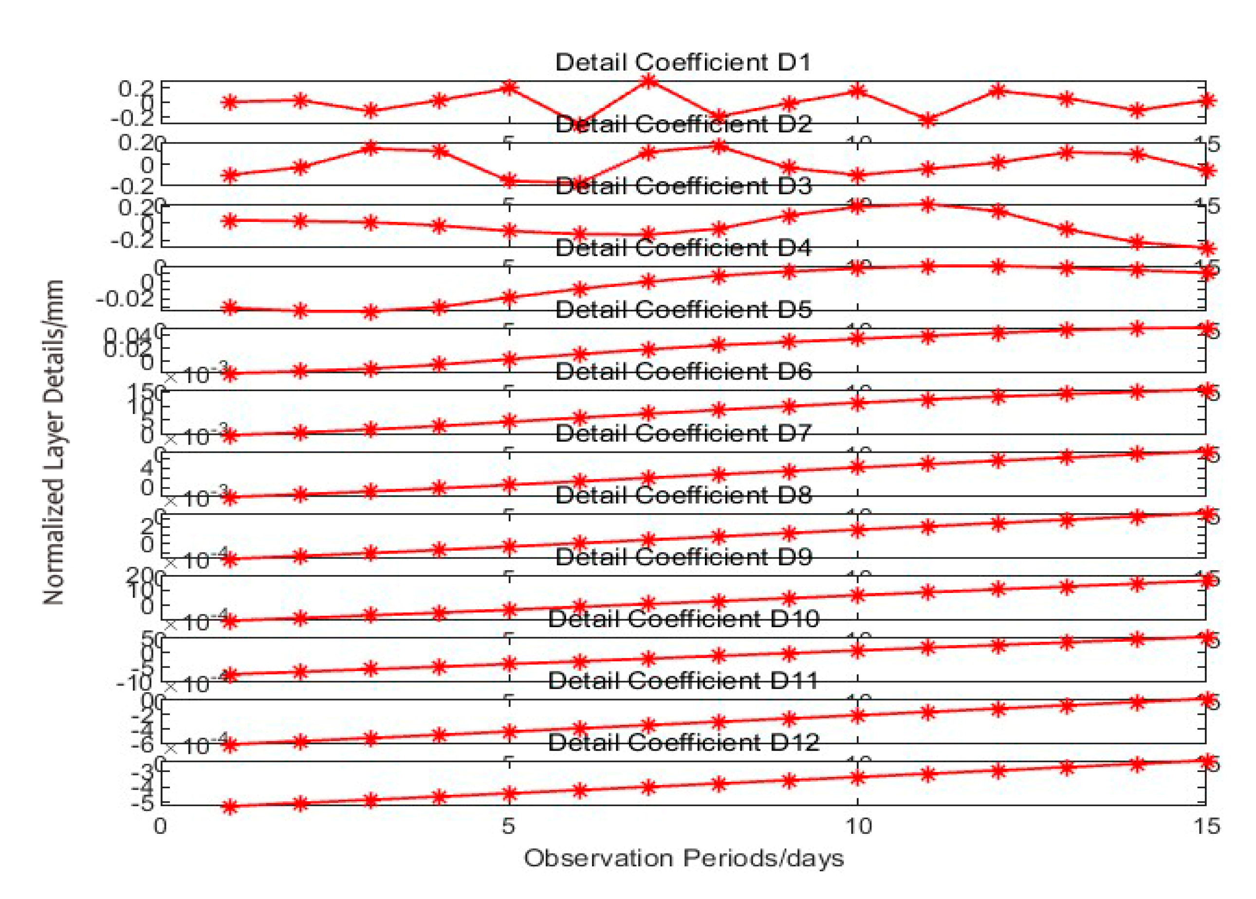
3.2. Data Processing Procedure

3.2.1. Data Preprocessing Process

In this study, by integrating wavelet multi-scale analysis with grey models and machine learning algorithms, the aim is to break through the limitations of traditional methods in non-stationary time-series prediction and verify the effectiveness of the proposed method. The settlement time-series data of the monitoring point of the Huang Rongyuan Hall on Gulangyu Island is taken as the object to carry out the verification of the prediction model. The settlement curve shown in Figure 3 exhibits significant non-stationary characteristics, and the cumulative settlement amount ranges from 6.4870 to 7.1220 m.

In wavelet multi-scale analysis, there are various choices for key parameters such as wavelet basis functions and decomposition levels, and these different choices will lead to certain differences in the prediction effect. In this paper, the point at which the change rate of the root mean square error (RMSE, hereinafter referred to as RMSE) between the original signal and the reconstructed signal after removing the high-frequency part tends to be stable [28] is used. That is, when the change rate of the RMSE tends to 1, the minimum wavelet decomposition layer number is initially screened out, and it can be considered that the high-frequency part and the low-frequency part are preliminarily and effectively separated. Then, by comparing the prediction performance of the models above the minimum decomposition layer number through experiments, the decomposition layer number is determined to be set as 12 layers. Due to its symmetry, compact support, noise robustness, and matching with structural signals, Sym5 is selected as the optimal wavelet basis function. Figure 4 shows the high-frequency detail components D1–D12 after multi-scale decomposition.

3.2.2. Processing Processes of the Grey Model and the BP Neural Network

The grey model is used to build a model for the low-frequency approximation component. During the modeling process, Min–Max normalization is adopted to map the data to the interval of [−1, 1]. A GM(1, 1) model is constructed for the low-frequency component, and the parameters of the grey differential equation, a = −0.0028 and b = 6.7618, are solved by the least squares method. Figure 5 shows the comparison results between the predicted values and the measured values. The average absolute error (MAE) of the predictions for the last five periods is 0.0296 mm, which verifies the model’s ability to capture the trend terms.

For the high-frequency detail component, a BP neural network is used for modeling. A deep structure with three hidden layers is constructed. The number of nodes in the input layer is set to four; the numbers of neurons in the hidden layers are 10, 8, and 5, successively; and the output layer is set with one node for outputting the predicted value of the settlement amount. During the training process, the maximum number of training times is set to 500 times to avoid the risk of overfitting. The initial value of the learning rate is set to 0.01, and the target error is set to 0.0001, which serves as one of the training termination conditions. The initial weights and thresholds are generated by random numbers within the interval of [−0.5, 0.5] to ensure that the initial state of the network has randomness and diversity. The settlement monitoring data is divided into a training set and a test set according to the ratio of 6:4. The Levenberg–Marquardt (LM) algorithm is adopted as the learning function for model training. This algorithm has the advantages of fast convergence speed and high stability in the processing of small-scale data. All model construction and experiments are completed based on the MATLAB R2024a platform, and its neural network toolbox and data processing functions are used to realize the development and verification of the algorithm. Figure 6 shows the comparison between the predicted values and the true values of the high-frequency details. The root mean square error (RMSE) is 0.1348 mm, and the error between peaks is controlled within ±0.6 mm. The deformation detection values obtained through the model have a high degree of consistency with the actual values, which verifies the applicability of the model.

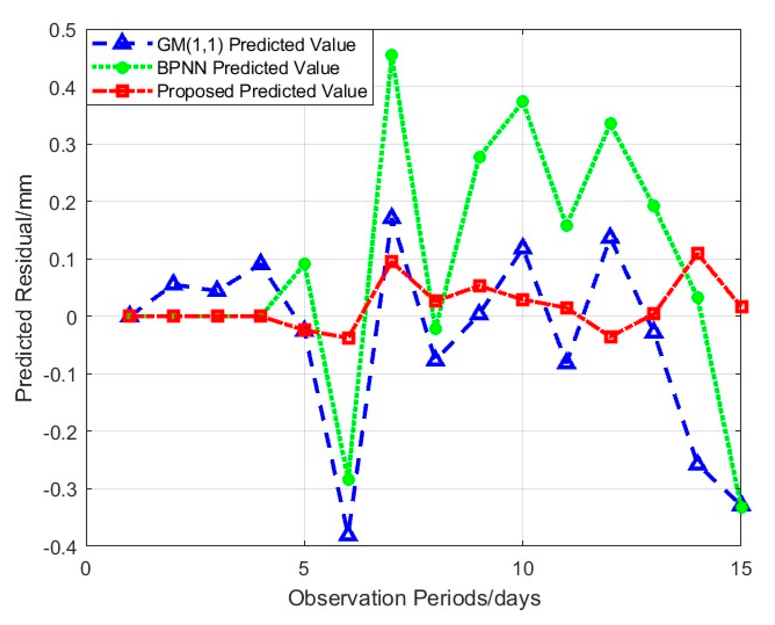
3.3. Results Analysis

Based on the above analysis, in this study, the prediction results of the grey model for the low-frequency trend and the prediction results of the neural network for the detailed information are combined through the inverse wavelet transform [16] to obtain the final deformation prediction results, as shown in Figure 7 and Figure 8. During the wavelet reconstruction process, the synchronization of the prediction results of the two channels in the time-frequency space is achieved through the following mechanisms: First, by utilizing the multi-scale decomposition characteristics of the wavelet transform, during the decomposition process, the prediction sequences of the grey model and the neural network are subjected to wavelet decomposition at the same scale to ensure that the coefficients of the two in each frequency band (such as the low-frequency trend term and the high-frequency fluctuation term) strictly correspond to each other. Second, during the inverse transform process, strictly following the principle of the linear superposition of wavelet reconstruction, a unified reconstruction operation is performed on the fused coefficients. Through this process, the time-frequency information of the low-frequency and high-frequency components is superimposed in the time domain according to the mathematical relationship of the wavelet transform, ensuring that the final prediction result not only retains the advantageous information of the two channels, but also satisfies the continuity and consistency in the physical space.

Figure 7 and Figure 8 qualitatively compare the fitting and prediction results of the model in this paper.

Table 2. Comparative analysis of fitting and predictive performance across three models (unit: mm).

Models	RMSE	MAE	Maximum Positive Residual	Maximum Negative Residual	Peak-to-Peak Value of the Residual
GM(1,1)	0.1651	0.12	0.1708	−0.3808	0.5516
BPNN	0.2305	0.17	0.4540	−0.3327	0.7867
Improved model	0.0440	0.0296	0.1093	−0.0373	0.1466

shows a quantitative comparison of the fitting and prediction results of the three models. In terms of the trend fitting ability, due to the constraints of the linear assumption, the peak-to-peak value of the residuals of the GM(1,1) model reaches 0.5516 mm, and it cannot reflect the non-linear dynamics of the actual settlement. In terms of the detail analysis ability, although the BP neural network can capture high-frequency fluctuations, the lack of trend constraints leads to an overall deviation (the deviation of the trend term is as high as 0.45 mm). According to the analysis of the residual curve in Figure 8, it can be observed that the absolute values of the maximum residuals of the other two models during prediction both exceeded 0.2 mm. The residual curve in Figure 8 and the results in Table 2 show that the residuals of the GM(1,1) model exhibit significant temporal correlation and that there is a systematic bias. The residual in the 12th period reaches −0.3808 mm, which reflects the insufficient adaptability of the linear model to the stage of accelerated settlement. The BP neural network model has multiple overshoot phenomena (the residual in the 14th period is +0.454 mm), indicating that the generalization ability of the network to sudden environmental disturbances is limited. However, the stability of the residual sequence of the model in this paper verifies the random nature of the model error. The improved model in this paper is significantly superior to the GM(1,1) model and the BP neural network model in both deformation trend fitting and detail feature capture.

Table 3. Comparative analysis of the predicted results across the three models (unit: mm).

	Settlement Value	GM (1,1)	BPNN	Improved Model
Number of Prediction Periods		Predicted Value	Predicted Value	Predicted Value
The 11th period	6.823	6.9655	6.7264	6.8691
The 12th period	6.92	6.9853	6.7869	7.1573
The 13th period	6.854	7.0050	6.7855	6.9731
The 14th period	6.846	7.0249	6.7341	6.6577
The 15th period	6.794	7.0447	7.04870	6.6999
RMSE		0.1651	0.2305	0.0440
MAE		0.1200	0.1700	0.0296

shows the evaluation results of the prediction accuracy for the 11th to 15th periods. As can be seen from Table 2, the RMSE of the GM(1,1) model is 0.1651 mm, the RMSE of the BP neural network model is 0.2305 mm, and the RMSE of the method proposed in this paper is 0.0440 mm. Compared with the traditional grey model, the improvement rate of the method in this paper is as high as 73.35%. The improvement rate of the MAE of the method in this paper is 75.33% compared with that of the traditional grey model. The method proposed in this paper is superior to the traditional GM(1,1) model and the BP model.

Next, the posterior variance ratio test method is used to evaluate the accuracy of the improved model in this paper, the GM(1,1) grey model, and the BP neural network model. The first-level accuracy requires that C ≤ 0.35 and p ≥ 0.95; the second level requires that C ≤ 0.5 and p ≥ 0.80; the third level requires that C ≤ 0.65 and p ≥ 0.70; and the fourth level means that C > 0.65 or p < 0.70. The posterior variance ratio C, the probability of small error p, and the comprehensive accuracy grade of each model are shown in

Table 4. Posterior Difference Test (C and p Values) for Three Prediction Models.

Models	Accuracy Level	Posterior Variance Ratio C	Probability of Small Error p
GM(1,1)	The fourth level	1.0592	0.5333
BPNN	The fourth level	1.4113	0.4667
Improved model	The first level	0.2681	1

. According to the data in Table 4, the accuracy grades of the grey model and the neural network are at the fourth level. However, by introducing the BP neural network to improve the model in this paper, the accuracy reaches the first level, significantly improving the prediction accuracy.

The experimental findings demonstrate that the prediction accuracy of the proposed model has been augmented by over 70% in comparison with a solitary model. Notably, the root-mean-square error has been diminished to 0.044 mm. This substantial improvement markedly bolsters the stability and generalization capacity of the prediction outcomes. The method presented herein transcends the limitations of traditional models in representing the characteristics of nonlinear time series. It further furnishes a spatiotemporally adaptable assessment instrument for the early warning of the structural health condition of heritage structures. Evidently, the prediction performance of this method is conspicuously superior to that of a single model.

4. Conclusions

In view of the limitations of the grey system model in settlement prediction, such as its stringent requirements for data stability, high sensitivity to data fluctuations, and relatively low prediction accuracy, a novel prediction model integrating the GM(1,1) model and the BPNN model, based on wavelet transform, was proposed. By employing the settlement monitoring data of heritage structures, the GM(1,1) model, the BPNN model, and the method developed in this study were utilized for prediction analysis, respectively. The following conclusions were derived:

(1)

Substantial Enhancement in Model Performance

The mean absolute errors (MAEs) of the GM(1,1) model, the BP model, and the improved model presented herein are 0.12 mm, 0.17 mm, and 0.03 mm, respectively. The root mean square errors (RMSEs) are 0.17 mm, 0.23 mm, and 0.04 mm, respectively. In comparison with the GM(1,1) model and the BP neural network model, the improvement rates of the MAE of the fusion model reach 75% and 82.4%, respectively, and those of the RMSE are 76.5% and 82.6%, respectively. These quantitative results unequivocally validate the significant superiority of the fusion model in terms of prediction accuracy. The coefficient of determination (R²) between the prediction results of this model and the measured values is above 0.87, and the RMSE = 0.04 < 0.1 mm. Evidently, this model can offer reliable technical support for structural safety early warnings and preventive protection measures.

(2)

Multi-scale Synergistic Mechanism

Through wavelet decomposition, the deformation monitoring signal is effectively decoupled into low-frequency trend components and high-frequency detail components. Leveraging the extrapolation advantage of the GM(1,1) model and the nonlinear fitting capabilities of the BP neural network for feature modeling, the collaborative optimization of “macro-trend grasping-micro-fluctuation analysis” is achieved. As a result, the derived deformation trend is much closer to the actual deformation scenario, which is of great significance for the safe operation of heritage structures.

(3)

Deficiencies and Improvement Directions

The wavelet-grey-BP neural network fusion model has the following deficiencies and requires further improvement. Settlement prediction methods based on single deep learning models demonstrate powerful feature extraction capabilities in scenarios with sufficient data. In contrast, this fusion model focuses more on addressing the practical challenges of scarce and highly non-stationary settlement data on ancient buildings. Although the effectiveness of the fusion model has been verified, deep learning models still possess significant advantages. In the follow-up to this work, exploring ways of combining the fusion model with other cutting-edge algorithms should be considered. In addition, the parameter settings of the wavelet transform, as well as the combination of the grey model and the BP neural network, still mainly rely on experience and the trial-and-error method. Compared with the research on adaptive weight adjustment, a complete set of adaptive parameter optimization mechanisms has not been formed yet, which to a certain extent, limits the further improvement of the model’s performance.

References

1. Hou, J.; Zhou, J.; He, Y.; Hou, B.; Li, J. Automatic reconstruction of semantic façade model of architectural heritage. Heritage Sci. 2024, 12, 400. [Google Scholar] [CrossRef]
2. Delcea, C.; Javed, S.A.; Florescu, M.-S.; Ioanas, C.; Cotfas, L.-A. 35 years of grey system theory in economics and education. Kybernetes 2025, 54, 649–683. [Google Scholar] [CrossRef]
3. Jiang, J.; Liu, C.; Yao, Y.; Lu, Y.; Xie, W.; Liu, C.; Li, Q. An Improved Grey Model with Time Power and Its Application. Complexity 2022, 2022, 6910865. [Google Scholar] [CrossRef]
4. Huang, C.; Cao, Y.; Zhou, L. Application of optimized GM (1,1) model based on EMD in landslide deformation prediction. Comput. Appl. Math. 2021, 40, 261. [Google Scholar] [CrossRef]
5. Kankanamge, Y.; Hu, Y.; Shao, X. Application of wavelet transform in structural health monitoring. Earthq. Eng. Eng. Vib. 2020, 19, 515–532. [Google Scholar] [CrossRef]
6. Comert, G.; Begashaw, N.; Medhin, N.G. Bayesian parameter estimations for grey system models in online traffic speed predictions. arXiv 2021. [Google Scholar] [CrossRef]
7. Wang, X.; Li, W.; Ma, M.; Yang, F.; Song, S. Bridge damage identification based on encoded images and convolutional neural network. Buildings 2024, 14, 3104. [Google Scholar] [CrossRef]
8. Yun, D.Y.; Shim, H.B.; Park, H.S. SSI-LSTM network for adaptive operational modal analysis of building structures. Mech. Syst. Signal Process. 2023, 195, 110306. [Google Scholar] [CrossRef]
9. Yessoufou, F.; Zhu, J. Classification and regression-based convolutional neural network and long short-term memory configuration for bridge damage identification using long-term monitoring vibration data. Struct. Health Monit. 2023, 22, 4027–4054. [Google Scholar] [CrossRef]
10. Chaiyasarn, K. Crack detection in historical structures based on convolutional neural network. Int. J. Geomate 2018, 15, 240–251. [Google Scholar] [CrossRef]
11. Xiao, F.; Yan, Y.; Meng, X.; Xu, L.; Chen, G.S. Parameter identification of beam bridges based on stiffness separation method. Structures 2024, 67, 107001. [Google Scholar] [CrossRef]
12. Li, Z.; Li, D.; Shen, W. Methods for Visualizing Deep Learning to Elucidate Contributions of Various Signal Features in Structural Health Monitoring. J. Comput. Civ. Eng. 2025, 39, 04025042. [Google Scholar] [CrossRef]
13. Sun, X.; Xin, Y.; Wang, Z.; Yuan, M.; Chen, H. Damage detection of steel truss bridges based on gaussian bayesian networks. Buildings 2022, 12, 1463. [Google Scholar] [CrossRef]
14. Saadatmorad, M.; Jafari-Talookolaei, R.-A.; Khatir, S.; Fantuzzi, N.; Cuong-Le, T. Frugal wavelet transform for damage detection of laminated composite beams. Comput. Struct. 2025, 314, 107765. [Google Scholar] [CrossRef]
15. Mousavi, V.; Rashidi, M.; Ghazimoghadam, S.; Mohammadi, M.; Samali, B.; Devitt, J. Transformer-based time-series GAN for data augmentation in bridge digital twins. Autom. Constr. 2025, 175, 106208. [Google Scholar] [CrossRef]
16. Mallat, S. A Wavelet Tour of Signal Processing. The Sparse Way, 3rd ed.; Elsevier: Amsterdam, The Netherlands; Academic Press: Cambridge, MA, USA, 2009. [Google Scholar] [CrossRef]
17. Ma, Q.; Xu, J.; Gao, X.; Liu, M. Structural damage localization based on wavelet packet analysis under varying environment effects. J. Civ. Struct. Health Monit. 2025, 1–21. [Google Scholar] [CrossRef]
18. Li, Q.; Xie, J. Bridge Alignment Prediction Based on Combination of Grey Model and BP Neural Network. Appl. Sci. 2024, 14, 7955. [Google Scholar] [CrossRef]
19. Hao, W.; Yin, H.; Liu, J.; Ma, R.; Zhao, D.; Lu, S. Seismic response prediction of soil tunnel structure based on CNN-LSTM model. Structures 2025, 73, 108381. [Google Scholar] [CrossRef]
20. Dejamkhooy, A.; Dastfan, A.; Ahmadyfard, A. Modeling and Forecasting Nonstationary Voltage Fluctuation Based on Grey System Theory. IEEE Trans. Power Deliv. 2017, 32, 1212–1219. [Google Scholar] [CrossRef]
21. Xiao, Y.T.; Fan, S.J.; Zang, J.F.; Mu, C.L.; Diao, J. Application research on improved GM(1,1) model in foundation pit settlement prediction of urban rail transit engineering. Geomat. Eng. 2024, 33, 62–67. [Google Scholar]
22. Deng, J. Grey System Theory Tutorial; Huazhong University of Science and Technology Press: Wuhan, China, 2013. [Google Scholar]
23. Wilamowski, B.M.; Yu, H. Neural network learning without backpropagation. IEEE Trans. Neural Netw. 2010, 21, 1793–1803. [Google Scholar] [CrossRef] [PubMed]
24. Yu, T.; Hu, W.S.; Wu, J.; Li, H.F.; Qiao, Y. Extracting vibration information of Runyang Bridge based on wavelet threshold denoising and EMD decomposition method. J. Vib. Shock. 2019, 38, 264–270. [Google Scholar]
25. DB11/T 1473—2017; Code for Safety Monitoring of Cultural Relic Buildings [Local Standard]. Beijing Municipal Bureau of Cultural Heritage: Beijing, China, 2017.
26. Chen, J. Exploration of Settlement Observation and Analysis Methods for Cultural Relic Buildings. Henan Build. Mater. 2020, 3–4. [Google Scholar]
27. Yuan, B. Deformation monitoring analysis method of ancient buildings. Geomat. Technol. Equip. 2023, 25, 1–5. [Google Scholar]
28. He, Y.; Jin, P.; Jiang, C. An airborne dual PolInSAR orbit error removal method based on multi-scale correlation analysis. J. Geo-Inf. Sci. 2021, 23, 670–679. [Google Scholar] [CrossRef]
Figure 1. Schematic Diagram of the Structure of the Feedforward Neural Network.
Buildings 15 02240 g001
Figure 2. Experimental flow chart of this paper.
Buildings 15 02240 g002
Figure 3. Deformation Diagram of Monitoring Points.
Buildings 15 02240 g003
Figure 4. Low-frequency and high-frequency parts.
Buildings 15 02240 g004
Figure 5. Low-frequency prediction results.
Buildings 15 02240 g005
Figure 6. High-frequency prediction results.
Buildings 15 02240 g006
Figure 7. Results comparison of the three models.
Buildings 15 02240 g007
Figure 8. Comparison of the residual of the three models.
Buildings 15 02240 g008