Fatigue Damage Prognosis Method for Main Girders of Cable-Stayed Bridges Based on Wavelet Neural Network

Abstract

At present, the research on bridge structure health monitoring mainly focuses on discovering existing structural damage and less on predicting when the damage will occur in the future. This paper proposes a fatigue damage prognosis method for the main girders of cable-stayed bridges based on wavelet neural networks (WNNs). This method integrates WNN with multi-scale finite element modeling to predict fatigue damage progression. First, the theoretical foundation and implementation algorithms of the WNN are elaborated on and applied to forecast the future load environments of cable-stayed bridges. Subsequently, multi-scale finite element models are employed to derive stress influence lines for critical fatigue-prone regions in the main girder of the cable-stayed bridge. Finally, fatigue reliability methods are utilized to predict the fatigue reliability indices, service life, and failure probabilities of critical fatigue details. The proposed prognosis method in this paper can accurately predict the future operation conditions and remaining service life of bridge structures so as to provide a more reasonable maintenance strategy for bridge structures.

1. Introduction

At present, structural health monitoring (SHM) systems, with the goal of ensuring bridge operational safety, have been widely applied to the operational monitoring of long-span bridges [1,2,3]. In order to achieve the best monitoring effect, many engineers have optimized the sensor type, number, location, and data transmission and storage and analysis technology [4,5]. The primary purpose of SHM is to evaluate the operational status of the main bridge structure using data acquired by its sensors. Damage identification can infer structural physical parameters (e.g., mass, stiffness, and damping) through static/dynamic structural responses (e.g., displacement, velocity, frequency, mode shapes, and energy). This process is typically divided into four levels: (1) determining whether damage has occurred; (2) identifying the specific location of structural damage; (3) assessing the extent of structural damage; and (4) evaluating the impact of structural damage on structural performance and load-bearing capacity. However, under current technological and practical conditions, identifying early-stage structural damage remains challenging. In this context, prognosis technology may be an effective method to overcome the bottlenecks in SHM systems.

Prognosis is endowed with distinct meanings across different fields. In the medical field, injury/disease prognosis addresses the following: (1) What symptoms precede the onset of illness? (2) What effects will a treatment produce after diagnosis? (3) What post-recovery measures can prevent relapse? Subsequently, the engineering community has recognized the significant value of prognosis. For example, in military applications, damage prognosis answers the following questions: (1) Can combat-damaged aircraft or naval vessels continue fighting? (2) Can they return to base, or should they be abandoned? In aerospace, damage prognosis quantifies the remaining useful life (RUL) of system components. In mechanical manufacturing, it determines when to perform maintenance to minimize downtime while avoiding fatigue failure. In civil engineering, prognosis attempts to address the following: (1) When and where is structural damage likely to occur? (2) Can a damaged structure continue functioning effectively under complex service conditions (e.g., overload, earthquakes, typhoons, corrosion, or fatigue)? For instance, can a bridge withstand aftershocks after a major earthquake? (3) How do post-damage repair and maintenance strategies affect structural performance, thereby determining the optimal maintenance plan? These questions represent the major challenges hindering the development of bridge structural health monitoring systems [6,7,8].

Farrar and Lieven [2], Inman and Farrar [3], and Farrar and Hemez [6] have proposed that damage prognosis is the future theme of structural health monitoring (SHM), and damage prognosis is defined as follows: “Based on SHM systems, under the premise of understanding damage evolution mechanisms, combined with the service history and current condition of structures, to evaluate the current damage state of structures (first level), predict the future loading environment and structural performance (second level), and predict the remaining service life of structures through numerical simulation techniques and historical experience (third level)” [9], that is, the extent to which structural materials, geometric dimensions, boundary conditions, and changes in connections between structures affect current and future performance of structures. For example, a crack generated in a structure will affect its stiffness and geometric configuration. Depending on the crack size, location, and environmental conditions, this damage may negatively impact the structure immediately or may affect the overall structural performance after a period of development [10]. Damage prognosis is used to monitor and predict such a “process” to facilitate owners in making optimal decisions for bridge maintenance. Therefore, prognosis refers to predicting and preventing structural damage or degradation before structural failure occurs [11].

Currently, research on structural damage prognosis mainly focuses on fatigue damage prognosis. The implementation methods are divided into two categories: model-based damage prognosis [12,13,14,15,16,17] and data-driven damage prognosis [11,18,19,20,21,22]. These two approaches start from different perspectives but have no absolute boundaries. Physics-based damage prognosis methods can holistically understand monitored structures and effectively perform predictions; however, their computational load and data storage requirements are large, making real-time prediction almost impossible. Data-driven damage prognosis methods can establish learning models based on measured data, mainly including artificial neural network-based prognosis methods, fuzzy theory-based prognosis methods, reliability-based prognosis methods, and probability-based prognosis methods. Among these, wavelet neural network methods combine the noise reduction capability of wavelet analysis with the prediction abilities of neural networks, enabling faster convergence in iterative computations with high accuracy [18].

Based on the wavelet neural network method, combined with the multi-scale finite element model, the fatigue damage prognosis of the main girders of cable-stayed bridges is studied in this paper. Firstly, the theoretical basis and implementation algorithm of a wavelet neural network are described, and this network is applied to the prediction of the future load environment of cable-stayed bridge; then, combined with the multi-scale finite element model, the stress influence lines of the key parts of the main girder of a cable-stayed bridge are obtained; finally, the fatigue reliability, fatigue life, and failure probability of the key fatigue parts of the main beam are predicted by using the fatigue reliability method.

2. Damage Prognosis Method Based on Wavelet Neural Network

Many problems in civil engineering are nonlinear problems, and the relationship between variables is complex, so it is difficult to describe such engineering problems with exact mathematical or mechanical theory. As an artificial intelligence method, a wavelet neural network aims to establish the mathematical relationship between dependent variables and independent variables through limited self-learning. In essence, it is a self-learning network formed by simulating the working principle of neurons when people are thinking. Because of its learning ability, it can continuously adjust the weight of the network according to the set mode and input samples so that it has the abilities of function approximation and information processing [23].

Figure 1 is the most representative multi-input single-output wavelet neural network model. The input layer of the model has n nodes, the hidden layer has l nodes, the output layer is 1, and the network topology is n-l-1. The mathematical relationship between input and output can be established as

$$y={\displaystyle \sum _{k=1}^l{\nu }_k}{\psi }_k={\displaystyle \sum _{k=1}^l{\nu }_k}\psi ({\displaystyle \frac{{\displaystyle \sum _{i=1}^n{w}_{ki}}{\mathrm{x}}_i{-\mathrm{b}}_k}{a_k}})$$

(1)

where ${\mathrm{x}}_i$ is the wavelet neural network input value; $w_{ki}$ is the connection weight function of the k-th neuron in the hidden layer and the i-th cell in the input layer; ${\nu }_k$ is the connection weight between the k-th neuron of the hidden layer and the unit of the output layer; $\psi (\cdot )$ is wavelet neuron excitation function; $a_k$ and ${\mathrm{b}}_k$ are the expansion and translation parameters; and $y$ is the network output.

In the strict sense, a wavelet neural network approximates functions through some form of wavelet combination, in which $a_k$, ${\mathrm{b}}_k$, $w_{ki}$, and ${\nu }_k$ are determined by the network training.

The basic idea of the learning algorithm of a wavelet neural network is as follows. Based on an input and output sample library, the correlation weight function and the expansion and translation parameters are determined using the function fitting method so as to establish the mapping relationship between the input and output. The following is a widely used iterative algorithm based on gradient descent.

Given s learning samples ($x_{1s},x_{2s},\cdot \cdot \cdot ,x_{ns},d_s$), where s = 1, 2, …, S, the first subscript represents the input value vector component sequence number, and the second subscript represents the learning sample sequence number; $d_s$ is the network’s expected output corresponding to the input $(x_{1s},x_{2s},\cdot \cdot \cdot ,x_{ns})$. Setting $y_s$ as the actual output of the network corresponding to the input $(x_{1s},x_{2s},\cdot \cdot \cdot ,x_{ns})$, the error function, E, of the wavelet neural network can be defined as

$$E={\displaystyle \frac{1}{2}}{\displaystyle \sum _{s=1}^S{{(\mathrm{y}}_s-{\mathrm{d}}_s)}^2}={\displaystyle \frac{1}{2}}{\displaystyle \sum _{s=1}^S({\displaystyle \sum _{k=1}^l{\nu }_k}\psi (\frac{{\displaystyle \sum _{i=1}^n{w}_{ki}}{\mathrm{x}}_{is}-{\mathrm{b}}_k}{a_k})-d_s{)}^2}$$

(2)

The training principle of the wavelet neural network is to minimize the error function, $E$, by adjusting the relevant parameters of the network so that the output function, $y_s$, obtained by fitting can be used as the mapping function of the input and output.

It can be seen from Equations (1) and (2) that in order to obtain the optimal wavelet neural network, the network parameters $w_{ki}, {\nu }_k, a_k, {\mathrm{b}}_k$ need to be solved, which can be calculated by the following formula:

$$\left\{\begin{array}{l}{w}_{ki}=w_{ki}+\alpha ∆w_{ki}...............i=1,2,....,n;k=1,2,...,l\\ {\nu }_k={\nu }_k+\beta ∆{\nu }_k...................k=1,2,...,l\\ a_k=a_k+\gamma ∆a_k...................k=1,2,...,l\\ b_k=b_k+\eta ∆b_k...................k=1,2,...,l\end{array}\right.$$

(3)

where $\alpha , \beta , \gamma , \eta$ are learning rates.

For simplicity,

$$\mathrm{u}={\displaystyle \frac{{\displaystyle \sum _{i=1}^n{w}_{ki}}{\mathrm{x}}_{is}-{\mathrm{b}}_k}{a_k}}$$

(4)

$$\left\{\begin{array}{l}∆w_{ki}={\displaystyle \frac{\partial E}{\partial w_{ki}}}=(\mathrm{y}-\mathrm{d}\left)\right({\displaystyle \sum _{k=1}^l{\nu }_k{\psi }^{\prime }\left(\mathrm{u}\right)}){\displaystyle \frac{x_{is}}{a_k}}\\ ∆{\nu }_k={\displaystyle \frac{\partial E}{\partial {\nu }_k}}=(\mathrm{y}-\mathrm{d}\left)\right({\displaystyle \sum _{k=1}^l\psi \left(\mathrm{u}\right)})\\ ∆a_k={\displaystyle \frac{\partial E}{\partial a_k}}=(\mathrm{y}-\mathrm{d}\left)\right({\displaystyle \sum _{k=1}^l{\nu }_k{\psi }^{\prime }\left(\mathrm{u}\right)}\left)\right(-{\displaystyle \frac{u}{a_{\mathrm{k}}}})\\ ∆b_k={\displaystyle \frac{\partial E}{\partial b_k}}=(\mathrm{y}-\mathrm{d}\left)\right({\displaystyle \sum _{k=1}^l{\nu }_k{\psi }^{\prime }\left(\mathrm{u}\right)}){\displaystyle \frac{-1}{a_{\mathrm{k}}}}\end{array}\right.$$

(5)

where ${\psi }^{\prime }\left(\mathrm{u}\right)$ is the reciprocal of the first order of $\psi \left(\mathrm{u}\right)$. Substituting Equation (5) into Equation (3) can obtain the calculation error, E, relative error ratio, and new network parameters. Through iterative calculation, when the obtained relative error ratio meets the requirements, the output network parameters are the optimal solution.

At present, a variety of wavelet functions have been constructed, such as the Harr wavelet, the Meyer wavelet, the Daubechies wavelet, the Morlet wavelet, and the spline wavelet. Because the selection of the wavelet function has great flexibility, there is no unified standard as long as the allowable conditions are met. Among them, the Morlet wavelet is a Gaussian wave with finite support, symmetry, and cosine modulation and is most widely used in various fields. In this section, the Morlet wavelet basis function is selected as the excitation function of the wavelet neural network. There is no theoretical guidance for the selection of the number of neurons in the hidden layer. The main methods used are the experimental method and empirical formula method, in which the empirical formula includes the following [24]:

$$l=\sqrt{m\times n}$$

(6)

$$l=\sqrt{m+n}+t$$

(7)

$$l=\sqrt{0.43mn+0.12n^2+2.54\mathrm{m}+0.77n+0.35}+0.51$$

(8)

$$l={\displaystyle \frac{mn+\frac{1}{2}n(n^2+n)-1}{m+n}}$$

(9)

where n is the number of input nodes, m is the number of output nodes, $l$ is the number of hidden layer nodes, and $t$ is a constant between 1 and 20.

Theoretically, for a specific application problem, there should be an optimal number of hidden layer neurons. When the number of neurons in the hidden layer is selected by the experimental method, there is a certain blindness in determining the initial value of the number of neurons in the hidden layer, and it is difficult to ensure the rationality of the number of neurons. The number of neurons in the hidden layer calculated according to the empirical formula is often only the approximate range of obtaining the optimal number of neurons in the hidden layer, and the empirical formula used is summarized based on experiments in other fields, which is not necessarily suitable for any model constructed. Therefore, the empirical formula can only be used as a reference to determine the number of neurons in the hidden layer.

Let the number of hidden layer nodes of the three-layer wavelet neural network be l, and the number of input layer nodes is $n$; $w_{ki}$ is the connection weight from the k-th neuron in the hidden layer to the i-th neuron in the input layer, and ${\nu }_k$ is the connection weight between the k-th neuron in the hidden layer and the unit in the output layer. The setting of peer-to-peer initialization parameters $w_{ki}, {\nu }_k, a_k, {\mathrm{b}}_k$ can obtain empirical initial parameters through signal analysis and processing. A reasonable parameter setting can reduce the number of iterations and increase efficiency. However, the empirical formula has not been verified by a wide range of data. Compared with the cyclic ordered signals in the field of mechanical engineering, the measured signals in the field of civil engineering are more discrete and random, so the discussion of the initial parameters of the two cannot be generalized. The author has tried to use the empirical formula from the field of machinery to set the initial parameters, and the effect is not significant. When the more primitive random matrix conforming to the standard normal distribution is used as the initial parameter, the accuracy and efficiency meet the requirements.

3. Prediction of Future Vehicle Load Model for Cable Stayed Bridge

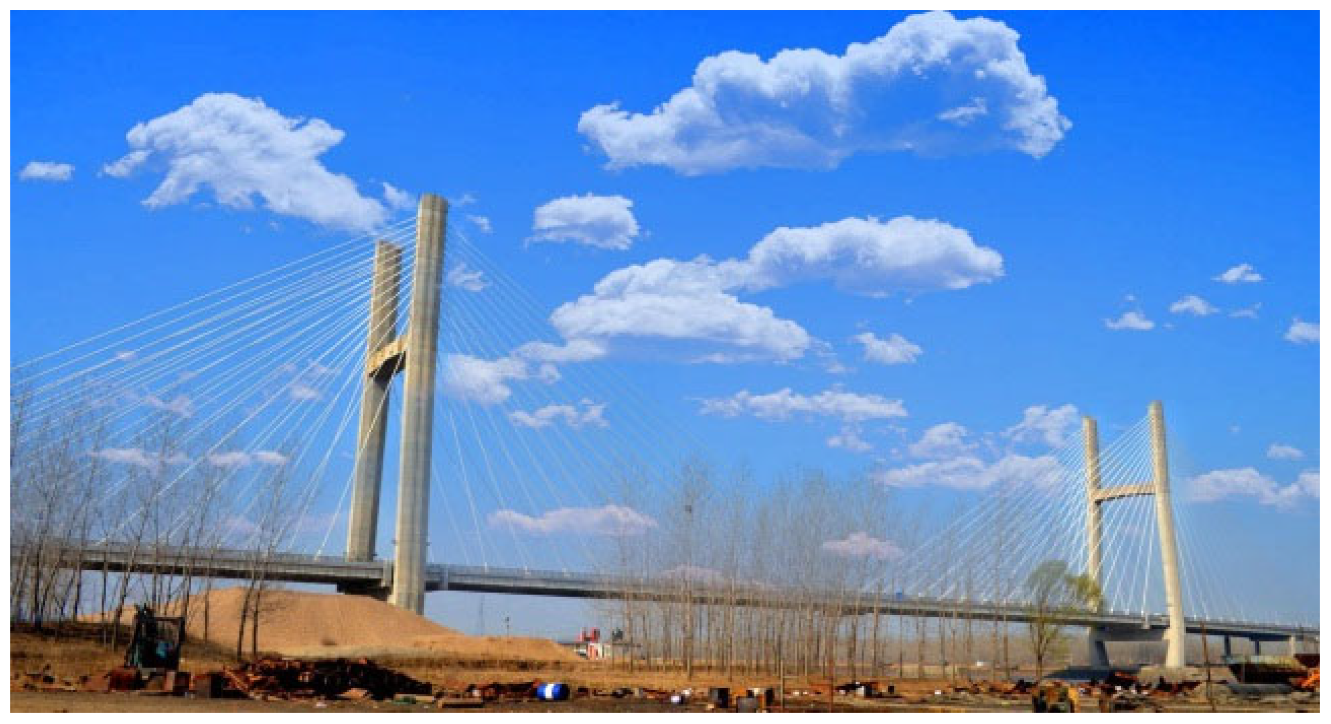
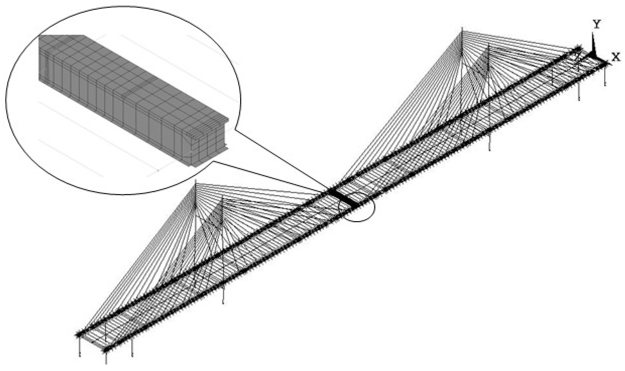
This study takes a cable-stayed bridge project as the research object. The total length of the bridge is 640 m, and the symmetrical layout of the main span is 340 m (see Figure 2 for the structural diagram). The main structural features of the bridge are as follows: (1) the bridge tower adopts a reinforced concrete structure, with a total height of 121 m; (2) the main beam adopts a steel–concrete composite beam system; (3) the bridge deck system is a prestressed concrete structure with a design width of 34 m and a section height of 3.08 m. The bridge project was completed and opened to traffic in May 2006 and has been in operation for 19 years.

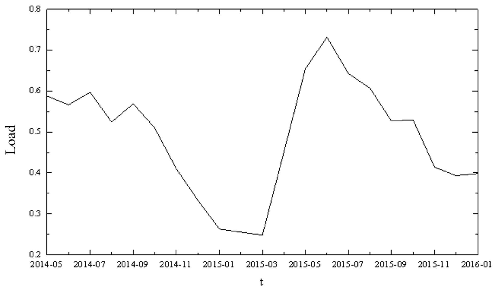
Based on the data collected by the vehicle weighing system of the cable-stayed bridge from May 2014 to January 2016 (as shown in Figure 3), the future load prediction can be realized based on the above wavelet neural network method. Taking the collected data as the sample value of the training network, according to the vehicle statistics of the cable-stayed bridge, it is found that the equivalent vehicle load in a month (n) is related to the equivalent vehicle load in the previous 12 months (n − 1, n − 2, n − 3... n − 10, n − 11, and n − 12) (Qn − 1, Qn − 2, Qn − 3... Qn − 10, Qn − 11, and Qn − 12) and the number of copies in that month (m), so these 13 parameters are taken as the input value, and the equivalent vehicle load in that month, Qn, is taken as the output value.

According to the above method, the wavelet neural network is studied, and the Morlet wavelet is selected as the input excitation function. Through trial calculation, it is found that when Formula (7) is taken as 3 ($l=\sqrt{3+1}+1=3$, where t = 1), the network learning effect is the best; the total amount of learning is set to 10,000, the error target is m = 0.001, and the learning rate is $\alpha =\beta =0.01;\gamma =\eta =0.001$.

The initial parameters of the network randomly selected according to the standard normal distribution are as follows:

$$\begin{gathered} {\mathrm{w}}_{\mathrm{jk}}=\left\{\left.\begin{array}{l}-0.824 2.288 -0.852\\ 1.874 0.375 \hspace{1em}0.072\\ -4.427 -1.939 4.941\end{array}\right\}\right. \\ {\nu }_{\mathrm{k}}=\left\{\left.1.125 -1.352 3.647\right\}\right. \\ {a}_{\mathrm{k}}=\left\{\left.1.807 -0.042 0.404\right\}\right. \\ {b}_{\mathrm{k}}=\left\{\left.0.572 -0.170 1.985\right\}\right. \end{gathered}$$

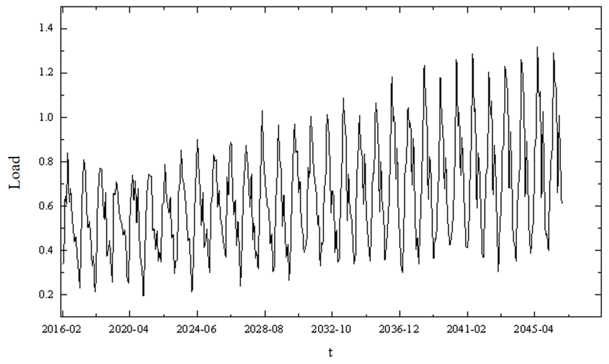
Further, the wavelet neural network method discussed in Equations (1)–(5) can be used to predict the future load model based on the existing sample library, and the vehicle load weighing system will continuously collect new data, so the sample library will also be continuously updated, and the future load prediction value is shown in Figure 4. It can be seen from the figure below that the vehicle load of the cable-stayed bridge shows a gradually increasing trend, and the seasonal difference is obvious. Because there are many mutation factors that may be generated by the vehicle load model with the change in time, only the vehicle load model between 2016 and 2046 is predicted here, and the vehicle load model after 2046 is predicted by a fixed annual increase of 5%.

4. Fatigue Damage Prognosis for Steel Main Girders of Cable-Stayed Bridges

4.1. Fatigue Reliability Model

Compared with traditional fatigue calculation methods, fatigue reliability methods can fully consider the uncertainties in external actions and structural parameters. Their essence lies in being developed based on the probability statistical distributions of external actions and structural parameters, and the obtained fatigue life predictions are probability distributions with statistical significance. In the fatigue damage prognosis process for steel structures, various types of uncertain factors are prevalent, making deterministic prognosis results meaningless. Results considering uncertainties with certain reliability levels are more convincing; thus, reliability methods are effective in fatigue damage prognosis. Current fatigue reliability analysis methods primarily include fatigue cumulative damage models, residual strength models, and fatigue life models.

Based on the fatigue cumulative damage model, the fatigue damage reliability limit state equation can be obtained:

$$g(X)=D_c-D(n)$$

(10)

Here, $D_c$ represents the critical fatigue damage threshold of the structure, and $D(n)$ denotes the cumulative fatigue damage under n cyclic load cycles. When $D(n)<D_C$, the structure remains in the fatigue-safe state (i.e., it has not reached the fatigue limit state). When $D(n)>D_C$, the structure enters the fatigue-failure state (i.e., fatigue damage has occurred). The fatigue failure probability, $p_f$, and fatigue reliability index, $\beta$, can be calculated as:

$$p_f=p[g(X)<0]$$

(11)

$$\beta ={\mathrm{\Phi }}^{-1}(1-p_f)=-{\mathrm{\Phi }}^{-1}(p_f)$$

(12)

where $\mathrm{\Phi }$ is the standard normal cumulative distribution function.

Based on the S-N curve and Miner’s linear cumulative damage criterion,

$$D={\displaystyle \sum _{i=1}^n\frac{n_i}{N_i}}={\displaystyle \sum \frac{{\alpha }_i}{C}}\cdot {\displaystyle \frac{N}{S_i^{-m}}}={\displaystyle \frac{N}{C}}{\displaystyle \sum [{\alpha }_i\cdot S_i^m]}={\displaystyle \frac{N}{C}}{S}_{eq}^m$$

(13)

where C and m are curve constants (the parameters of the S-N curve equation); $n_i$ is the actual number of cycles under stress amplitude, $S_i$ (the cumulative cycles observed in service); $N_i$ is the ultimate number of cycles calculated from the S-N curve under stress amplitude, $S_i$ (the cycles to failure under constant amplitude loading); D is the damage accumulation ratio, defined as the ratio of the actual cumulative total cycles, N, to the predicted failure cycles (critical threshold for fatigue failure); and $S_{eq}$ is equivalent stress amplitude, $S_{eq}=\sqrt[m]{{\displaystyle \sum {\alpha }_i\cdot S_i^m}}$.

In this paper, considering the monthly variation in traffic volume, $a_{ij}$ is the variation coefficient of the equivalent vehicle load in the j month after the i year, and $n_j$ is the number of daily cycles in the j month, so the fatigue limit equation can be expressed as

$$g(X)=D_c-{\displaystyle \sum _{i=1}^n{\displaystyle \sum _{j=1}^{12}30\cdot n_i\cdot a_{ij}\cdot S_{eqj}^m/C}}$$

(14)

As shown in Equation (14), the fatigue reliability of a structure is determined by its material properties and external load conditions. Specifically, the fatigue failure critical threshold, $D_c$, and fatigue detail parameters, C and m, are primarily governed by the material properties of the structure. The equivalent stress amplitude, $S_{eq}$, and equivalent stress cycle count, $n_i$, depend on both the material properties and external fatigue loads.

In the calculation of structural fatigue reliability, it is particularly critical to determine the parameters related to fatigue. In this section, based on research results at home and abroad, considering the uncertainty of materials, a fatigue reliability assessment is carried out.

$D_c$ is the critical value of the fatigue cumulative damage, which can be set to follow the lognormal distribution of the mean value $u=1$ and coefficient of variation $\sigma =0.3$.

C and m are the curve constant terms, characterizing the fatigue details of the material. Due to the small variability of M, for the convenience of engineering applications, it is often chosen as a constant representative value: m = 3. Based on the code for the design of highway steel structure bridges (JTG d64-2015) [25] and the design documents of cable-stayed bridges, it can be determined that the fatigue detail category is 80, so it can also be set to obey the logarithmic positive distribution of the mean value $u=1.024\times {10}^{12}{\left(\mathrm{Mpa}\right)}^3$ and the coefficient of variation $\sigma =0.45$.

$S_{eq}$ and $n_i$ are the equivalent fatigue stress amplitude and number of stress cycles. At present, the calculation methods widely used in the engineering field are (1) based on the stress and strain sensor; the real-time stress and strain data of the real bridge are collected, and then, the representative values are directly calculated by combining the calculation formulas. (2) They are also based on the vehicle load data collected by the WIM system; it is applied to the finite element model. Firstly, the stress time history data of the bridge are calculated, and then, its representative value is indirectly calculated by combining it with the calculation formula. The former calculation is simple and direct, but it is greatly affected by the measured signal, and due to the limited number of sensors, it is impossible to calculate the fatigue reliability of the whole bridge. Considering the limited strain data of the steel girder collected by the cable-stayed bridge health monitoring system, this paper uses the second method to study the fatigue damage prognosis of the steel girder of the cable-stayed bridge.

4.2. Fatigue Load Effect and Reliability Calculation Method

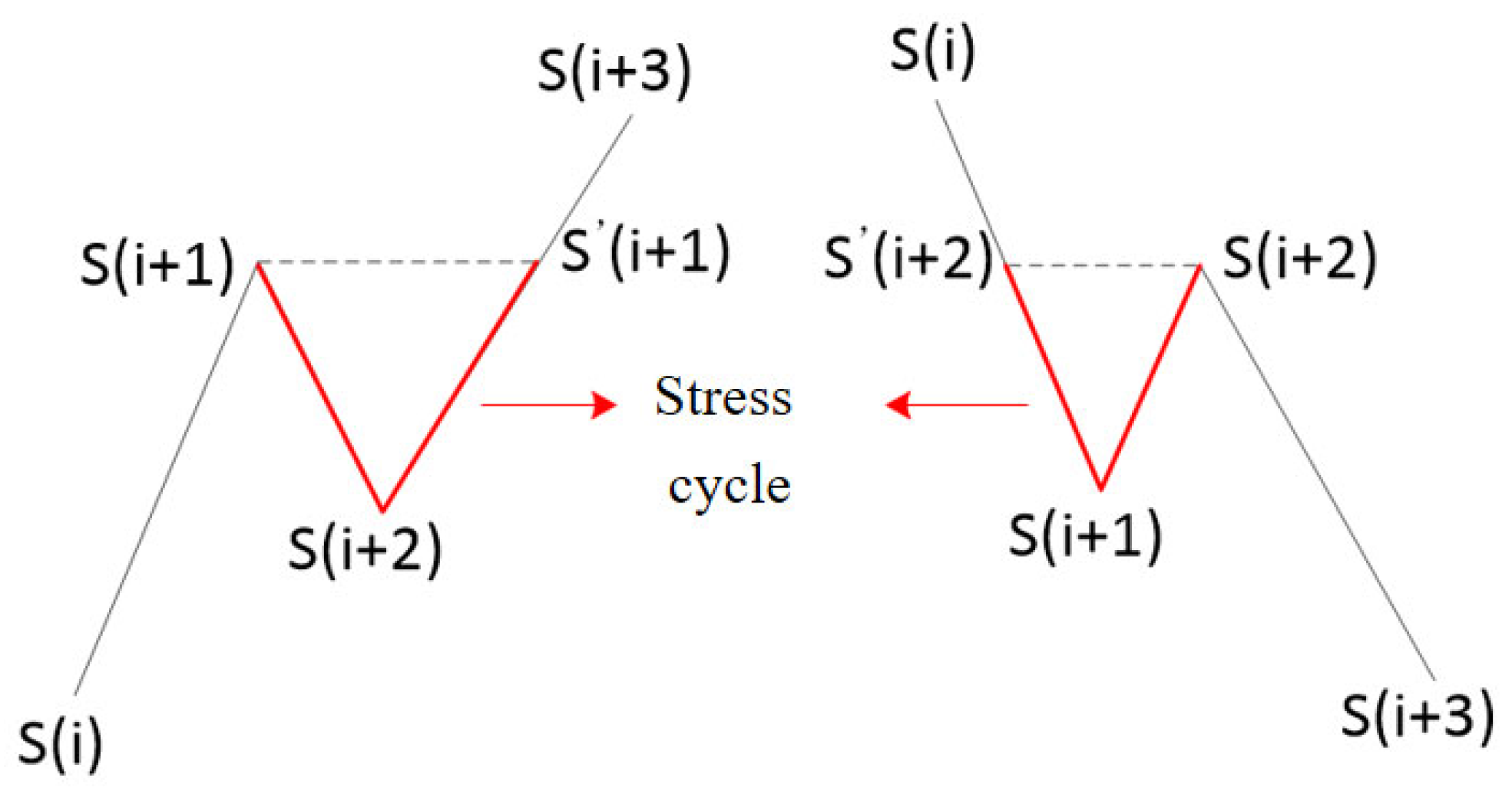
Based on the measured vehicle load model and the finite element model, the stress time history of the key nodes of the steel girder of the cable-stayed bridge is calculated. In order to calculate the equivalent fatigue stress amplitude, $S_{eq}$, and the number of stress cycles, $n_i$, the rain flow counting method is used to extract the stress amplitude and the corresponding number of stress cycles at different levels and convert them into the equivalent stress amplitude and total number of stress cycles required for fatigue calculation. At present, the “four-point counting method” is widely used in engineering, which can extract the two stress cycle modes in Figure 5.

At present, the calculation methods of reliability include the first-order second-moment method, the Monte Carlo method, and the response surface method. Among them, the Monte Carlo method is the most widely used method with a certain level of accuracy and efficiency. The basic idea is to investigate the probability of an event in a large number of tests, set the combination of random variables as $x=\left(x_1,x_2,\dots ,x_n\right)$, sample n times to generate N vectors $\left(x_1^{(i)},x_2^{(i)},\cdot \cdot \cdot ,x_n^{(i)}\right)(i=1,2,\cdot \cdot \cdot ,N)$, and introduce the judgment index i:

$$I^{(i)}=\left\{\begin{array}{l}1,g(x_1^{(i)},x_2^{(i)},\cdot \cdot \cdot ,x_n^{(i)})<0\\ 0,g(x_1^{(i)},x_2^{(i)},\cdot \cdot \cdot ,x_n^{(i)})\ge 0\end{array}\right.$$

(15)

Then, the structural failure probability can be obtained as

$$p_f=p[g(X)<0]={\displaystyle \sum _{i=1}^N{I}^{(i)}}/N$$

(16)

The Monte Carlo method has a fast convergence speed and can control accuracy through the number of simulations. Generally, the failure probability of the structure is between 10⁻³ and 10⁻⁵, and the required number of samples can be estimated by the following formula:

$$N=(1-p_f)/({\delta }_{p_f}^2{p}_f)$$

(17)

where ${\delta }_{p_f}$ is the coefficient of variation of the failure probability; if the simulation accuracy is ${\delta }_{p_f}=0.1$, the sampling number is about 10⁵–10⁷, so the sampling number selected in this paper is N = 10⁶.

4.3. Fatigue Damage Prognosis of Main Girder of Cable-Stayed Bridge

The multi-scale finite element model of the cable-stayed bridge is modeled using the ANSYS software 2024R1. The bridge piers and main girders are modeled with BEAM 188 elements, while the bearings are modeled with COMBIN 14 elements. However, the midspan of the bridge is simulated using SHELL 43 elements for the main girder and SOLID 45 elements for the deck. The cable-stayed cables are modeled with LINK 8 elements, and the auxiliary structures are simulated using MASS21 to model their equivalent mass, as shown in Figure 6.

Based on the measured data of the cable-stayed bridge health monitoring system, the dynamic strain effect of the lower flange of the steel main beam in the middle span is the most obvious under the vehicle load. The arrangement of strain sensors for the steel girder at midspan is shown in Figure 7. Therefore, this paper selects the steel girder at the S39 measuring point to carry out the fatigue damage prognosis research. The multi-scale finite element model is used to calculate the dynamic influence line of each lane under the action of 1 t of unit force, as shown in Figure 8.

The fatigue load effect levels under different load levels are naturally different. In order to obtain a more realistic probability distribution of the fatigue load effect, based on the WIM system monitoring data of the cable-stayed bridge for one year, this paper restores the natural fleet information in days and loads it in the MATLAB program (R2024a) in the influence line loading mode set in Figure 8. During the loading process, the natural fleet is calculated every 1 m, and the six lanes are carried out at the same time. The daily stress time history curve at the S39 measuring point is obtained as shown in Figure 9.

Based on the vehicle load data for the effective days of the cable-stayed bridge from May 2014 to April 2015, the daily equivalent stress amplitude, $S_{eq}$, and the number of daily stress cycles, $n_i$, are calculated in days based on Formula (14). Because their probability density presents the characteristics of multimodal distribution, the Gaussian mixture distribution (GMM) is used to fit them. The results show that the four Gaussian components can basically fit the probability distribution of the sum. The parameters of the GMM fitting results of the calculated daily equivalent stress amplitude and daily stress cycle times are shown in

Table 1. Parameters of GMM fitting results for daily equivalent force amplitude and cycle times.

Time	N				Stress (MPa)
	1	2	3	4	1	2	3	4
2014.05	389.77	658.95	1235.62	1493.61	6.16	8.48	9.39	10.13
2014.06	758.65	982.02	1315.02	1613.23	6.28	8.42	8.65	9.40
2014.07	875.29	1083.54	1173.22	1682.44	7.26	8.53	9.19	10.00
2014.08	573.59	879.98	1089.01	1318.15	7.19	7.66	8.32	8.75
2014.09	354.43	865.65	1238.68	1450.81	7.04	8.15	8.72	9.52
2014.10	287.91	777.62	1090.45	1335.63	5.71	6.99	8.01	8.55
2014.11	656.74	794.93	965.84	1222.12	5.26	7.54	8.20	10.29
2014.12	607.57	677.13	935.86	1153.63	4.68	7.28	8.27	9.37
2015.01	219.03	533.14	803.53	970.96	5.23	6.12	6.33	6.42
2015.02	386.28	523.71	765.81	903.30	5.32	6.02	6.24	6.47
2015.03	164.50	534.18	769.54	886.74	4.28	5.88	6.19	6.69
2015.04	314.57	672.86	990.47	1125.31	5.14	7.13	7.65	8.58
Time	Standard deviation of N				Standard deviation of stress
	1	2	3	4	1	2	3	4
2014.05	319.21	142.62	170.27	255.27	0.00	0.75	0.21	0.76
2014.06	166.85	156.54	71.43	209.81	0.41	0.87	0.45	0.82
2014.07	277.16	175.34	163.12	73.55	0.13	0.46	0.28	0.45
2014.08	201.82	161.41	169.18	132.77	0.00	0.31	0.24	0.74
2014.09	96.44	90.79	83.42	114.56	0.10	0.40	0.44	0.78
2014.1	85.53	36.16	108.13	106.09	0.24	0.69	0.13	1.48
2014.11	149.23	174.68	86.69	104.64	0.68	0.61	0.02	0.58
2014.12	283.66	151.45	136.82	138.51	0.09	0.61	0.12	0.50
2015.01	155.05	111.81	87.15	112.07	0.11	0.54	0.38	2.95
2015.02	236.24	158.42	110.42	26.10	0.12	0.54	0.38	2.02
2015.03	32.00	105.51	187.97	31.18	0.21	0.47	0.29	0.86
2015.04	117.98	136.12	100.97	110.35	0.42	0.62	0.14	0.65
Time	Weight of n				Weight of stress
	1	2	3	4	1	2	3	4
2014.05	0.09	0.14	0.60	0.18	0.07	0.13	0.16	0.64
2014.06	0.14	0.33	0.49	0.05	0.04	0.17	0.19	0.60
2014.07	0.16	0.44	0.31	0.08	0.03	0.30	0.16	0.51
2014.08	0.16	0.29	0.28	0.27	0.07	0.18	0.20	0.55
2014.09	0.17	0.23	0.18	0.42	0.06	0.20	0.07	0.67
2014.1	0.10	0.10	0.60	0.20	0.13	0.22	0.25	0.40
2014.11	0.25	0.15	0.20	0.40	0.07	0.74	0.02	0.17
2014.12	0.17	0.25	0.32	0.25	0.07	0.69	0.10	0.13
2015.01	0.22	0.25	0.25	0.28	0.17	0.40	0.32	0.11
2015.02	0.22	0.10	0.47	0.21	0.05	0.39	0.32	0.23
2015.03	0.07	0.24	0.52	0.16	0.07	0.52	0.23	0.19
2015.04	0.16	0.31	0.17	0.37	0.07	0.50	0.22	0.21

. Using the fitting results of the probability density function and cumulative distribution function, the GMM model can effectively express the probability distribution of the fatigue load effect calculated using the actual traffic flow.

The basic assumption of the reliability calculation is that its variables obey a normal distribution. For the cumulative damage critical value, $D_c$, and constant, C, in the fatigue limit equation, their distribution is a lognormal distribution, which needs to be “equivalently normalized”. The so-called equivalent normalization means that at $X_i$, the distribution function value and probability density function value of the equivalent normal variable and the original variable are equal. For parameter $X_i$ of the lognormal distribution, it can be transformed into $X_i=e^{\ln X_i}$.

$${\mu }_{\ln X_i}=\ln {\displaystyle \frac{{\mu }_{X_i}}{\sqrt{1+{\delta }_{X_i}^2}}}$$

(18)

$${\sigma }_{\ln X_i}=\sqrt{\ln (1+{\delta }_{X_i}^2)}$$

(19)

After normalizing the nonnormal distribution variables, $D_c$ and C, the mean and standard deviation of ln$D_c$ are −0.043 and 0.294, respectively; the mean and standard deviation of lnC are 27.563 and 0.429, respectively. Furthermore, the mean value and standard deviation of $S_{eq}$ and $n_i$ after taking the weighted comprehensive value of the GMM fitting results are shown in

Table 2. Mean and standard deviation of normal variables for reliability calculation.

Time	N		Stress
	Mean	Standard Deviation	Mean	Standard Deviation
2014.05	1130.18	194.24	9.54	0.62
2014.06	1144.78	119.13	8.96	0.74
2014.07	1126.33	179.76	9.34	0.41
2014.08	1007.45	162.22	8.37	0.51
2014.09	1093.73	100.32	9.04	0.64
2014.10	1028.43	98.36	7.71	0.81
2014.11	965.30	122.91	7.85	0.60
2014.12	869.64	166.07	7.49	0.51
2015.01	653.17	115.30	6.07	0.68
2015.02	688.02	124.94	6.16	0.81
2015.03	690.87	131.64	5.99	0.49
2015.04	836.38	117.95	7.42	0.51

. The mean value of the equivalent stress amplitude is in the range [5.99–9.54 MPa], and the mean number of stress cycles is in the range [653.17–1144.78]; the seasonal difference is obvious. The daily equivalent stress amplitude and the number of daily stress cycles from May to July are larger, and the stress is smaller from January to March, which matches the seasonal difference in traffic flow.

Target reliability, ${\beta }_T$, is the minimum safety level of a structure recognized in a particular field. Because it is intuitive and convenient, it is generally used as a standard to judge whether a structure is invalid. Based on various research results, the target fatigue reliability index in this paper is 3.5, and the corresponding failure probability is 0.13%.

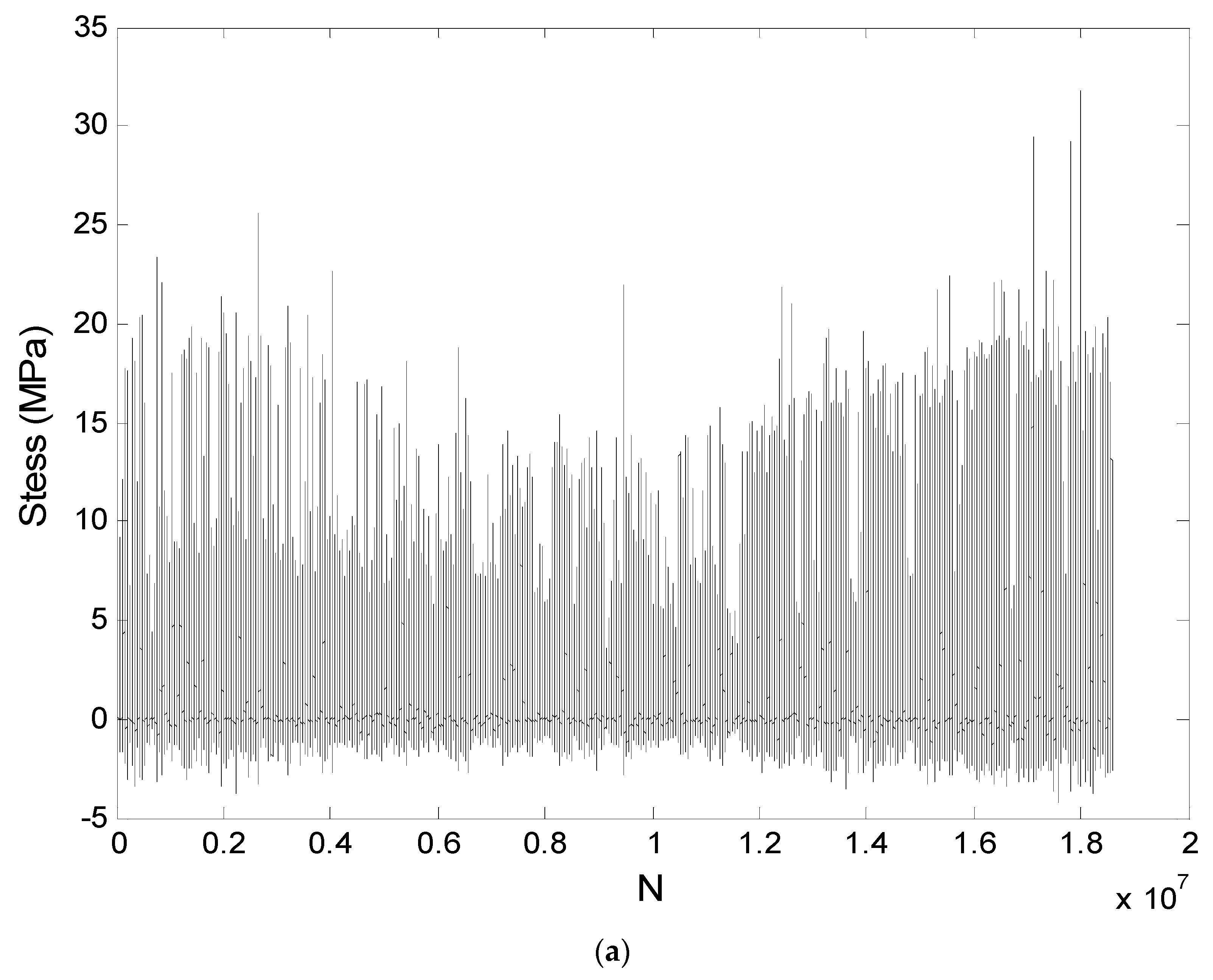
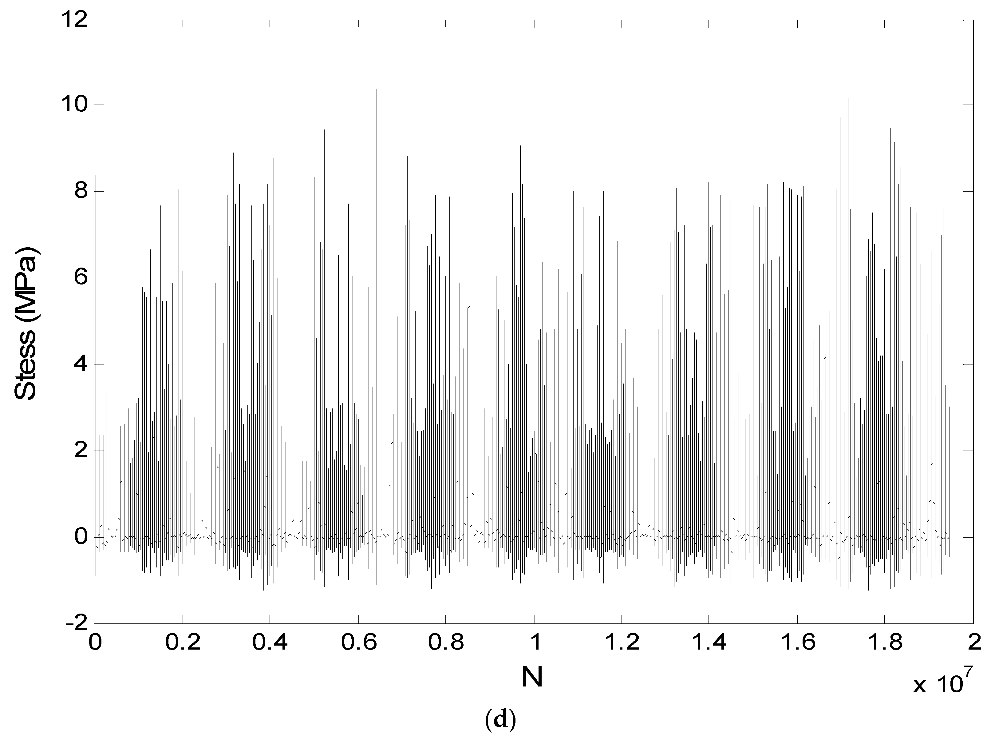
The fatigue reliability and failure probability of key fatigue parts of a cable-stayed bridge calculated by the Monte Carlo method are shown in Figure 10, based on the fatigue load effect from May 2014 to April 2015 and combined with the prediction results of a wavelet neural network for a future vehicle load model. The calculation results show that

(1)

The fatigue reliability of the bridge within a design service life of 100 years decreases rapidly, but it is at a high level. The calculated fatigue reliability at the end of service is 5.19, which is higher than the target fatigue reliability of 3.5, and the failure probability is 1.03 × 10⁻⁷. The failure probability is very small. At this time, the fatigue performance of the bridge is still in a reliable state.

(2)

The service life of the cable-stayed bridge is about 152 years when it reaches the target fatigue reliability. After that, the fatigue reliability decreases slowly, but the failure probability increases greatly, and the structural fatigue performance is in an unreliable state.

5. Conclusions

Based on the data-driven method, combined with the multi-scale finite element model, the fatigue damage prognosis of the main girder of a cable-stayed bridge was studied in this paper.

(1)

Based on the wavelet neural network method, the future load model prediction based on the existing sample database can be completed. The prediction results show that the vehicle load of the cable-stayed bridge shows a gradual growth trend, and the seasonal difference is obvious.

(2)

Based on the measured vehicle load, the fatigue equivalent stress amplitude and the number of stress cycles per day of the cable-stayed bridge can be obtained. The average value of the equivalent stress amplitude is in the range [5.99–9.54 mpa], and the average number of stress cycles is in the range [653.17–1144.78]; the seasonal difference is obvious. The daily equivalent stress amplitude and the number of daily stress cycles from May to July are larger, and the stress is smaller from January to March, which matches the seasonal difference in traffic flow.

(3)

The results of the fatigue damage prognosis of the cable-stayed bridge show that the fatigue reliability of the bridge within a design service life of 100 years decreases rapidly, but it is at a high level. The calculated fatigue reliability at the end of service is 5.19, which is higher than the target fatigue reliability of 3.5, and the failure probability is 1.03 × 10⁻⁷. The failure probability is very small. At this time, the fatigue performance of the bridge is still in a reliable state. The service life of the cable-stayed bridge is about 152 years when it reaches the target fatigue reliability. After that, the fatigue reliability decreases slowly, but the failure probability increases greatly, and the structural fatigue performance is in an unreliable state.