Abstract
Prefabricated components inevitably generate numerous assembly joints during installation, with each 1 mm increase in joint width correlating to a 15–20% elevation in the annual occurrence frequency of the frost formation risk. In the Inner Mongolia Region, the water migration at wall connection interfaces during winter significantly exacerbates freeze–thaw damage due to persistent thermal gradients. A coupled heat–moisture transfer model incorporating gas–liquid–solid phase transitions was developed, with the liquid moisture content and temperature gradient as dual driving forces. A validation against internationally recognized BS EN 15026:2007 benchmark cases confirmed the model robustness. The prefabricated sandwich insulation walls reconstructed with region-specific volcanic ash materials underwent a comparative evaluation of temperature and relative humidity distributions under varied winter conditions. Furthermore, we analyze and assess the potential for freezing at connection points and identify the specific areas at risk. Synergistic effects between assembly gaps and indoor–outdoor environmental interactions on wall performance degradation were systematically assessed. The results indicated that, across all working conditions, both the temperature and relative humidity at each wall measurement point underwent periodic variations influenced by the outdoor environment. These fluctuations decreased in amplitude from the exterior to the interior, accompanied by a noticeable delay effect. Specifically, at Section 2, the wall temperatures at points B2–B8 were higher compared to those at A2–A8 of Section 1. The relative humidity gradient remained relatively stable at each measurement point, while the temperature fluctuation amplitude was smaller by 2.58 ± 0.3 °C compared to Section 1. Under subfreezing conditions, Section 1 demonstrates a marked reduction in relative humidity (Cases 1-3 and 2-3) compared to reference cases, which is indicative of internal ice crystallization. Conversely, Section 2 maintains higher relative humidity values under identical therma. These findings suggest that prefabricated building joints significantly impact indoor and outdoor wall temperatures, potentially increasing the indoor heat loss and accelerating temperature transfer during winter.
1. Introduction
In recent years, alongside the advancing development of building energy conservation and the embrace of sustainable development concepts, the issue of freezing and thawing affecting prefabricated building envelopes in winter, particularly in the northern cold regions of China, has emerged as an urgent aspect to address. Variations in the indoor and outdoor temperature, humidity, and air pressure significantly impact the thermal performance of the building envelope [1]. Furthermore, with changes in the climate environment, the heat and moisture transfer tendencies within walls can increase by over 10% [2]. Compared with monolithic cast-in-place walls, the discontinuous interfaces formed by assembly joints in precast concrete structures not only degrade the thermal insulation performance and durability, but also disrupt the internal pore structure of concrete materials, consequently altering hygrothermal transport pathways and phase-change characteristics. Therefore, the precise analysis of hygrothermal transport at precast building joints can enhance the thermal performance of prefabricated wall systems by 12–18% through optimized joint design [3]. This study pioneers the development of a coupled heat and moisture transfer model for prefabricated wall joints under transient freeze–thaw cycling boundary conditions, specifically adapted to the severe cold and alternating dry–wet climate patterns of Inner Mongolia. By developing a thermal–moisture–air multifield coupling simulation platform, we have addressed the critical challenge of the dynamic moisture transfer simulation in prefabricated wall joints specific to Inner Mongolia’s climatic conditions. Furthermore, an innovative wall joint system utilizing locally sourced volcanic slag aggregates has been proposed, achieving dual benefits in environmental sustainability and high-efficiency applications.
In the field of heat and mass transfer in prefabricated building materials, Chen Y J et al. [4] found that when filled with aerated blocks, the joints were most significantly affected by moisture migration, with a heat flux loss rate of 8.08%. Under high-temperature conditions, the thermal performance at composite wall connections was particularly susceptible to humidity effects, showing heat flux loss rates ranging from 6.17% to 8.74%. Yang Y T [5] investigated hygrothermal migration phenomena in novel prefabricated sandwich exterior wall panels secured with basalt fiber-reinforced polymer (BFRP) connectors. Ji J J [6] found that bolt connections exerted a more pronounced impact on the wall thermal performance and moisture migration than grouted sleeve connections. Zhao, GQ et al. [7] introduced a novel prefabricated cold-formed light steel stud wallboard, using a structural silicone sealant to join steel studs with steel plates. MC’s [8] study demonstrated that, despite the reduced steel usage in a standard modern sandwich panel, the thermal resistance of the wall panel can be decreased by 38% when the steel connector bridge plate only occupies 0.08% of the area. Kraus M [9] conducted experimental measurements of the indoor air temperature and relative humidity in prefabricated panel houses located in Ostrava, Czech Republic, during both non-heating and heating seasons. Xue Y C et al. [10] revealed that the insulation layer may elevate the moisture content within the wall–floor thermal bridge (WFTB) zone, and increasing the insulation could increase the overall thermal conductivity of the WFTB.
Many scholars, both domestically and internationally, have focused on the coupled heat and moisture transfer process within building envelopes. Significant efforts have been made in theoretical research, computational methodologies, and simulation tools. In the early 20th century, scholars conducted extensive research on moisture transfer in porous media, progressively establishing and refining coupled heat and moisture transfer models for wall assemblies using temperature and relative humidity as driving potentials. Philip and de Vries [11] posited that moisture transfer occurs in both gas and liquid phases. Their examination of soil moisture transfer led them to introduce the inaugural heat and moisture transfer model, which integrates heat and moisture, with moisture and temperature serving as the driving potential. H. M. Künzel [12] and other researchers have taken into account the capillary effect, diffusion, moisture absorption, and desorption of water within walls. They have established a coupled model for heat and moisture transfer, with relative humidity serving as the driving potential. However, because of the intricate existence and transfer processes of wet components, various scholars possess differing driving potentials and assumptions when establishing models, thus leading to certain limitations in their research models. In recent years, Feng Chi [13] has elucidated the mathematical and physical relationships involved in their mutual conversion. This was achieved by deriving transfer and conservation equations rooted in diverse driving potentials and subsequently comparing their respective advantages and disadvantages. Wang Y Y et al. [14] analyzed the transient coupled heat and moisture transfer process within wall assemblies using relative humidity and temperature as driving factors and calculated the temperature, humidity, and heat flux density at wall surfaces. Meanwhile, DONG W Q et al. [15] validated the coupled heat and moisture transfer processes within porous building materials and envelope structures. They achieved this by comparing FORTRAN code outputs and COMSOL Multiphysics 6.1 simulation results against analytical solutions and various other datasets. Qin, M et al. [16] employed the vapor content and temperature as driving potentials to develop a mathematical model addressing coupled heat and moisture transfer phenomena in multilayered porous building materials.
Finding a universal model for the coupled heat and moisture transfer across various regions and porous materials remains challenging. As a result, numerous specialized heat and moisture transfer (HAMT) models are consistently emerging. Notably, LIU et al. [17] developed and validated a multi-coupled transient analysis model involving heat, moisture, and air transfer, revealing temperature distribution patterns, humidity variations, and heat flux density characteristics at the interface between expanded polystyrene (EPS) insulation systems and concrete substrates. Bagaric M et al. [18] conducted hygrothermal performance experiments on ventilated recycled concrete sandwich composite panels, confirming that air movement across south-oriented panel surfaces significantly enhances their thermo-hygric regulation capacity. Li et al. [19] employed the WUFI® Pro software to conduct hygrothermal performance simulations on bamboo exterior wall systems across five major climate zones. The simulation results revealed that the bamboo scrimber (BS) material demonstrated a superior heat storage capacity compared to laminated bamboo lumber (BLL), whereas the BLL exhibited a relatively higher moisture buffering capability. Meanwhile, Cai Shanshan [20] and associates proposed a multi-scale model to explore the influence of the internal structure on dynamic heat and moisture transfer processes. Furthermore, they employed a neural network algorithm to anticipate the effects of the internal structure of closed-cell insulation (phenolic) on these dynamic transfers, grounded on the effective transmission coefficient at the mesoscopic scale.
In cold and severe cold regions, Matsumoto [21] and colleagues developed a mathematical model for coupled heat and moisture transfer in concrete undergoing freezing and thawing processes, utilizing the wet chemical potential as the driving force. Kong F H et al. [22] accounted for the permeability and freezing characteristics of liquid water in porous building materials and formulated conservation equations for coupled heat and moisture transfer under varying transport conditions, and this model can simulate the hygrothermal coupling in newly constructed building envelopes in severe cold regions. Wang Y et al. [23] developed a transient coupled hygrothermal model based on existing theories of heat and moisture transfer in walls to simulate the hygrothermal transport process and calculated heat transfer during winter insulation periods. Shen X W et al. [24] demonstrated that the majority of liquid water accumulated within the concrete layer, while freeze–thaw cycles and temperature gradient development predominantly occurred within the insulation layer; the combined effect of the moisture content and ice formation resulted in average increases of 15.5% and 14.6%, respectively, in thermal transmittance for both EPS panel cast-in-place concrete and EPS panel lightweight concrete external thermal insulation composite systems (ETICSs) compared to dry conditions.
Currently, research on the performance of prefabricated buildings, both domestically and internationally, primarily centers around the thermal performance of walls, connectors, and thermal bridges from the standpoints of mechanical structures and thermal insulation. However, there is a notable gap in the exploration of how heat and moisture transfer at the joints is affected by the unique construction methods inherent to prefabricated buildings. Furthermore, studies on the heat and moisture coupling characteristics of connection joints remain insufficient. Additionally, within the broader context of research on heat and moisture transfer in building envelopes, the majority of studies only account for the internal water vapor–liquid phase transition, while research on internal wall freezing in severe cold regions remains limited. This paper aims to develop a coupled heat and moisture transfer model for prefabricated buildings in severe cold regions. Through a numerical simulation, this study will examine the heat and mass transfer process of a new prefabricated concrete sandwich insulation wall during winter in Hohhot. The objective is to obtain the temperature and humidity field, as well as the heat flux density within the structure, and to further analyze how moisture transfer characteristics impact the thermal and moisture performance of the prefabricated wall.
2. Mathematical Model
2.1. Physical Model
Based on the law of the conservation of energy and mass, a one-dimensional physical model of the wall, as depicted in Figure 1, has been established, satisfying the following assumptions:
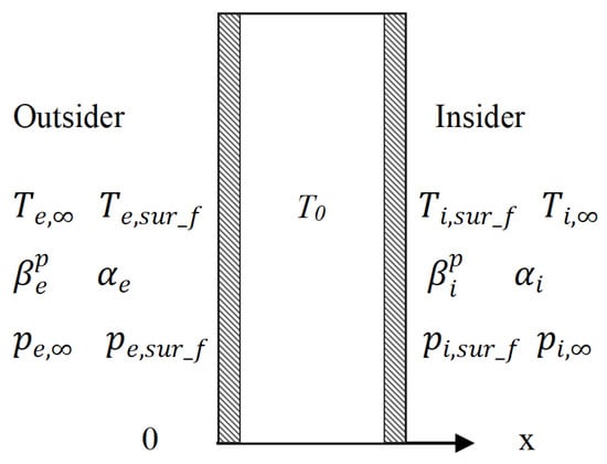
Figure 1.
Wall physical model and boundary conditions.
- (1)
- The building material constitutes an isotropic, continuous, and homogeneous porous medium that exhibits no deformation of its solid skeleton and remains undeformed even when frozen.
- (2)
- The moisture present in the porous media material comprises three phases, gas, liquid, and solid, where each phase maintains local heat and moisture equilibrium in the absence of chemical reactions.
- (3)
- The gas phase, comprising air and water vapor, is regarded as an ideal gas. The flow dynamics of both the gas and liquid phases adhere to Darcy’s law, while ice remains stationary.
- (4)
- Neglecting the impact of air infiltration within the wall, it is assumed that heat and moisture solely migrate along the wall’s thickness.
- (5)
- Given the intimate contact between the materials of each layer, the moisture transfer resistance and contact thermal resistance are disregarded.
Based on the aforementioned fundamental assumptions, in accordance with the law of the conservation of energy and mass, the temperature gradient has been chosen as the driving potential for heat transfer, while the volume water content gradient has been selected as the driving potential for moisture transfer. Subsequently, a mathematical model for the heat and mass transfer within the wall has been established.
2.2. Initial Conditions
Assuming that at t = 0, the temperature field, volume moisture content field, and solid ice content field are as follows:
2.3. Mass Conservation Equation
The prefabricated wall can be conceptualized as a cube. Consider any microelement V, and the mass of a phase within the characterization element Rev is given by
Based on the principle of mass conservation, the mass increment ∆ma of a specific phase α within the characterization voxel during the time interval ∆t is equivalent to the combined mass of the α phase flowing through the Rev boundary within ∆t and the mass of the α phase generated within the rev.
Through differentiation with respect to time t in Equations (2) and (3), we can derive the following:
Using the Divergence Theorem [25], we have , Equation (4) can be simplified to
Assuming that the ice body remains stationary, the mass conservation equation encompassing the water vapor, liquid water, and solid ice is as follows:
When the moisture transport attains equilibrium, the combined rate of the liquid water generation, water vapor, and solid ice phase equals 0, with , , .
Generally, the gas-phase convection inside the wall can be disregarded, and the mass conservation equation stands as follows:
When there is no freezing phenomenon inside the wall, specifically when the ice phase content is , , the formula is as follows:
When icing occurs within the wall pores, the mass conservation equation can be formulated as follows:
Once the liquid water within the wall’s pores is fully frozen, the mass conservation equation can be formulated as follows:
2.4. Energy Conservation Equation
Based on the law of the conservation of energy, if we consider that the total energy variation within the control body is equivalent to the combined heat flow resulting from the heat conduction, moisture transfer, and migration, as well as the internal heat source, then the following can be derived:
The latent heat associated with the phase change during the wet migration process is considered as the heat released by the internal heat source. To illustrate, let us take the steam liquefaction process as an example.
When the porous medium experiences only a gas–liquid phase transition, solid ice remains adhered to the skeleton. By substituting Equations (12) and (13) into Equation (11), we obtain an energy equation that solely accounts for the gas–liquid phase transition.
When the liquid–solid phase transition takes place within building materials, this paper disregards the vapor–solid phase transition process in comparison to the solid–liquid phase variables. The phase transition process is shown in Figure 2. For instance, consider the icing process
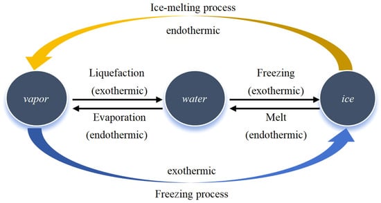
Figure 2.
Schematic diagram of three-phase transition of gas, liquid, and solid.
Based on the gas–liquid two-phase transition, we incorporate the internal heat source term associated with liquid water freezing. By integrating Equations (12), (13) and (16) into Equation (11), we derive the energy conservation equation for the gas, solid, and liquid three-phase transition:
2.5. Boundary Conditions
- (1)
- Indoor boundary conditions:
Mass boundary condition:
Energy boundary conditions:
represents the indoor water vapor exchange coefficient (s/m), and represent the partial pressure of the water vapor on the indoor wall surface and in the surrounding environment, respectively, pa. represents the indoor heat exchange coefficient (W/m2·k), and and represent the indoor wall surface temperature and ambient temperature, respectively, in °C.
- (2)
- Outdoor boundary conditions
Mass boundary condition:
Energy boundary conditions:
represents the outdoor water vapor exchange coefficient (s/m), and represent the partial pressure of the water vapor on the outdoor wall surface and in the surrounding environment, respectively, pa. represents the outdoor heat exchange coefficient (W/m2·k), and and represent the outdoor wall surface temperature and ambient temperature, respectively, in °C.
Based on relevant thermal and moisture theories, this paper formulates assumptions for a model that considers both the moisture content gradient and temperature gradient as driving forces. It comprehensively accounts for the gas, solid, and liquid phase transitions of water within porous building materials specific to Inner Mongolia. Consequently, a dynamic model for the coupled heat and moisture transfer in porous media walls of this region is established. The model incorporates various influencing factors, including heat transfer, moisture transfer, and their interactions, providing an accurate representation of the complex heat and moisture coupling transfer mechanism. Furthermore, it addresses the three-phase moisture transition process (gas, solid, and liquid) within the connecting joints of prefabricated buildings in the area. Utilizing the driving forces of the moisture content and temperature gradients, a mathematical framework for heat and moisture coupling transfer is devised. This framework integrates crucial components that impact the moisture–heat interaction, such as heat conduction, water diffusion, and their dynamic coupling effects. It resolves numerical challenges arising from the discontinuous liquid migration at interfaces. Additionally, the model takes into account the influence of ice crystallization’s phase change enthalpy on the liquid water transport within the pores of wall materials. As a result, mass and energy conservation equations are derived for three distinct states within the wall material pores: no freezing of liquid water, partial freezing, and complete freezing.
3. Numerical Simulation
Coupled heat and moisture transfer simulations were performed on two sets of prefabricated joint connections using COMSOL Multiphysics 6.1. The main wall dimensions were 0.8 m × 0.6 m, with a predefined triangular mesh element scheme (extremely fine) applied for meshing. A local refinement with three-layer boundary layers was implemented in the joint regions (minimum element size 0.005 m). The grid independence was verified through a coarse–medium–fine mesh triplet comparison. The mesh independence was confirmed when the coefficient of variation (CV) of the moisture flux density at joints fell below 2%. An implicit coupled solver with Newton–Raphson iterations (maximum iterations 50, damping factor 0.7) was employed to resolve nonlinear coupling effects. Temporal discretization utilized the second-order backward differentiation formula (BDF2) with an initial time step of 3600 s and a maximum step of 86,400 s. Adaptive time-stepping controlled the temporal resolution during ice phase-change stages (Δt/τ < 1%). Convergence criteria required a simultaneous reduction in dual-field residuals to a relative tolerance of 1 × 10⁻⁴, with absolute tolerances set to 0.1 K (temperature) and 0.01 kg/m3 (humidity).
3.1. Simulation Verification
The proposed heat moisture coupling transmission model is constructed using the COMSOL multiphysics partial differential equation (PDE) module, and the simulation research is conducted in alignment with the BS EN15206 international standard to evaluate the mathematical model’s accuracy. The BS EN 15026 [26] validation case examines the heat and moisture transfer processes within a semi-infinite structural concrete wall, whose geometric structure is depicted in Figure 3, while the material heat and moisture parameters of the structure are detailed in Table 1.
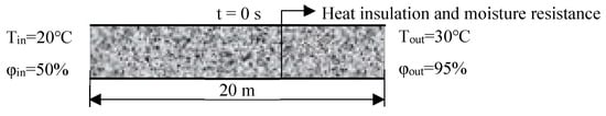
Figure 3.
Geometry of concrete walls.

Table 1.
Parameters of semi-infinite concrete structures.
The wall’s initial temperature stands at 20 °C (293.15 k) with a relative humidity of 50%. At t = 0 s, the inner boundary experiences an ambient temperature increase to 30 °C (303.15 k) and a relative humidity of 95%. Meanwhile, the outer boundary maintains its initial temperature and humidity levels, while the upper and lower interfaces are moisture-insulated. By importing the standard data from BS EN 15206, simulations of heat and moisture distribution were conducted for 7, 30, and 365 days. A comparison between these simulation results and case test data is presented in Figure 4.
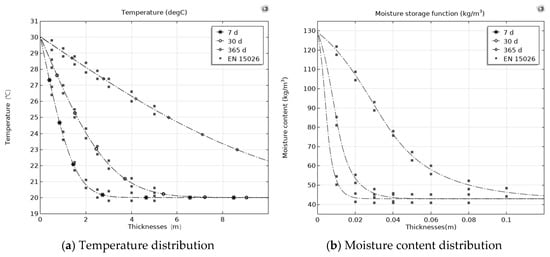
Figure 4.
Comparison between simulation results and standard verification.
As evidenced by the simulation results, the distributions of both the temperature and moisture storage capacity exhibit a close agreement with the computational outcomes derived from the BS EN 15206 standard, with a maximum relative error of 1.79%, thereby validating the accuracy of the proposed model.
3.2. Simulation Calculation
3.2.1. Wall Structure
Given the complex heat and moisture transfer dynamics along the joint interface of this wall, we conducted calculations and analyses across various sections. We compared the heat and moisture transfer at the interfaces of different materials and examined the impact of the prefabricated assembly joint on the wall’s temperature and humidity. The simulated wall has an overall thickness of 270 mm, comprising a 50 mm outer leaf wall, a 70 mm insulation layer, and a 150 mm inner leaf wall. For Section 1, we placed 10 points on the wall at distances of 0, 25, 50, 85, 120, 175, 225, 270, 400, and 600 mm from the inner wall surface. For Section 2, there are eight points located at distances of 0, 25, 50, 85, 120, 175, 225, and 270 mm from the inner wall surface. Please refer to Figure 5 for a detailed illustration of the wall structure and the distribution of points.
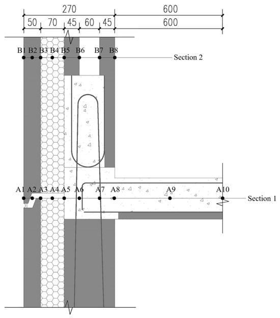
Figure 5.
Wall structure and measurement point distribution dimensions of different layers.
The construction materials for Sections 1 and 2 are illustrated in Figure 6a and Figure 6b, respectively. In contrast to Section 2, Section 1 features a high–low joint inverted sill structure. The comparison was made regarding the heat and moisture transfer of diverse structural walls at the junction of various materials.
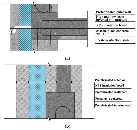
Figure 6.
(a) Section 1 construction material. (b) Section 2 construction material.
The interface of Section 1 transitions from the outside to the inside as follows: the exterior wall surface, high–low joint inverted sill structure, prefabricated outer leaf wallboard insulation layer, high–low joint insulation layer, insulation layer at the cast-in situ concrete interface, cast-in situ concrete, reinforcement, and, finally, cast-in situ floor slab. Please refer to Table 2 for the structural materials corresponding to the specific measurement points.
Table 2.
Measurement point parameters for Section 1 wall.
Section 2 pertains to the exterior wall surface, specifically addressing the prefabricated exterior leaf wallboard, its insulation layer (XPS), the relation of the insulation layer to the prefabricated wallboard, the connection between the prefabricated wallboard and the cast-in situ concrete, the linkage of the cast-in situ concrete to the prefabricated inner leaf wallboard, and finally, the interior wall surface. For detailed construction materials at specific measurement points, please refer to Table 3.
Table 3.
Wall measuring point parameters of Section 2.
3.2.2. Concrete Raw Materials
Inner Mongolia is home to a vast quantity of natural volcanic slag. The specific volcanic slag employed in this simulation originates from the Huitenghe region of Ximeng, alongside CL20. Refer to Table 4 for the optimal mix proportions of volcanic slag concrete pertaining to CL25 and CL30.
Table 4.
Mix proportion for volcanic slag concrete [27].
Pozzolanic concrete consists of cement, pozzolanic material, sand, and water. Compared to traditional concrete, pozzolanic concrete stands out due to its light weight, porous structure, low thermal conductivity, and thermal insulation properties. Its density is significantly lower than that of regular concrete, specifically about 20 to 35% less than C30 ordinary concrete. Furthermore, its thermal conductivity is decreased by over 50%, while its durability—including its impermeability and frost resistance—is enhanced by 30 to 50%. Leveraging these advantages, the pozzolanic material available in this region is employed as the foundational material for walls and is combined with thermal insulation material. This creates a novel fabricated sandwich insulation exterior wall panel structural joint for simulation research purposes. Refer to Table 5 for detailed physical parameters of the simulated wall materials.
Table 5.
Physical parameters of wall materials.
3.2.3. Calculation Conditions
In the majority of previous studies, researchers frequently utilized constant indoor and outdoor temperature and humidity values, which fell short in precisely simulating the continual variations in the actual environmental wall temperature and relative humidity. To delve into the migration process of the temperature and humidity within the outer retaining walls of buildings located in severe cold regions, this paper aims to examine the distribution of temperature and humidity within the wall, along with its influencing factors, by taking measurements of the outdoor hourly temperature and relative humidity shifts during the winter month of January in Hohhot, Inner Mongolia, under real climatic conditions.
The average outdoor air temperature in January 2023 during winter stands at −12.81 °C, with an average relative humidity of 68.2%, as illustrated in Figure 7. As per the code for the thermal design of civil buildings, the indoor temperature of heated rooms in winter is set at 18 °C, with a relative humidity of 60%. The initial indoor and outdoor temperatures are 15 °C and 0 °C, respectively, the initial wall temperature is 0 °C, while the initial indoor and outdoor relative humidity levels are 30% and 60%, respectively.
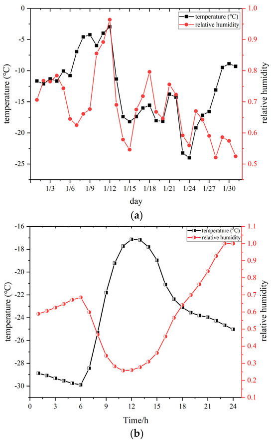
Figure 7.
(a) Outdoor temperature and humidity change curve in January 2023 during winter. (b) Temperature and relative humidity changes on 1 January 2023.
3.2.4. Simulated Working Conditions
Based on the actual indoor and outdoor thermal and humidity conditions in severe cold regions, as well as the data parameters of wall materials in this area, this study examines how changes in the indoor and outdoor temperature and relative humidity affect the heat and moisture transfer and thermal performance of prefabricated walls. To this end, six distinct winter temperature and humidity scenarios are simulated (refer to Table 6). Each scenario ensures a relative stability in the wall’s temperature and relative humidity, maintaining these conditions for over 72 h before proceeding to the next operational state.
Table 6.
Temperature and humidity parameters under different working conditions during winter.
To investigate the impact of changes in the internal temperature of the wall on the heat and moisture transfer, the winter operating conditions for simulation group 1 were established as follows: the indoor temperature and relative humidity remained constant while the outdoor temperature was gradually reduced from 0 °C to −20 °C in increments of 10 °C, with no changes in relative humidity. These conditions correspond to operating scenarios 1-1 through 1-3, respectively.
To investigate the effects of indoor and outdoor temperature and relative humidity variations on the heat and moisture transfer of the wall, the winter outdoor measured average temperature (conditions 1-2) was used as a benchmark. Different environmental parameters were compared and calculated for simulation group 2. Specifically, condition 2-1 involved no changes in indoor and outdoor temperatures while varying the relative humidity (from 60% to 40% outdoors and from 30% to 20% indoors). Condition 2-2 entailed a shift in indoor and outdoor temperatures (outdoor temperature decreased from −10 °C to −15 °C, and indoor temperature dropped from 15 °C to 10 °C) while maintaining constant relative humidity. Lastly, condition 2-3 encompassed changes in both the indoor and outdoor temperature and relative humidity (outdoor temperature and humidity were set to −30 °C and 70%, and indoor temperature and humidity were adjusted to 5 °C and 40%).
4. Results and Discussion
4.1. Temperature Variations at Wall Measurement Points
4.1.1. Temperature Fluctuations in Section 1 Across Diverse Operating Conditions
Figure 8 illustrates the temperature distribution over time of the points within the wall of Section 1 across six working conditions. Specifically, Figure 8a corresponds to working conditions 1-1, Figure 8b to 1-2, Figure 8c to 1-3, Figure 8d to 2-1, Figure 8e to 2-2, and Figure 8f to 2-3. Under varying working conditions and influenced by the outdoor temperature, each point within Section 1’s wall exhibits irregular periodic temperature changes. These temperature waveforms roughly mirror those of the external environment. Notably, point A1, located closest to the outdoor side, experiences significant temperature amplitude variations, closely resembling outdoor temperatures. Points A2, A3, A4, and A5 fluctuate similarly to A1, albeit with less influence from outdoor temperatures. The temperature shifts at point A6, located at a wall thickness of 175 mm, are comparable to the average temperature. However, points A7 and A8, nearer to the indoor side, exhibit relatively minor temperature variations. Points A9 and A10 are predominantly influenced by indoor temperatures, resulting in relatively stable changes, fluctuating within the predefined indoor temperature range. Evidently, as one approaches the outer wall, the characteristics become more pronounced, with a wider range of temperature fluctuations. The amplitude of these fluctuations gradually decreases from the outer to the inner wall, accompanied by a noticeable lag effect.
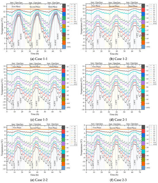
Figure 8.
The temperature variation in the wall in Section 1.
As outdoor temperatures gradually decreased, it took longer for the wall temperature to stabilize into periodic fluctuations, resulting in more pronounced temperature variations. Over time, as periodic fluctuations stabilized, the peak and trough temperatures of each point gradually increased. The peak and trough temperatures recorded at 24 h intervals were initially low but showed a gradual upward trend. The temperature amplitudes at 48 h were second only to those at 72 h. From the initial timepoint, temperatures began to decline, with the curves showing a downward trend. By 6 a.m., a gradual temperature increase was observed. Between 12 and 14 p.m., temperatures reached their peak, fluctuating within a narrow range of 1 °C, subsequently followed by a decrease. These temperatures fluctuated steadily and periodically, ranging from −15 °C to 15 °C. Based on observations from both indoor and outdoor environments under varying working conditions, it becomes evident that while the temperature change pattern of the walls in each group remains consistent, the magnitude of change differs, as does the time taken to reach the peak temperature, refer to Table 7.
Table 7.
Temperature Fluctuation Range at Measuring Points of Section 1 Under Varying Operational Conditions.
4.1.2. Temperature Variations in Section 2 Across Diverse Working Conditions
Figure 9a–f corresponds to the six working conditions outlined in Section 2. The temperature shifts exhibit irregular periodic patterns influenced by external temperature changes. The temperature waveforms at various points along the wall align with indoor and outdoor temperature fluctuations. Upon comparing temperatures across working conditions 1-1, 1-2, and 1-3, it is evident that the outermost surface node B1 of each condition displays periodic variations when compared to the central point B6 of the wall. However, these variations are significantly less pronounced than those observed at point B1, with the temperature amplitude progressively diminishing towards the center. As one moves closer to the wall’s interior, the surface temperature becomes increasingly insulated from external influences, resulting in a phase delay. As outdoor temperatures decline, so do the temperatures at points 1-1, 1-2, and 1-3 under these working conditions. In Figure 9a–c, the lowest temperature recorded at point B1 drops from −1 °C to −11.5 °C, while the highest temperature decreases from 10.5 °C to −1 °C. Similar trends are observed for points B2–B7, while point B8, located closest to the indoor side, remains relatively stable. Based on changes in the indoor and outdoor temperature and humidity environment under conditions 1-2, a gradual decrease in temperature is observed at each point for conditions 2-1, 2-2, and 2-3. Specifically, the lowest temperature at point B1 falls from −5 °C to −12 °C, and the highest temperature decreases from 2 °C to −2 °C. Similar patterns are seen at other points, while point B8, closest to the indoor side, experiences a temperature drop from 13 °C to 6 °C.
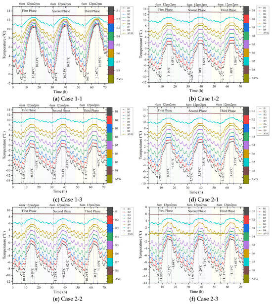
Figure 9.
The temperature variation in the wall in Section 2.
Table 8 presents the amplitude of the temperature variation at points across different working conditions. Upon comparing the temperature fluctuations within the walls of Sections 1 and 2 in Figure 9a–f, it is evident that Section 2 exhibits slightly smaller variations, indicating a more stable temperature profile. Upon comparing the temperatures of the various sections in Figure 9 and Figure 10, it is evident that the temperature at points B2–B8 of the Section 2 wall is notably higher than that at points A2–A8 of the Section 1 wall. Notable temperature differences are observed between points A1, A2, A4, and A5 as compared to B1, B2, B4, and B5. The significant temperature disparities between points B3, B4, B5, and B6 suggest that the prefabricated building joints notably affect the indoor and outdoor wall temperatures. This influence can potentially lead to an increased heat loss and more rapid temperature transfer in colder months. Points B1–B6 in Section 2’s wall show pronounced temperature fluctuations, aligning closely with outdoor temperature parameters. Notably, the temperature differences between points B6, B7, and B8 are substantial, with the temperatures at B6–B8 being notably lower than those at A6–A8 in Section 1’s wall. This finding underscores that the temperature gradient within the lightweight concrete wall is markedly reduced compared to the cast-in-place concrete wall. Opting for matrix materials with lower thermal conductivity can effectively minimize the temperature gradient disparity between the base wall and the insulation layer. This effect is primarily attributed to the cast-in-place pozzolan concrete’s significant thermal resistance. Temperature variations in Section 1 and 2 wall assemblies are presented in Figure 10.
Table 8.
Temperature Fluctuation Range at Measuring Points of Section 2 Under Varying Operational Conditions.
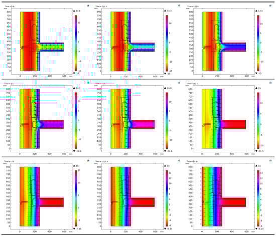
Figure 10.
Temperature variations in Section 1 and 2 wall assemblies.
4.2. Changes in Relative Humidity of Measuring Points in the Wall
4.2.1. Section 1 Variations in Relative Humidity Under Different Working Conditions
Figure 11 illustrates the relative humidity variations in the wall of Section 1 across different working conditions. The wall exhibits a rapid transition to a steady humidity state, indicating its entry into this phase. The moisture content within the wall tends to stabilize in accordance with the indoor and outdoor environmental parameters, undergoing periodic changes over time. During winter, the relative humidity of the wall primarily oscillates between 10% and 60%, with occasional spikes reaching 70%. These spikes are attributed to the instability of the initial calculation values, resulting in elevated relative humidity readings. Upon comparing the relative humidity of Section 1 in Figure 11a–f, it becomes evident that the periodic patterns of the moisture content variation within the wall are broadly similar, albeit with a general downward trend. As the wall reaches a normal state of heat and moisture transfer, measurement points closer to the outdoor environment are more significantly influenced, exhibiting more pronounced fluctuations in amplitude. Specifically, the relative humidity at point A1 on the wall’s exterior surface ranges from 3% to 70%. Points A2 (within the concrete layer) and A3 (at the interface between the concrete and insulation layers) experience relative humidity variations between 10% and 55%. Meanwhile, points A4 and A5, located within the insulation layer and the insulated lightweight concrete, respectively, show relative humidity changes within the 9% to 48% range.
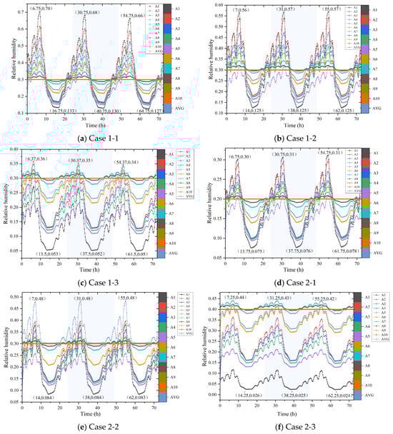
Figure 11.
Relative humidity change in Section 1 wall.
Upon comparing the working conditions depicted in Figure 11b 1-2 and Figure 11d 2-1, a similar underlying trend is evident. However, the relative humidity at each point within the wall under working conditions 1-2 surpasses that of working conditions 2-1, albeit with varying speeds and temperatures. Refer to Table 9 for the variation amplitude of the relative humidity at different points across various working conditions. As time progresses, water is continuously lost to the external environment, resulting in a gradual decrease in the overall relative humidity across all working conditions. This rate of decline, however, is slowly tapering off. Nonetheless, the peaks and troughs of the relative humidity fluctuate under different working conditions. Specifically, the peaks and troughs for working conditions 2-1 and 2-3 are slowly increasing, while those for 1-2 and 2-2 remain unchanged. The other working conditions, on the other hand, are gradually decreasing in line with the overall trend.
Table 9.
Relative Humidity Fluctuation Range at Measuring Points of Section 1 Wall Under Varying Operational Conditions.
Based on Figure 11, the change curves for working conditions 1-1, 1-2, 2-1, and 2-2 bear a resemblance, whereas the change trends for working conditions 1-3 and 2-3 share similarities. This similarity arises because the former conditions involve temperature variations primarily within the range from 0 °C to −15 °C, while the latter conditions entail temperature fluctuations between −20 °C and −30 °C. When outdoor temperatures hover between −20 °C and −30 °C, the outdoor relative humidity ranges from 60% to 70% and 30% to 40%. Notably, the maximum and minimum relative humidity for conditions 1-3 and 2-3 stand at 44% and 5%, respectively. Evidently, as depicted in Figure 11c,f, the overall relative humidity for both these conditions is notably lower compared to the other conditions. This significant reduction is primarily attributed to the severe winter environmental conditions in extremely cold regions. As temperatures drop to freezing points, any liquid water within the wall solidifies, leading to a decrease in relative humidity. However, as external temperatures rise above freezing during daytime, the ice within the wall’s porous medium melts, resulting in an increase in water. Over time, the wall’s interior experiences continuous drying, maintaining an overall downward trend in relative humidity.
4.2.2. Section 2 Variations in Relative Humidity Under Different Working Conditions
Figure 12 illustrates variations in the relative humidity within the wall of Section 2 across different working conditions. The rate at which the wet steady-state stage is reached mirrors that of Section 1. Relative humidity oscillates in accordance with changes in the indoor and outdoor temperature and humidity. The fluctuation range of the wall’s relative humidity remains consistent across all working conditions when compared to Section 1. Notably, the relative humidity in Section 2, specifically under working conditions 1-3 and 2-3 depicted in Figure 12c, surpasses that of Section 1. This suggests that under extremely cold conditions, Section 2’s wall has a lower ice content and superior insulation performance compared to Section 1. Upon comparing the relative humidity of the wall in Section 1 across Figure 12a–f, it is evident that the wall’s moisture content follows a similar periodic pattern. However, Section 2 exhibits a more rhythmic change in relative humidity, with a more stable humidity gradient between points and a more regular reduction trend. This indicates that the absence of connecting joints in Section 2 leads to variations in relative humidity at interfaces due to differing material properties. Conversely, the presence of assembly joints in Section 1 facilitates the circulation of the relative humidity and temperature at interfaces, resulting in overlapping changes that can compromise the wall performance. Furthermore, Figure 12 reveals that when the heat and moisture transfer within the wall stabilizes, the relative humidity of points closer to the indoor environment is lower, with decreasing fluctuations. Specifically, point B8 on the wall’s inner surface experiences relative humidity fluctuations in the 20–40% range. The variation amplitude of the relative humidity is significantly higher at point B2 in the outer concrete layer compared to point B8 at the split interface of the cast-in situ pozzolanic concrete lightweight concrete layer. Notably, the relative humidity changes at point B1 on the wall’s outer surface closely mirror outdoor relative humidity variations, highlighting the outer side’s susceptibility to external environmental influences.
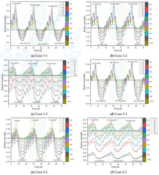
Figure 12.
Relative humidity change in Section 2 wall.
As Table 10 demonstrates, the relative humidity change value and peak valley value exhibit variations under different working conditions, with varying times to reach the peak valley. Influenced by the outdoor temperature, the relative humidity at point B1 on the external wall surface of Sections 1-1, 1-2, and 2-1 progressively increases under working conditions ranging from 0 °C to −10 °C. Conversely, the relative humidity at points B2, B3, and B4 located in the middle of the Section 2 wall experiences a sequential decrease. The relative humidity near the inner wall surface, at points B5, B6, and B7, undergoes diminishing changes, while the relative humidity at point B8 on the internal wall remains largely aligned with the set indoor relative humidity.
Table 10.
Relative Humidity Fluctuation Range at Measuring Points of Section 2 Wall Under Varying Operational Conditions.
Under working conditions 1-3, 2-2, and 2-3, where the external temperature ranges from −15 °C to −30 °C, the relative humidity at point B1 gradually decreases. In contrast, the relative humidity at the B2, B3, and B4 points in the middle of the Section 2 wall increases, surpassing that of B1 on the outer surface. The relative humidity at point B8, near the inner wall surface, mirrors the indoor relative humidity. Notably, the relative humidity change curve for working conditions 2-3 appears relatively smooth. This suggests that significant temperature fluctuations at the wall interface correspond to substantial humidity fluctuations. The temporal trend of relative humidity changes at points under various working conditions correlates with temperature changes at the same locations, indicating a strong influence of temperature variations on the distribution of the relative humidity within the wall. Relative humidity variations in Section 1 and 2 wall assemblies are provided in Figure 13.
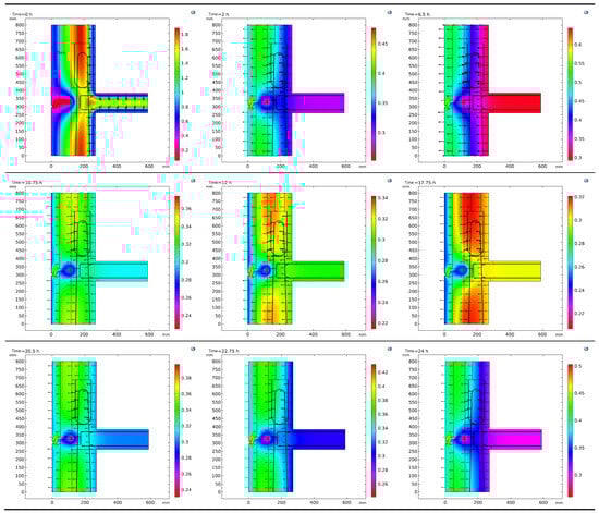
Figure 13.
Relative humidity variations in Section 1 and Section 2 wall assemblies.
4.3. Influence of Indoor and Outdoor Environment on Section 1 Wall
Figure 14 illustrates the variations in the temperature and relative humidity along the thickness direction of the wall in Section 1 under different working conditions. Specifically, Figure 14a depicts temperature shifts at various locations under these conditions, while Figure 14b represents relative humidity changes. The temperature distribution pattern from the outside to the inside is comparable across all working conditions, with temperatures progressively increasing from below zero. However, notable deviations are evident, particularly in working condition 1. Notably, the temperatures in working condition 1-1 consistently surpass those in other conditions, whereas working condition 2-3 exhibits the lowest temperatures with minimal fluctuations. As the set conditions alter, so do the temperatures associated with each working condition. The temperature distribution within the wall panel, particularly near the indoor side, mirrors the indoor temperature changes, albeit with a smaller variation amplitude compared to the wall panel’s interior surface. Conversely, the temperature distribution nearer to the outdoor side more closely follows the outdoor environmental temperature variations, with the external temperature exhibiting a smaller variation amplitude than the exterior surface. Furthermore, there is a minimal temperature variation within the 230–600 mm range, indicating that areas closer to the wall’s inner and outer surfaces are more susceptible to indoor and outdoor environmental temperature influences. Inside the wall, temperature transmissions are attenuated, resulting in minimal impacts from external temperature fluctuations.
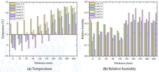
Figure 14.
Temperature and humidity changes in Section 1 wall.
Based on Figure 14b, the relative humidity exhibits a gradual decrease from 0 to 120 mm in thickness close to the outdoor side wall across all working conditions, subsequently rising to over 30% at 155–600 mm near the indoor side wall. As we move closer to the indoor side, there is a progressive drop in the relative humidity for each condition. Notably, at the former position, conditions 1-1 and 1-2 surpass other conditions, whereas at 155–600 mm, conditions 1-3, 2-2, and 2-3 prevail over conditions 1-1 and 1-2. The escalation in the moisture transfer leads to an augmentation in the latent heat transfer on the wall’s inner surface, causing the temperature of this surface to recommence its descent. The more pronounced the disparity between the internal and external humidity, the more evident the humidity increase becomes. Upon comparing temperature and humidity variations between working conditions 1-2 and 2-1, it is evident that, at a constant temperature, when the indoor and outdoor relative humidity of working condition 1-2 is reduced, the temperature of working condition 2-1 is marginally higher than that of 1-2 at the 0–155 mm wall thickness. However, both temperatures align closely at 155–600 mm, with the room relative humidity of working condition 1-2 persistently exceeding that of 2-1. Referring back to Figure 14b, the relative humidity at the insulation layer interface remains lower than within the concrete. Notably, under conditions 1-1 and 1-2, the internal relative humidity distributions mirror each other for both the insulation layer and the concrete, with the concrete consistently maintaining a higher moisture content than the insulation layer. This phenomenon is attributed to the concrete’s capacity to retain a significant amount of moisture absorbed from external sources. Across various working conditions, the moisture content on the outer surface exhibits substantial variation. As the thickness increases, the disparity in the relative humidity progressively narrows until the inner surface’s relative humidity aligns closely with the indoor relative humidity.
4.4. Influence of Indoor and Outdoor Environment on Section 2 Wall
Based on the analysis of Figure 14 and Figure 15, there is a distinct difference in the change trend of the relative humidity between Sections 1 and 2. Specifically, as the outdoor side wall thickness increases from 0 to 120 mm, the relative humidity of each working condition progressively rises. Conversely, it gradually decreases as the indoor side wall thickness increases from 120 to 600 mm. Within the wall thickness range from 50 to 270 mm, the relative humidity of working conditions 1-2 in Section 2 surpasses that of conditions 1-1. Similarly, the relative humidity of working conditions 2-3 in Section 2 is higher compared to Section 1. Notably, the lowest and highest values of relative humidity are observed at 0 and 155 mm, respectively, with the temperature being lower than that of Section 1. Furthermore, our findings indicate that the moisture content within the concrete wall primarily migrates from the center towards both sides. Although there is a slight increase in the temperature and relative humidity across all working conditions, the extent of this increase varies depending on the location. Notably, the rate of the relative humidity reduction at 155–270 mm in Section 2 is notably higher than that in Section 1.
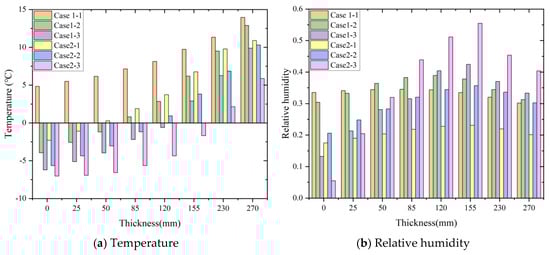
Figure 15.
Temperature and humidity changes in Section 2 wall.
Figure 15a illustrates the following: Under working condition 1-1, the temperature at various positions remains above 0 °C, with the relative humidity fluctuating between 30 and 34%. For conditions 1-2, the temperature at 0–50 mm is below 0 °C, gradually rising from the insulation layer to 13 °C. Here, the relative humidity ranges from 30 to 38%. In conditions 1-3, the temperature at 0–120 mm stands below 0 °C, increasing from 155 mm to 9.5 °C. The relative humidity varies between 14 and 42%. Under condition 2-1, the temperature at 0–25 mm is below 0 °C, progressively increasing from 25 mm to 11 °C. The relative humidity in this case fluctuates between 17 and 22%. In condition 2-2, the temperature at 0–85 mm is below 0 °C, rising from 120 mm to 10.5 °C. The relative humidity changes between 20 and 34%. Lastly, under conditions 2-3, the temperature at 0–155 mm is below 0 °C, gradually increasing from 230 mm to 7 °C. The relative humidity here fluctuates widely between 5 and 55%. Upon comparing conditions 2-3 with themselves, it is evident that an increase in the outdoor relative humidity not only reduces the temperature and heat storage capacity of the outdoor wall but also leads to unidirectional heat loss from the wall’s interior to the outside. This comparison highlights that the coupled heat and moisture transfer has a significantly greater impact on the temperature and humidity within the wall than on the internal surface temperature.
5. Conclusions
To investigate the phenomenon of wall connection joints freezing and thawing due to moisture transfer during winter, the established mathematical model was utilized to analyze the dynamic heat and moisture coupling transfer characteristics and patterns of the prefabricated concrete sandwich temperature-maintaining wall in Inner Mongolia under unstable environmental conditions. Furthermore, calculations and analyses were conducted to determine the time required for the wall to reach a stable moisture state, as well as the influencing factors, internal water content distribution, temperature distribution, and other variation characteristics and patterns under different operating conditions.
- (1)
- Under different working conditions, the fluctuation amplitude and waveform of the temperature and humidity within the wall exhibit periodic variations alongside changes in the outdoor temperature. As time progresses, the peak and valley values of the temperature at each point gradually increase, while the peak and valley values of the relative humidity gradually decrease. Notably, the change values and peak and valley values, as well as the time taken to reach the peak, differ between the two points. The closer one gets to the outer surface, the more pronounced the fluctuations in the temperature and humidity of the wall become. Conversely, as one approaches the inner surface wall, specifically near the A7 and A8 points, the temperature and humidity changes are relatively minor. The temperature and humidity at A9 and A10 remain largely unaffected, with a sequential decrease in the fluctuation amplitude, accompanied by hysteresis and attenuation.
- (2)
- The variation trend of the relative humidity over time aligns with temperature changes at different locations across various working conditions. Notably, the wall’s relative humidity curves differ in outdoor temperature ranges of 0–10 °C and −10–30 °C, highlighting a significant impact of wall temperature variations on relative humidity. When both indoor and outdoor temperatures remain constant, and only the relative humidity shifts, the fluctuation patterns are mostly consistent. However, under working conditions 1-2, the relative humidity is notably higher than under conditions 2-1, which is accompanied by variations in speed and temperature. As the outdoor temperature gradually approaches the freezing point, the liquid water within the wall freezes, resulting in a notable drop in the relative humidity for working conditions 1-3 and 2-3 compared to other scenarios. Over time, the wall’s internal relative humidity tends to decrease.
- (3)
- The variation curves of walls across different sections bear resemblances, yet the relative humidity gradient at each point of the wall in Section 2 exhibits greater stability. In comparison to Section 2, Section 1, which features joints, demonstrates a higher amplitude of temperature fluctuations. Consequently, the temperature disparities at various points along the wall are more pronounced, elevating the potential for indoor heat loss. This suggests that the presence of joint gaps facilitates a more rapid transfer of temperature and relative humidity between the material interfaces within the wall. Notably, the relative humidity at the insulation layer interface remains lower than that within the concrete interior. Furthermore, the temperature difference at the interface between the lightweight concrete wall and the cast-in-place concrete wall of Section 2 is more significant, while being lower in comparison to the cast-in-place concrete wall of Section 1. This indicates that the temperature gradient within the lightweight concrete wall is considerably less than that of the cast-in-place pozzolan concrete wall.
This study elucidates the frost formation mechanism influenced by joints in prefabricated components through a hygrothermally coupled numerical model, focusing on extreme low-temperature frosting scenarios while omitting hygrothermal transfer under high-temperature and high-humidity summer conditions. The current model employs a one-dimensional simplification, whereas practical engineering applications reveal microscopic surface irregularities and material anisotropy at prefabricated wall joint interfaces, potentially exacerbating localized condensation risks. Experimental investigations of the hygrothermal transfer across diverse connection nodes under real-world complex environments are therefore imperative.
Author Contributions
Conceptualization, L.H. and D.Z.; methodology, L.H. and D.Z.; software, L.H.; validation, L.H. and D.Z.; investigation, D.Z. and L.H.; writing—original draft preparation, L.H.; writing—review and editing, L.H. and D.Z.; visualization, L.H.; supervision, D.Z. and L.H.; funding acquisition, D.Z. All authors have read and agreed to the published version of the manuscript.
Funding
This project is supported by the National Natural Science Foundation of China, Project name: Carbon Footprint Analysis and Carbon Reduction Design Strategies for the Whole Life Cycle of Walls of Assembled Buildings in Inner Mongolia Region (Grant No.: 52168007); it is also supported by the Basic Scientific Research Business Expenses of Universities Directly under Inner Mongolia Autonomous Region, Project Name: Research on Carbon Reduction Design of Prefabricated Buildings in Inner Mongolia Based on Digital Twin Technology (Grant No.: JY20230053); Inner Mongolia Natural Science Foundation Project, Project Name: Small- and Medium-sized Public Buildings in Inner Mongolia Based on Digital Twin Technology Carbon Footprint Study (Grant No.: 2023LHMS05026); and the construction system and key technology of grassland human settlement environment (Grant No.: YLXKZX-NGD-004).
Data Availability Statement
The data presented in this study are available on request from the corresponding author.
Conflicts of Interest
The authors declare no conflicts of interest.
Nomenclature
| Notation list | |
| ma | The phase α (v, l. i) quality, kg, |
| The density of the phase α in Rev, (kg/m3) | |
| Natural density of phase α (kg/m3) | |
| Volumetric content in porous media (m3/m3) | |
| Flow rate of phase , kg/(m2·s) | |
| Liquid water transfer rate, expressed in kg/(m2∙s) | |
| Water vapor transfer rate, expressed in kg/(m2∙s) | |
| The rate of phase transition generation for the inner phase of Rev, kg/(m3·s) | |
| The internal energy density in REV, (J/m3) | |
| The specific internal energy of wet air, (J/kg) | |
| Specific internal energy of phase (J/kg) | |
| The mass concentrations of dry air in the gas phase, (kg/kg) | |
| The mass concentration of water vapor in the gas phase, (kg/kg) | |
| The convective flux of the gas phase, kg/(m2∙s) | |
| Wall thickness (m) | |
| Time (s) | |
| Temperature (K) | |
| Conductivity of liquid water (s0) | |
| Liquid water pressure (Pa) | |
| Partial pressure of water vapor (Pa) | |
| Diffusivity of water vapor in free air (m2·s) | |
| Vapor gas constant, J/(kg·K) | |
| Diffusion resistance coefficient of water vapor | |
| Volume fraction of the gas phase (m3/m3) | |
| n | Porosity |
| Density (kg/m3) | |
| The thermal conduction heat flow (W/m2) | |
| Mass of liquid water and solid ice in the porous material (kg) | |
| The internal heat source term, (W/m3) | |
| Air phase | |
| Specific enthalpy of water vapor liquefaction (J/kg) | |
| Specific enthalpy of liquid water (J/kg) | |
| Greek symbols | |
| Sum of quantities | |
| ∇ | Differential operator |
| Subscripts | |
| i | Indoor |
| e | Outdoor |
| Wall surface | |
| Environment | |
References
- Wan, J.; Yu, S.; Wei, J. Effect of air layer on the coupled heat, air, and moisture transfer performance of multi-storey walls. Energy Sav. 2023, 42, 6–10. [Google Scholar]
- Fang, A.M.; Chen, Y.M.; Wu, L. Modeling and numerical investigation for hygrothermal behavior of porous building envelope subjected to the wind driven rain. Energy Build. 2021, 231, 110572. [Google Scholar] [CrossRef]
- Hou, S.; Liu, F.; Wang, S.; Bian, H. Coupled heat and moisture transfer in hollow concrete block wall filled with compressed straw bricks. Energy Build. 2017, 135, 74–84. [Google Scholar] [CrossRef]
- Chen, Y.; Mao, C.; Chen, G.; He, Y. Impact of Moisture Migration on Heat Transfer Performance at Vertical Joints of ‘One-Line’ Sandwich Insulation Composite Exterior Walls. Buildings 2025, 15, 1084. [Google Scholar] [CrossRef]
- Yang, Y.T. Study on Coupled Heat and Moisture Transfer Characteristics of Prefabricated ECC Sandwich Composite Exterior Wall Panels. Master’s Thesis, China University of Mining and Technology, Xuzhou, China, 2021. [Google Scholar]
- Ji, J.J. Research on the Influence of Prefabricated Building Connectors on Hygrothermal Performance and Building Energy Consumption of Exterior Walls. Master’s Thesis, Nanchang University, Nanchang, China, 2022. [Google Scholar]
- Zhao, G.Q.; Chen, W.Q.; Zhao, D.P.; Li, K. Mechanical Properties of Prefabricated Cold-Formed Steel Stud Wall Panels Sheathed with Fireproof Phenolic Boards under Out-of-Plane Loading. Buildings 2022, 12, 897. [Google Scholar] [CrossRef]
- Call, W.C.M. Thermal properties of sandwich panels. Concr. Int. Design Constr. 1985, 7, 34–41. [Google Scholar]
- Kraus, M. Hygrothermal Analysis of Indoor Environment of Residential Prefabricated Buildings: World Multidisciplinary Civil Engineering-Architecture-Urban Planning Symposium-WMCAUS. World Multidisciplinary Civil Engineering-Architecture-Urban Planning Symposium (WMCAUS). IOP Conf. Ser. Mater. Sci. Eng. 2017, 245, 042071. [Google Scholar]
- Xue, Y.C.; Fan, Y.F.; Chen, S.Q.; Wang, Z.; Gao, W.; Sun, Z.; Ge, J. Heat and moisture transfer in wall-to-floor thermal bridges and its influence on thermal performance. Energy Build. 2023, 279, 112642. [Google Scholar] [CrossRef]
- Philip, J.R.; DeVries, D.A. Moisture movement in porous materials under temperaturegradients. Trans. Am. Geophys. Union 1958, 38, 222–232. [Google Scholar]
- Künzel, H.M.; Holm, A.; Zirkelbach, D.; Karagiozis, A.N. Simulation of Indoor Temperature and Humidity Conditions Including Hygrothermal Interactions with the Building Envelope; Elsevier Ltd.: Amsterdam, The Netherlands, 2004; Volume 78, pp. 554–561. [Google Scholar]
- Feng, C. An Examination of the Driving Potential of Water Transfer in Building Envelopes. Build. Energy Effic. 2022, 50, 1–7. [Google Scholar]
- Wang, Y.Y.; Liu, K.; Tian, Y.; Fan, Y.; Liu, Y. The effect of moisture transfer on heat transfer of roof-wall corner hygrothermal bridge structure. Indoor Built Environ. 2023, 32, 881–901. [Google Scholar] [CrossRef]
- Dong, W.Q.; Chen, Y.M.; Bao, Y.; Fang, A. A validation of dynamic hygrothermal model with coupled heat and moisture transfer in porous building materials and envelopes. J. Build. Eng. 2020, 32, 101484. [Google Scholar] [CrossRef]
- Qin, M.; Belarbi, R.; Aït-Mokhtar, A.; Nilsson, L.-O. Coupled heat and moisture transfer in multi-layer building materials. Constr. Build. Mater. 2009, 23, 967–975. [Google Scholar] [CrossRef]
- Liu, R.; Huang, Y.W. Heat and Moisture Transfer Characteristics of Multilayer Walls: Cleaner Energy for Cleaner Cities. Energy Procedia 2018, 152, 324–329. [Google Scholar]
- Bagaric, M.; Pecur, I.B.; Milovanovic, B. Hygrothermal performance of ventilated prefabricated sandwich wall panel from recycled construction and demolition waste—A case study. Energy Build. 2020, 206, 109573. [Google Scholar] [CrossRef]
- Li, H.P.; Yang, S.Y.; Zha, Z.Q.; Fei, B.; Wang, X. Hygrothermal Properties Analysis of Bamboo Building Envelope with Different Insulation Systems in Five Climate Zones. Buildings 2023, 13, 1214. [Google Scholar] [CrossRef]
- Cai, S.; Xia, L.; Xu, H.; Li, X.; Liu, Z.; Cremaschi, L. Effect of internal structure on dynamically coupled heat and moisture transfer in closed-cell thermal insulation. Int. J. Heat Mass Transf. 2022, 185, 122391. [Google Scholar] [CrossRef]
- Matsumoto, M.; Hokoi, S.; Hatano, M. Model for simulation of freezing and thawing processes in building materials. Build. Environ. 2001, 36, 733–742. [Google Scholar] [CrossRef]
- Kong, F.H.; Zhang, Q.L. Effect of heat and mass coupled transfer combined with freezing process on building exterior envelope. Energy Build. 2013, 62, 486–495. [Google Scholar] [CrossRef]
- Wang, Y.; Wang, Q.; Chen, R.F.; Zhang, C.; Song, J. Comparative analysis on heat and moisture transfer of composite insulation walls. Int. J. Low-Carbon Technol. 2024, 19, 2108–2118. [Google Scholar] [CrossRef]
- Shen, X.W.; Li, L.J.; Cui, W.Z.; Feng, Y. Thermal and moisture performance of external thermal insulation system with periodic freezing-thawing. Appl. Therm. Eng. 2020, 181, 115920. [Google Scholar] [CrossRef]
- Wu, W.Y. Fluid Mechanics Volume I; Peking University Press: Beijing, China, 1982. [Google Scholar]
- BS EN15026: 2007; Hygrothermal Performance of Building Components and Buildingelements: Assessment of Moisture Transfer by Numerical Simulation. BSI: London, UK, 2007.
- Gao, W.; Dong, X.; Zheng, Y. Preliminary Report on the Properties of Volcanic Slag and Volcanic Slag Concrete Materials in Ximeng, Inner Mongolia. J. Hebei Norm. Univ. Sci. Technol. 2007, 4, 46–49. [Google Scholar]
Disclaimer/Publisher’s Note: The statements, opinions and data contained in all publications are solely those of the individual author(s) and contributor(s) and not of MDPI and/or the editor(s). MDPI and/or the editor(s) disclaim responsibility for any injury to people or property resulting from any ideas, methods, instructions or products referred to in the content. |
© 2025 by the authors. Licensee MDPI, Basel, Switzerland. This article is an open access article distributed under the terms and conditions of the Creative Commons Attribution (CC BY) license (https://creativecommons.org/licenses/by/4.0/).