Abstract
The outdoor environment greatly affects indoor thermal conditions, yet few investigations have been carried out to optimize the outdoor environment physical parameters that lead to improvements in the indoor thermal environment. This paper proposes a method to optimize the pavement albedo, greening rate, and the neighboring building distance for an office building in Shanghai, to improve its indoor thermal conditions and energy performance. Firstly, the Latin hypercube sampling approach was applied to obtain 68 sets of design samples. Secondly, ENVI-met 5.1 coupled with EnergyPlus 23.1.0 was adopted to perform simulations and obtain the discomfort degree hours and building energy consumption. Thirdly, two machine learning prediction algorithms were used to develop discomfort degree hours and energy consumption models, and the artificial neural network models were found to have better prediction performance with R-squares greater than 0.99. Fourthly, the artificial neural network models were used as fitness functions for seven optimization algorithms and Pareto front solutions were obtained during the optimization process. The optimal solutions help to reduce building energy consumption by up to 4.12% and indoor discomfort degree hours by up to 7.45%, as against the reference building. This study contributes to multi-objective outdoor physical design optimization for the indoor thermal environment, comparative analysis of prediction models, and optimization approaches.
1. Introduction
The outdoor neighboring environment greatly affects indoor thermal conditions such as indoor air temperature (IAT), air pollution, and energy performance. Typical outdoor environment parameters include key features of surrounding buildings, greenery, road surface, sky view, and water bodies [1].
The impact of the distance between surrounding buildings and the targeted building (DSBTB) is often expressed as the building height to street width (H/W) ratio. It affects the solar radiation absorbed by the building envelope, and thus the building energy performance. Its impact on cooling and heating energy needs might vary in different climate conditions [2]. For example, it was found that in the oceanic climate zone of Copenhagen, an increase in H/W ratio leads to reduced cooling demand and increased heating demand by allowing less incident solar radiation to enter the building [3]. In the hot desert climate of Phoenix, an increased H/W ratio leads to reduced cooling and energy demand [4]. Increased H/W ratio leads to reduced cooling demand in all the cities in the hot summer and cold winter (HSCW) region in China. However, heating energy needs increased in two cities (Shanghai and Wuhan) while there was virtually no difference in the other three cities (Changsha, Chengdu, and Chongqing) as they received almost no solar radiation during the heating period [5]. Some researchers found that when H/W < 1, an increased H/W ratio leads to slightly increased cooling energy needs and slightly decreased heating energy needs, and when H/W > 1, an increased H/W ratio leads to sharply decreased cooling and decreased heating energy needs in the predominantly humid continental climate of Boston. Some researchers found that H/W ratio has no impact of on heating energy needs unless it is higher than 0.52 [6]. However, those studies primarily focus on the impact of H/W ratio on building energy performance without considering other outdoor design physical parameters.
Greening provides shading for the building. Researchers often employed numerical simulations such as ENVI-met to evaluate how greening affects indoor thermal conditions. Greening was found to reduce indoor temperature by 0.6–1.5 °C, and increase the monthly average indoor relative humidity by 0.9–3.5% [7]. Taleghani et al. [8] found that a 17% increase in tree cover rate could lower the temperature by 1.1 °C during the hottest time of day at a university campus in Manchester. Some researchers found that the shading effect of greening leads to increased cooling load and decreased heating load [9]. Some other researchers found that planting trees along different directions of the building has different impacts on building thermal loads, e.g., cooling load is largely affected by planting trees along the west wall while heating load is largely affected by planting trees along the north wall. Tree species also affect the indoor thermal conditions. Deciduous trees obstruct solar beam, reduce indoor temperatures in summer, and transmit sunlight in winter, thus reducing both indoor cooling and heating needs [10]. Some researchers also found that an increased greening rate reduces overall building energy consumption [11], and cooling and energy needs [12]. However, those studies primarily focus on the greening effect without considering other outdoor design physical parameters.
The pavement albedo also affects the indoor thermal conditions. On one hand, high pavement albedo leads to significantly reduced road surface and outdoor air temperature (OAT), which leads to reduced cooling energy demand and increased heating energy demand [13,14,15]. On the other hand, certain amount of road surface-reflected solar radiation will be absorbed by the exterior wall of the building, which will cause the indoor temperature to increase [16]. Many studies have confirmed that high-albedo pavement can reduce cooling energy needs in summer [14,15,17,18]. For example, results from TRNSYS simulation demonstrated peak cooling demand reduction of 7.8–10.2% by replacing black asphalt with gray asphalt [14]; high-albedo concrete leads to 0.2–2.5% cooling energy reduction in Cairo [15]; an increase in albedo from 0.1 to 0.6 leads to the maximum temperature reduction of 0.4–1.4 °C. However, some other researchers have come to the opposite conclusion [4,19,20]. They found that the higher the albedo of the pavement, the greater its ability to reflect solar radiation, leading to higher surrounding building surface temperatures and cooling energy needs. Further studies found a close relationship between pavement albedo and H/W ratio. For example, in urban canyons with high H/W ratios, deep/narrow urban canyons prevent a large proportion of shortwave radiation from reaching the ground, which weakens the effects of pavement reflectivity on indoor thermal conditions [4]. Only when H/W < 1 can solar radiation be largely reflected by the road surface and effectively change the urban albedo [4,21]. When H/W is small, increased road surface albedo leads to a reduced cooling load; however, the cooling load starts to rise when H/W increases to a threshold [19]. Current studies mainly focused on pavement’s effect in summer, and only a few articles investigated its effect in winter and pointed out that the cooling effect of pavement may cause thermal discomfort and increased heating energy consumption in winter [22]. Moreover, the road surface’s effects on the indoor thermal conditions could be very small in certain areas [15], which requires combining high-albedo materials with greenery to magnify its effects. Few researchers have taken into account the impact of the distance between surrounding buildings and the target building, the greening factor, and pavement albedo together.
Recent studies also evaluate the impact of other factors on the indoor environment, e.g., layout, block form, and model scale. Wang and Zhang [23] investigated the impact of subway entrance layout on pollutant transportation to the indoors and found severe indoor pollution at the windward side subway entrances. Du et al. [24] evaluated the impact of block form on building energy consumption and revealed that deep learning models combined with machine learning algorithms can achieve a prediction accuracy of up to 98.3% in building energy consumption. Gonçalves et al. [25] performed multiscale modeling to predict the thermal performance of naturally ventilated social housing in northern Brazil and found that building thermal performance is highly affected by climate change.
Many scholars have investigated on how to improve the building energy performance and indoor thermal comfort through multi-objective optimization. However, they either focus on building envelope [26,27], heating, ventilation, and air-conditioning (HVAC) system control [28], or a combination of the two sets of parameters and not the outdoor design parameters [29], or power generation [30]. Meanwhile, prediction models were often developed for quick calculation of the objective function, based on building envelope design parameters [26,27] or HVAC system control parameters [28], or their combinations [29]. A few scholars have developed prediction models on the relationship between outdoor and indoor environment. For example, Liu et al. [2] developed a support vector regression (SVR) model to predict the impact of shading from surrounding buildings on heating/cooling energy demands using building morphology, block form, geographical information, and climate characteristics with 95% of the relative errors falling within the range of −5.78–7.71%. Deng et al. [6] used a multiple linear regression (MLR) model to evaluate the impact of residential cluster layout on building heating energy consumption. Xu et al. [20] evaluated the performances of different machine learning models on the relationship between pavement albedo and building energy demand and the neural network model was found to have the best performance. However, those prediction models were not applied for design optimization purposes.
The above literature survey shows that: (1) most studies focus on individual outdoor physical environmental parameters; (2) current studies mainly focused on the impact of pavement in summer and not in winter; (3) sensitivity analysis rather than optimization was performed; (4) few investigations focused on optimizing multiple outdoor parameters to improve indoor thermal energy performance; (5) although there are a few prediction models on the relationship between outdoor physical design parameters on indoor thermal and energy performance, they were not applied for design optimization. Meanwhile, no model on the relationship between the surrounding buildings, greening rate, pavement albedo, and indoor discomfort degree hours (IDDHs) and building energy consumption (BEC) has been found.
To fill the research gaps, this article attempts to optimize multiple outdoor design parameters, i.e., surrounding buildings, greening rate, and pavement albedo, to reduce indoor thermal discomfort and improve building energy performance. Specifically, a building and its surrounding environment, located in the hot summer and cold winter area in Shanghai, China, were selected. The building and surrounding environment were modeled by coupling ENVI-met and EnergyPlus to obtain microclimate conditions, indoor discomfort degree hours (IDDHs), and building energy consumption (BEC) on a representative summer day and a representative winter day. A Latin Hypercube Sampling (LHS) approach was applied to create the design database and obtain the associated IDDHs and BEC of the samples. Two machine learning (ML) approaches were applied for IDDHs and BEC prediction model development based on outdoor design parameters, and the better prediction models were selected to serve as fitness functions for seven optimization algorithms and Pareto solutions were obtained during the optimization process. Recommendations on outdoor physical environmental parameters are provided at the end of the paper. The key innovation of this study is a four-step framework that enables multi-objective optimization of multiple outdoor physical design parameters, aiming to improve indoor thermal environments and energy performance while providing guidance for urban planning practitioners.
2. Method
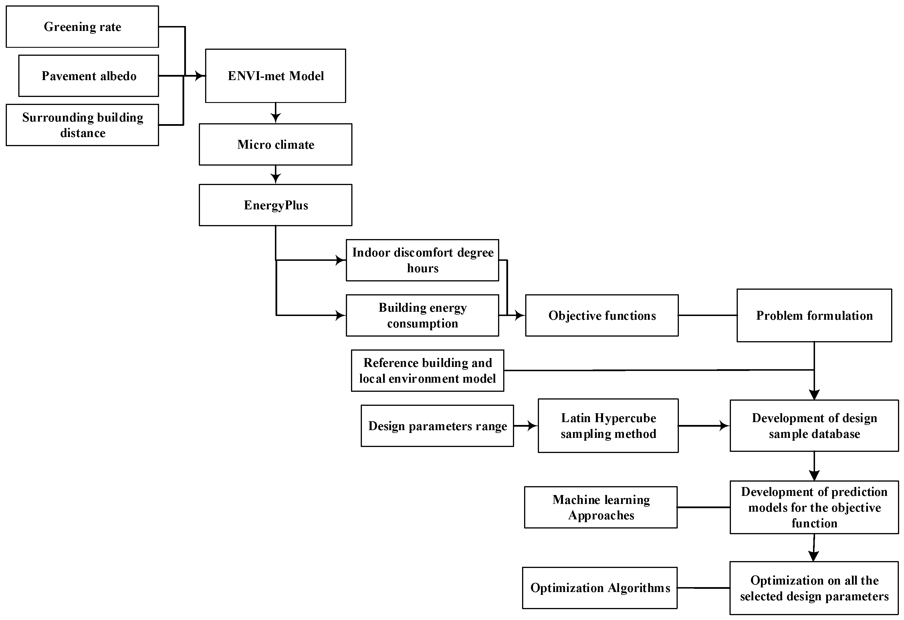
A four-step research framework was applied (Figure 1). The first step was problem formulation, where the values of the objective functions were computed by coupling the simulations of ENVI-met with EnergyPlus. The coupled simulation of ENVI-met and EnergyPlus is a one-way process [1]. The outcomes of micro-climate data from ENVI-met simulation were used as meteorological data in the EnergyPlus program to perform building simulation. The micro-climate data include temperature, relative humidity, wind speed, and wind direction around the target building from 9:00 on January 20 to 24:00 on 21 January and from 9:00 on July 20 to 24:00 on 21 July. These microclimate data were used to replace the corresponding data in the meteorological data file from the EnergyPlus official website, and then used as the inputs for the EnergyPlus program. Finally, the indoor temperature and energy consumption were obtained through the building simulation performed by EnergyPlus. In the second step, a design sample database was created using LHS technology. The third step involved the application of two ML approaches for prediction model development and employing the models to calculate the objective functions values. The last step involved coupling prediction models with optimization algorithms to perform optimization on all the selected design parameters.
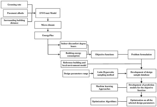
Figure 1.
Framework of the research method.
2.1. Objective Functions
The IDDHs and BEC were used as objective functions for optimization, which are described as:
where f1 is the IDDHs, in °C∙h; f2 is the BEC, in kWh.
The IDDHs can be obtained by [27]:
where IC is the cooling discomfort degree hours (CDDHs) and IH is the heating discomfort degree hours (HDDHs), in °C∙h.
The CDDHs and HDDHs can be calculated using Equations (3) and (4).
where is the IAT at time i, tH and tL are the higher and lower thermal comfort temperature limits, taken as 26 °C and 18 °C, respectively, according to JGJ 134-2010 [31]. The IAT was obtained by simulation through coupling ENVI-met with EnergyPlus.
2.2. Design Parameters and Ranges
The road pavement albedo, the greening rate, and the DSBTB were selected based on the literature survey. The lowest albedo from the pavement materials was found to be 0.04. According to Salvati et al. [16], when the albedo of the pavement is higher than 0.5, it will cause glare and reduce indoor visual comfort. Therefore, the pavement albedo was set to be 0.04~0.5.
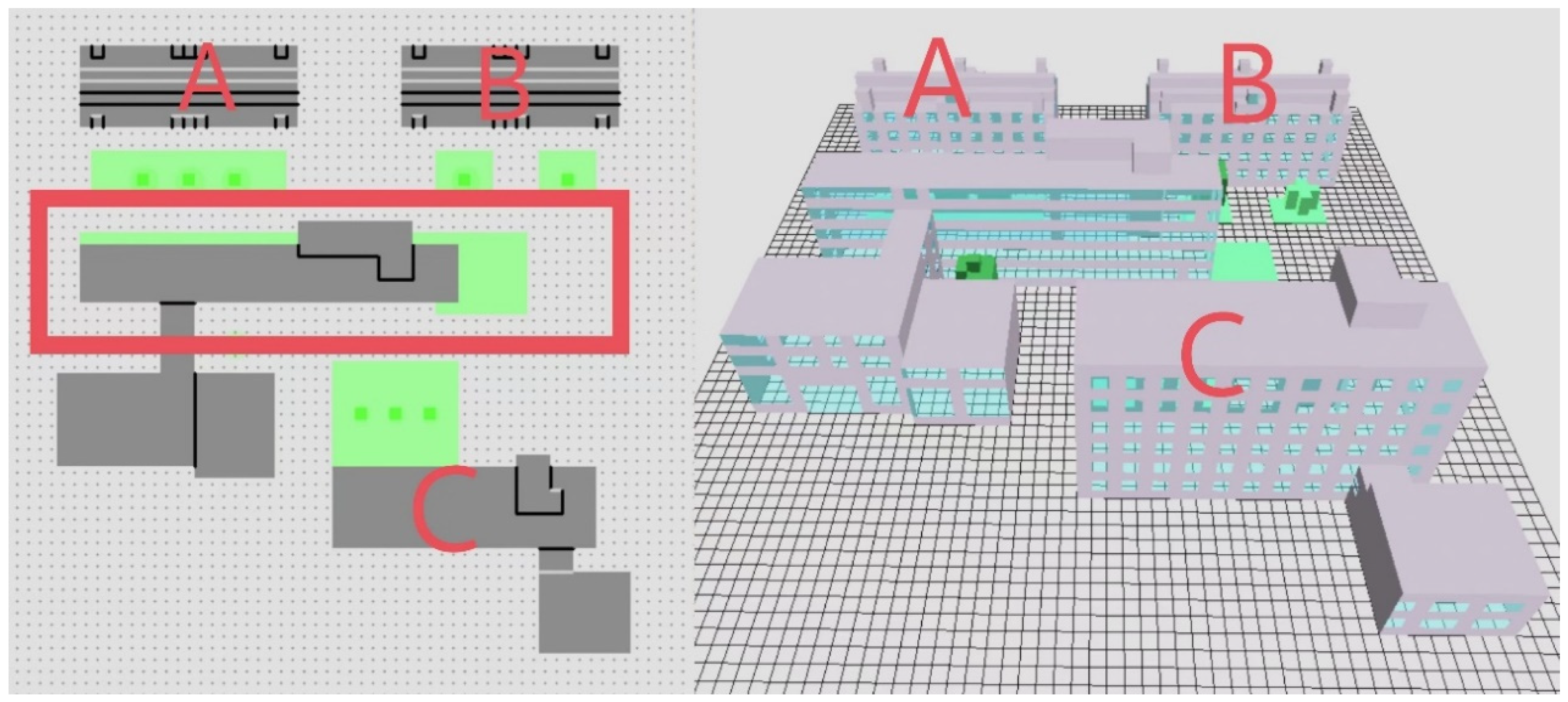
Figure 2 demonstrates the plan view of the ENVI-met model. Evergreen trees with a crown size of 5 m, a height of 11 m, and an average transmittance of 0.3 were selected. The trees were evenly arranged on the south/north side of the target building. The greening rate was calculated as the tree shadow area divided by the red box area. In order to leave enough space for roads, the greening rate was in the range of 3.7~15.4%, with 3.7% as the reference model.

Figure 2.
Plan view of the building under the ENVI-met environment, with the target building located in the red box.
To study the effects of the surrounding building distance, it was assumed that building A, B, and C could move along the south and north directions of the target building. In this study, the moving distance is set to be 0~8 m from their original positions.
Table 1 lists the values of the target building and the ranges of the investigated parameters.

Table 1.
Values of the target building and ranges of the parameters.
The target office building is in a university campus in Shanghai, in the HSCW region of China, with a yearly average temperature of 16.2 °C. The heating and cooling degree days of Shanghai are 1540 °C∙d, and 199 °C∙d, respectively. 21 July and 21 January were selected as representative days to evaluate the effects of multiple outdoor physical factors on the indoor thermal conditions.
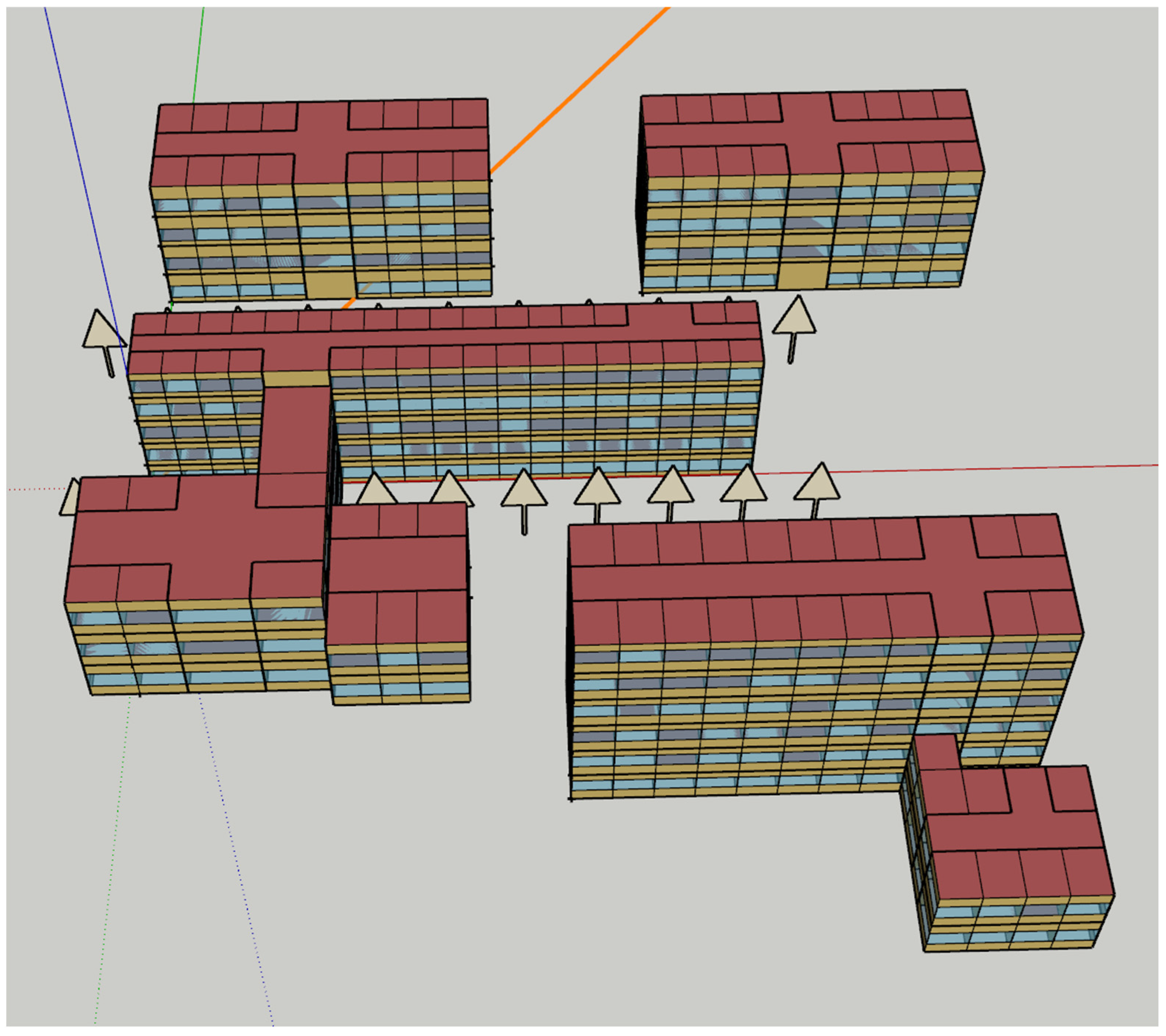
Figure 3 presents the plan view of the target building model (the one in the red box of Figure 1). According to the building standard, GB55015-2021 [32], the lighting power densities in the office room, in the corridor, and equipment power density were assigned as 6 W/m2, 2 W/m2, and 15 W/m2, respectively. The clothing insulation values were 0.5 clo in summer and 1.0 clo in winter and the occupancy density was assigned as 10 m2/person. The air change rate was assigned as 1 air change rate per hour (ACH). Except for the non-air-conditioned corridors and bathrooms, each room was configured with one split air conditioner. The summer and winter indoor temperature setpoints were assigned as 26 °C and 18 °C, respectively. In the EnergyPlus model, the trees are simplified as combinations of triangles and columns [33]. Table 2 lists the physical properties of the target building.

Figure 3.
The EnergyPlus building model, with the target building surrounded by trees.
Table 2.
Physical properties of the target building.
Table 3 lists the boundary conditions of the ENVI-met model.
Table 3.
Boundary conditions of the ENVI-met model.
The total IDDHs and BEC of the reference building on the two typical days were 100.79 °C∙h and 2091.29 kWh, respectively.
2.3. Prediction Model
2.3.1. Sample Database Generation
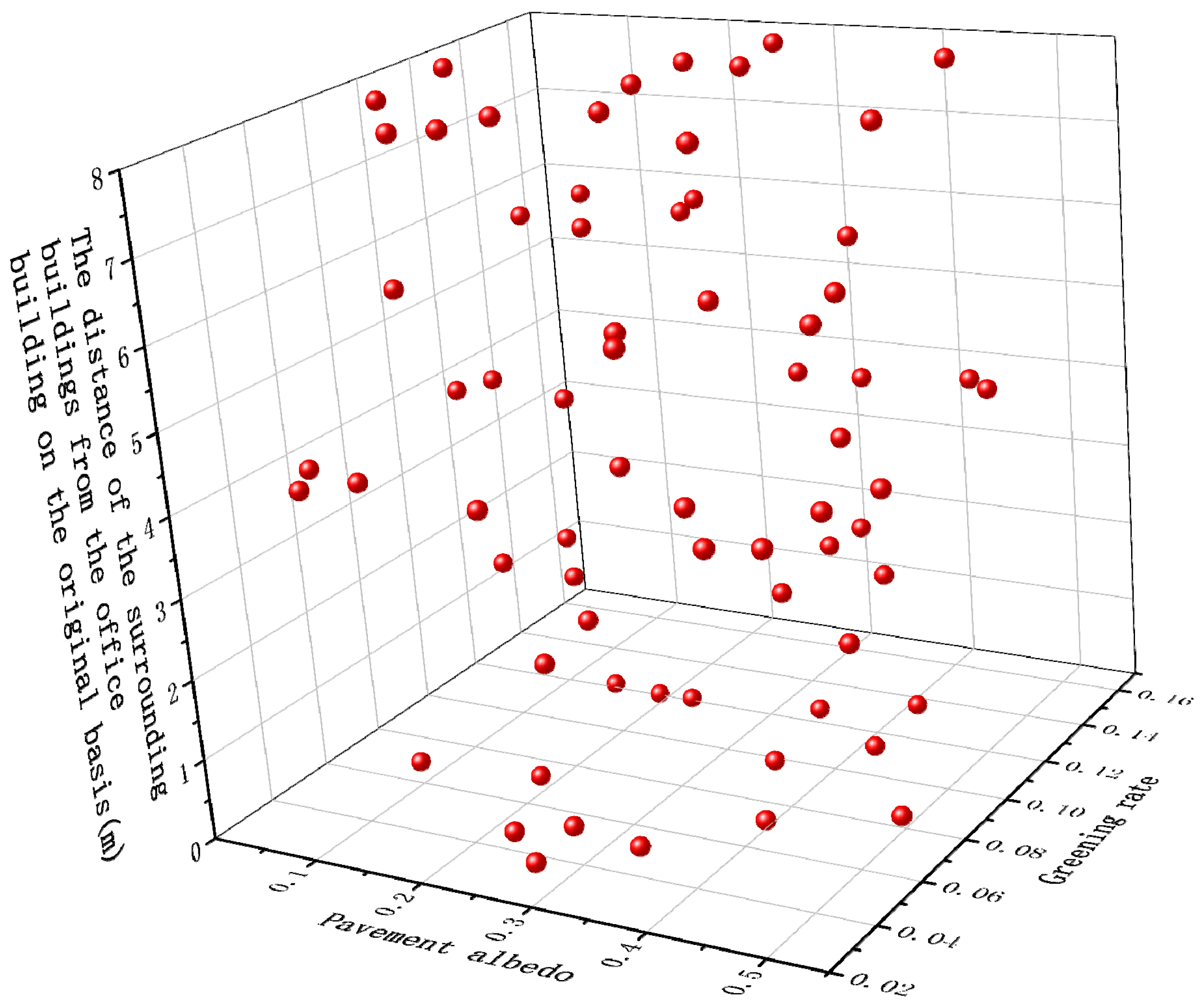
The LHS method was applied to generate the sample database to ensure even distribution over the multiple-dimensional space. Samples were extracted from each evenly divided segment of the sample space, requiring fewer samples while making them more representative compared to the Monte Carlo sampling approach [34]. The number of samples was determined according to N ≥ 22.5 × M, with N being the sample size, and M being the number of variables, which can accurately sample the search space [35]. A total of 68 samples were generated. Figure 4 presents a visualization of the sample distribution.

Figure 4.
Visualization of sample distribution.
2.3.2. Prediction Model Development
Two data-driven approaches, an artificial neural network and locally weighted regression, were applied for IDDHs and BEC prediction model development.
- Artificial neural network model
An Artificial Neural Network (ANN) learns the response of biological neurons to handle the information flow. It is effective in predicting BEC [36] and IAT [37,38] based on outdoor environmental conditions. It consists of three layers, i.e., input, hidden, and output layers. The number of nodes of the hidden layer can usually be obtained as:
where m, a, and b are the numbers of nodes of the input layer, input variables, and output variables, respectively. c is a constant in the range 0~10.
A backpropagation neural network (BPNN) was adopted. It was proposed by Rumelhart et al. [39], with wide application. The road pavement albedo, greening rate, and the DSBTB were the inputs, and IDDHs and BEC are the outputs of the BPNN model. Table 4 presents the settings of the BPNN model.
Table 4.
Settings of the BPNN model.
- Locally Weighted Regression
Locally weighted regression (LWR) utilizes a multi-variable smoothing procedure to fit the regression surface [40]. The function of the independent variables was locally fitted using the weighted least square method in a moving fashion analogous to time series moving average computation. Unlike other prediction models, such as BPNN models, linear regression models, etc., LWR cannot generate a single functional relationship. New regression coefficients need to be obtained by fitting based on existing training samples for each new sample to be predicted.
The Gaussian kernel function was employed as the weight function in this study. It can be expressed as:
where W is the Gaussian kernel function; k is the rate at which the weight changes with distance. k value increases with reduced speed on the decrease in the weight.
The regression coefficient could be obtained as:
In this study, the independent variable X represents the road pavement albedo, greening rate, and the DSBTB; the dependent variables represent IDDHs and BEC. The best ratio of testing vs. training was found to be 20:80.
2.4. Optimization Algorithm
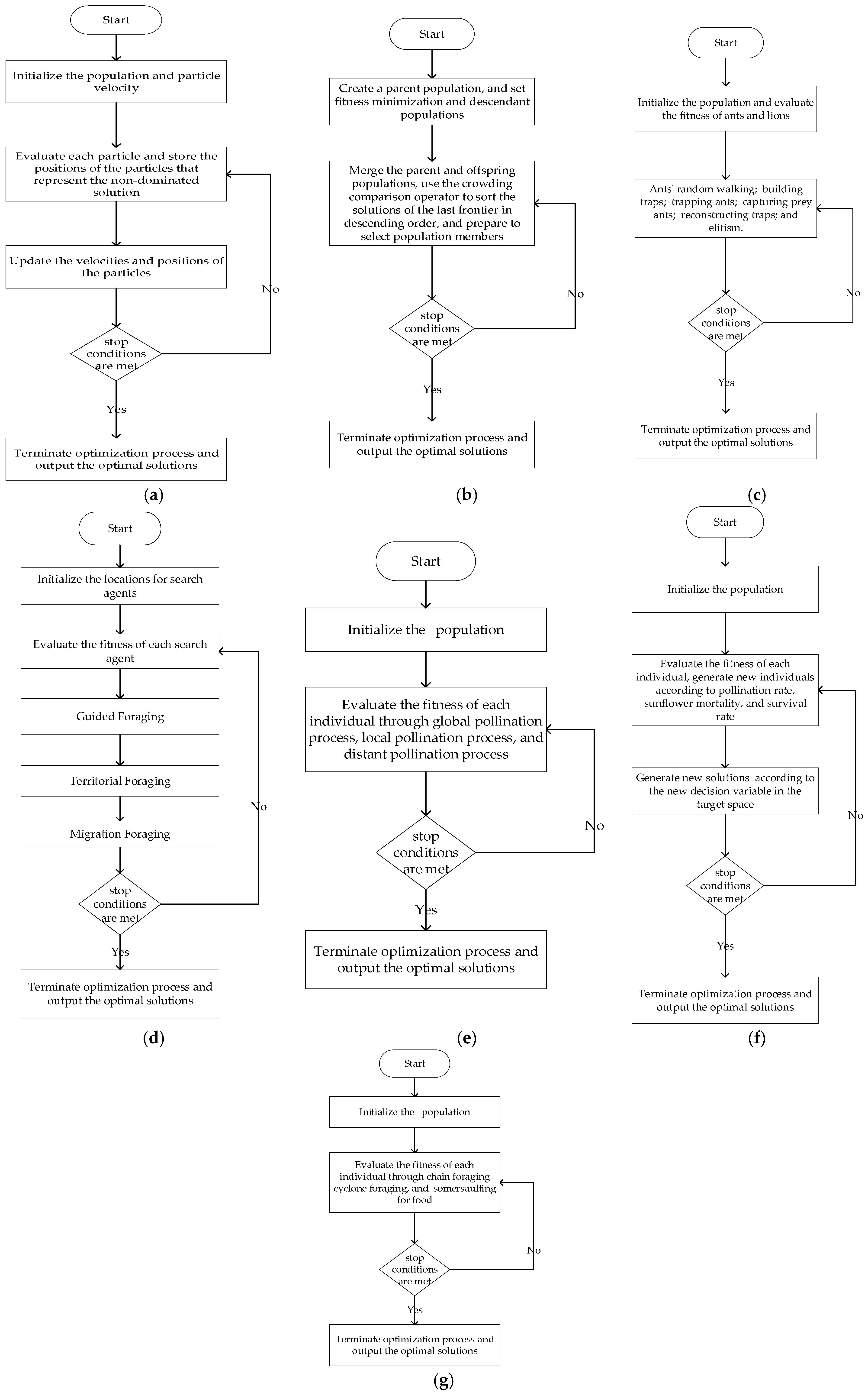
Seven optimization algorithms, which have been tested in other applications, were selected to couple with the prediction models to find the optimal solutions of outdoor design parameters to improve the thermal performance of the building. These algorithms have their own unique features in solving multi-objective optimization problems. The optimal solution outcomes of these algorithms were compared to find the best ones suitable for this study. Figure 5 presents the flow charts for each optimization algorithm.
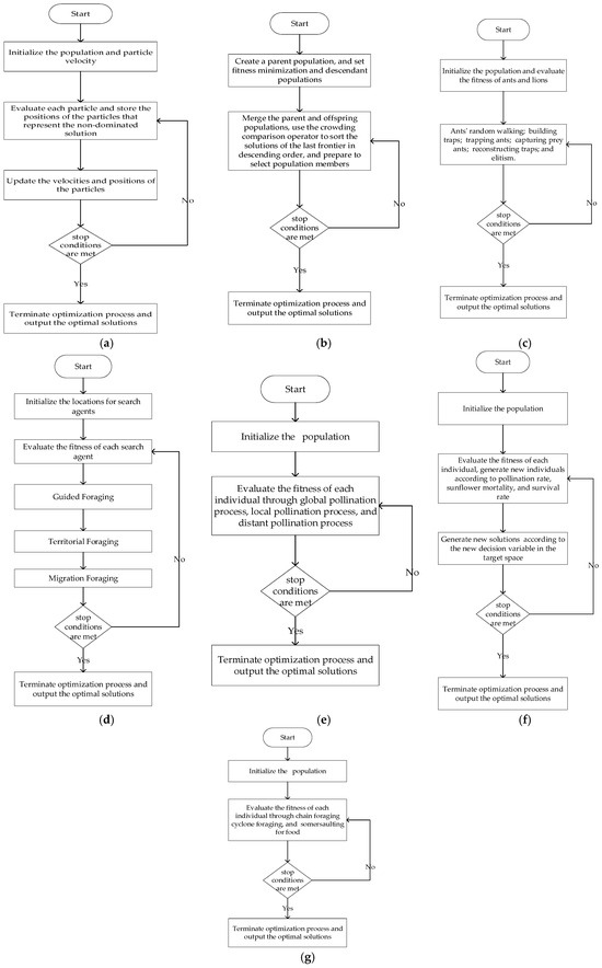
Figure 5.
Flow chart of each optimization algorithm. (a) MOPSO; (b) NSGA-II; (c) MOALO; (d) MOAHA; (e) MOFPA; (f) MOSFO; (g) MOMRFO.
2.4.1. MOPSO
Particle Swarm Optimization (PSO) mimics group behaviors, e.g., flocks of birds and fish, to solve optimization problems through individual movements, information transfer, collaboration, and competition mechanisms [41]. Multi-Objective Particle Swarm Optimization (MOPSO) applies PSO to multi-objective optimization problems [42]. MOPSO maintains the solution space of multiple objectives by retaining and updating the non-inferior solution sets in the particle swarm using a four-step procedure. Firstly, the population and particle velocity are initialized. Secondly, each particle is evaluated and the positions of the particles that represent the non-dominated solution are stored. Thirdly, the velocities and positions of the particles are updated. Fourthly, the stop conditions are evaluated, and if the conditions are met, the optimization process terminates, otherwise steps 2 and 3 are repeated.
2.4.2. NSGA-II
The Nondominated Sorting Genetic Algorithm version II (NSGA-II) was developed based on the original Nondominated Sorting Genetic Algorithm (NSGA) in 2002 [43]. NSGA-II innovates in faster non-dominated sorting, crowding distance estimation, and simple crowding comparison operator compared to NSGA. Its optimization process includes three steps. In the first step, it creates a parent population, and sets fitness minimization and descendant populations. In the second step, it merges the parent and offspring populations, uses the crowding comparison operator to sort the solutions of the last frontier in descending order, and prepares to select population members. In the third step, termination condition is evaluated to determine on termination or repeating step 2.
2.4.3. MOALO
The Multi-Objective Antlion Optimizer (MOALO) is an optimization algorithm developed by Mirjalili and Jangir et al. [44] in 2016 based on the Antlion Optimizer (ALO) [45]. MOALO imitates the hunting mechanism of antlions and the interaction between them and their prey. It includes six major steps: (1) ants’ random walking; (2) building traps; (3) trapping ants; (4) capturing prey ants; (5) reconstructing traps; and (6) elitism. A roulette strategy is used to simulate the fact that larger antlions in nature are more likely to successfully prey on ants. Increased fitness leads to a higher probability of capturing ants.
2.4.4. MOAHA
The Multi-Objective Artificial Hummingbird Algorithm (MOAHA) was developed by Khodadadi and Mirjalili in 2023 [46], which is based on the artificial hummingbird optimization algorithm (AHOA). MOAHA simulates the foraging behavior of hummingbirds including guide, territorial, and migration foraging. The MOAHA algorithm consists of three main mechanisms: (1) an archive component that saves all discovered non-dominated Pareto-optimal solutions; (2) a grid mechanism that can eliminate the most crowded parts and enhance non-dominant solutions; (3) a leader selection function that selects the optimal position based on the existing best solution.
2.4.5. MOFPA
The Multi-objective Flower Pollination Algorithm (MOFPA) [47] was developed based on the Flower Pollination Algorithm (FPA) [48] which imitates the pollination process. The pollination process includes the global pollination process (biological cross-pollination due to the existence of pollinators such as insects), local pollination process, and distant pollination process. For the distant pollination process, nearby pollen has higher opportunities to pollinate flowers, and global pollination and local pollination can be switched based on switching probability/proximity probability.
2.4.6. MOSFO
Multi-objective Sunflower Optimization (MOSFO) [49] is a hypercube-constrained meta-heuristic algorithm, which mimics sunflowers around the sun during their lifecycle. The MOSFO uses a three-step optimization procedure:
- (1)
- Firstly, the first population of sunflowers is generated in a random order in the search space, which is divided into a grid hypercube. One solution is generated for each decision variable in the search space. The non-dominated solutions are filtered and retained, and the dominated solutions are removed;
- (2)
- Secondly, according to the pollination rate, sunflower mortality, and survival rate, new individuals can be generated randomly and orderly. In each iteration, the cross-pollination proportion of individuals is determined by the pollination rate;
- (3)
- Thirdly, new solutions are generated according to the new decision variable in the target space. The newly generated solution is merged with the non-dominated solution that was initially saved, and the new non-dominated solutions are retained, with a restricted number of non-dominated solutions to save the computational cost.
2.4.7. MOMRFO
The Multi-objective Manta Ray Foraging Optimizer (MOMRFO) was developed by Got et al. [50] in 2022 based on the Manta Ray Foraging Optimization Algorithm (MRFO) [51]. The MOMRFO mimics manta rays feeding on plankton. Three foraging strategies are imitated: (1) chain foraging; (2) cyclone foraging; and (3) somersaulting for food.
2.4.8. Parameter Settings
Section 2.1 and Section 2.2 present the objective function and constraint conditions. The BPNN models outperformed others to be the fitness functions. The optimizations were performed under the Matlab (R2016a) environment. A laptop computer was used to run the simulation and optimization. It is configured with an Intel(R) Core(TM) i9-12900H CPU@2.50 GHz processor and 16 GB of RAM. Table 5 lists the optimal parameter settings of different optimization algorithms for convergence improvement and run time reduction. The parameters were determined based on prior studies [52] and preliminary experiments.
Table 5.
Optimization algorithm settings.
3. Results and Discussion
3.1. Results of Model Validation
3.1.1. Results of EnergyPlus Model Validation
The outcomes of EnergyPlus were validated by comparisons with experimental results. The hourly temperature and relative humidity in four directions around the target building and the hourly room temperature were measured using Elitech GSP-6 data loggers. They have a temperature measurement accuracy of ±0.5 °C and measurement range of −40–85 °C. They also have a relative humidity measurement accuracy of ±1% and measurement range of 10–99%. During the indoor air temperature measurement, the instruments were placed in the middle of the rooms. During the measurement of the temperature of the micro-climate, they were placed 2 m away from the middle of each side of the exterior building wall surface. The readings of the temperature can be automatically recorded every 10 s and their hourly average values were obtained. The meteorological data came from the nearby weather station. The hourly room temperature and relative humidity in four directions around the target building were averaged as the microclimate data around the target building to be used as input meteorological data. The simulation results are shown in Figure 6. It can be observed that the temperature differences between experiment and simulation outcomes were in the range of −1.53–0.62 °C (−5.67–2.21%), indicating good agreement.
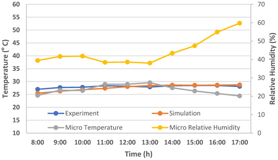
Figure 6.
Comparison between measurements and simulation outcomes from EnergyPlus.
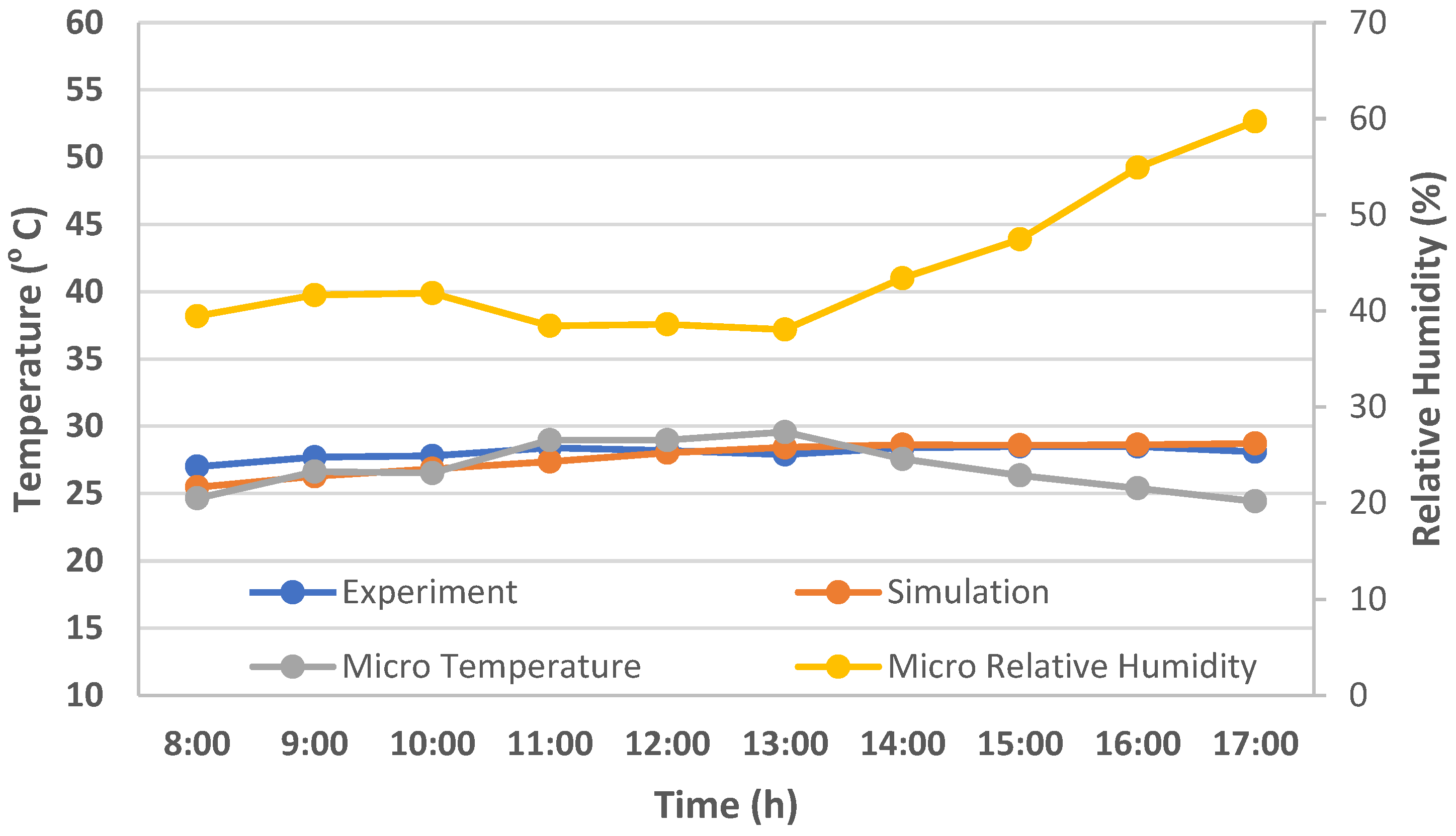
3.1.2. Results of ENVI-met Model Validation
The outcomes of ENVI-met were validated by comparisons with the measurement results in Section 3.1.1. The hourly room temperature and relative humidity in four directions around the target building were averaged and compared with the average microclimate data around the target building. The simulation results are shown in Figure 7. It can be observed that the temperature differences between experimental and simulation outcomes were in the range of −1.00–1.03 °C (−4.46–3.54%), indicating good agreement.
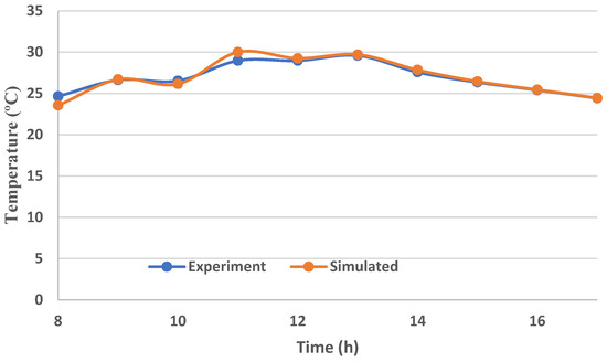
Figure 7.
Comparison between measurements and simulation outcomes from ENVI-met.
3.1.3. Results of k-Fold Cross-Validation on BPNN Model
K-fold cross-validation has been conducted to verify the robustness of the BPNN model. Table 6 lists the results from k-fold cross-validation. It can be found that for each fold of test set samples, the R-squares are higher than 0.945 for the IDDHs model and higher than 0.968 for the BEC model, which ensures the model robustness and prediction accuracy.
Table 6.
Results of k-fold cross-validation of BPNN model.
3.2. Results of ENVI-Met and EnergyPlus
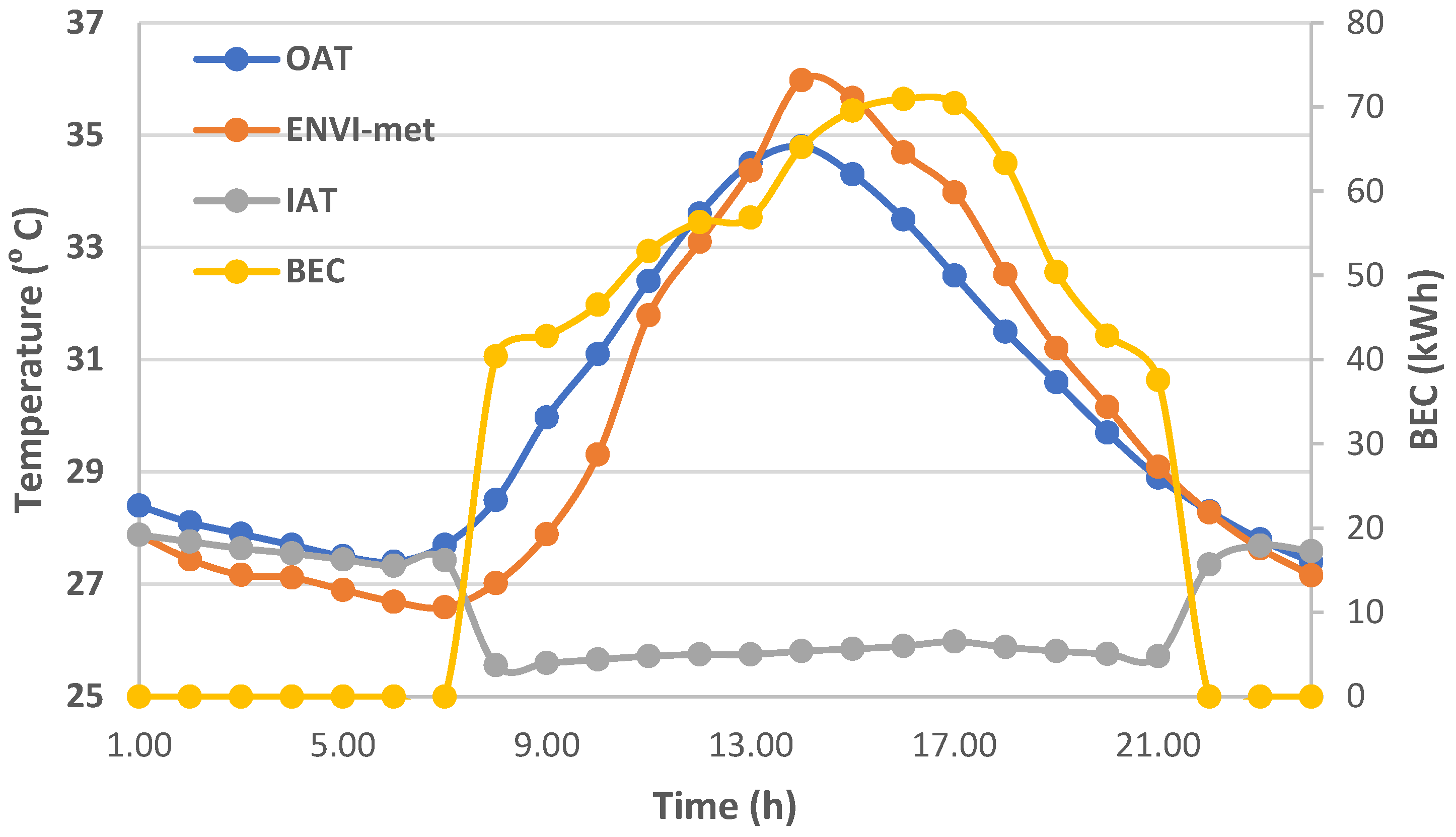
The simulation results from ENVI-met and EnergyPlus on January 21 and July 21 for the base case building are presented in Figure 8 and Figure 9, respectively. It can be observed that in winter, the average micro-climate temperatures from ENVI-met were consistently lower (1.4–2.0 °C) than the outdoor air temperature, while in summer, the average micro-climate temperatures from ENVI-met were slightly lower (0.1–2.0 °C) than the outdoor air temperature while being slightly higher in the afternoon and then close to the outdoor air temperature. In winter, the energy consumption was more or less flat while in summer the energy consumption had a similar trend to the micro-climate and outdoor air temperature with a time delay of 3 h.
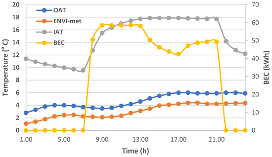
Figure 8.
Outcomes from ENVI-met and EnergyPlus for the base case on 21 January.
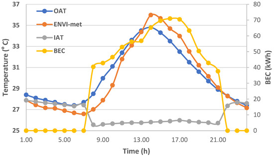
Figure 9.
Outcomes from ENVI-met and EnergyPlus for the base case on 21 July.
3.3. Prediction Model Performance Comparision
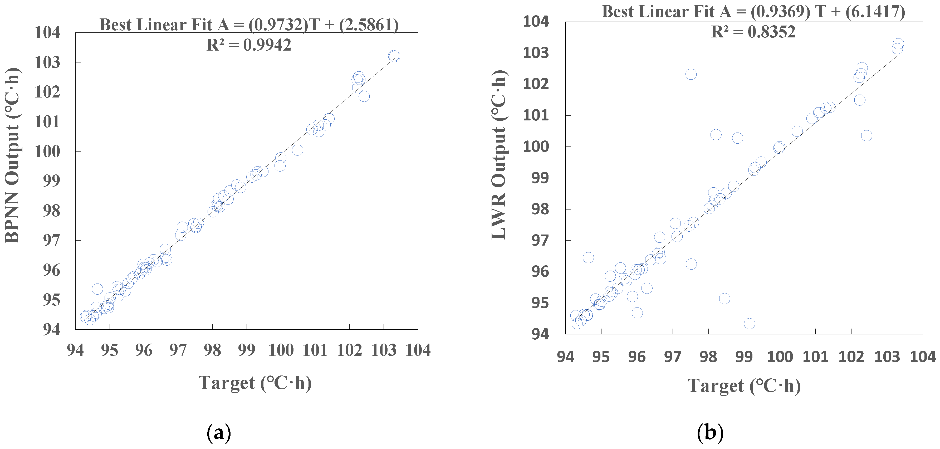
Figure 10a,b present the regressions between prediction and simulation results of IDDHs for the two ML models.
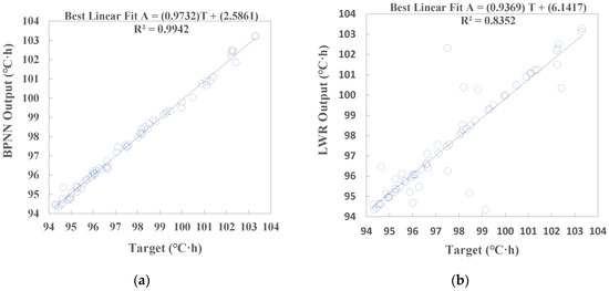
Figure 10.
Regression between prediction and simulation results of IDDHs. (a) BPNN model; (b) LWR model.
The R-squares are 0.9942 and 0.8352, respectively. The BPNN model obviously outperforms the LWR model. The accuracies of the BPNN model are comparable with the outcomes from [23,24,25], where the R-squares are in the range of 0.96–0.998.
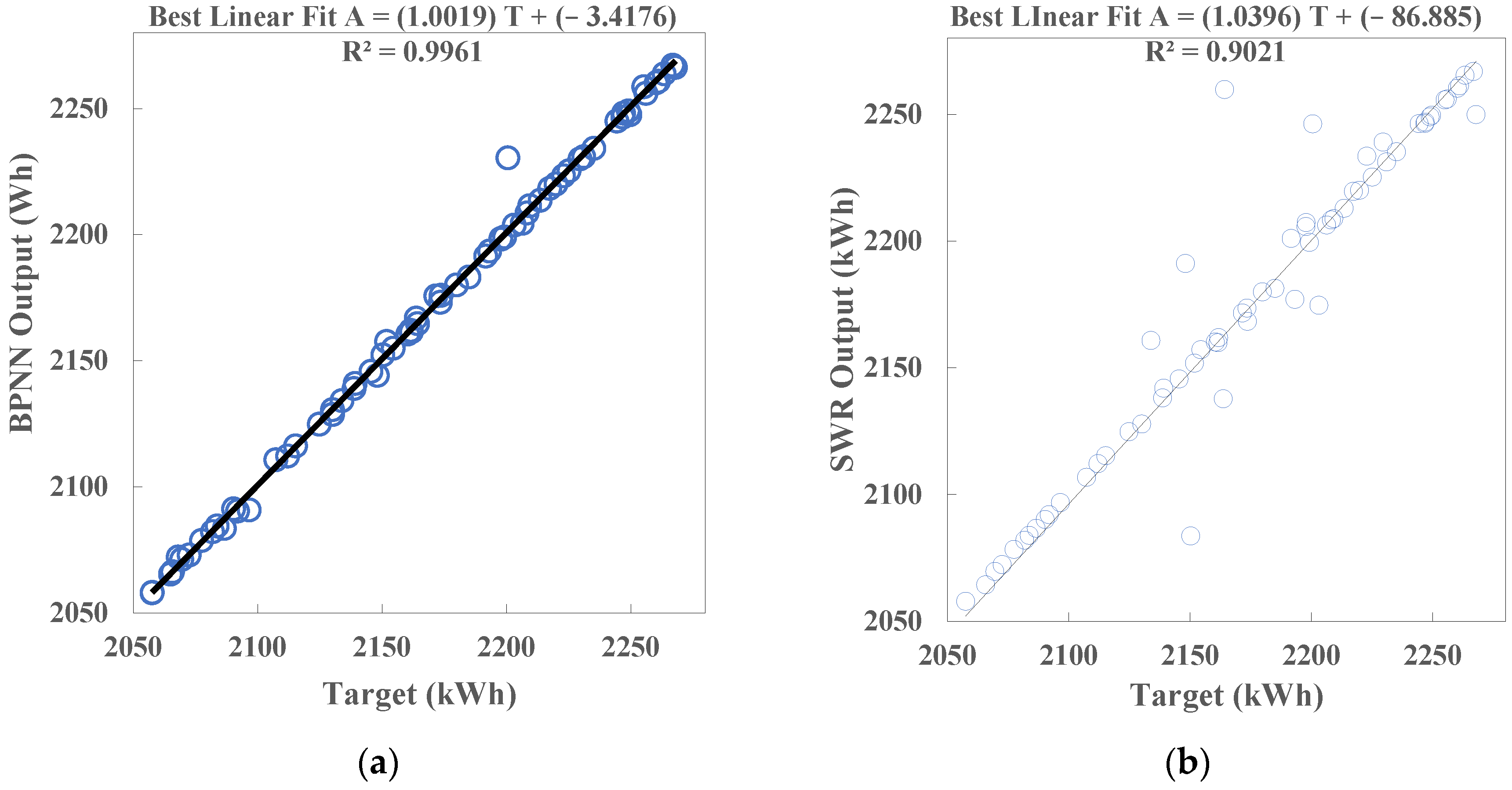
Figure 11a,b present the regressions between prediction and simulation results of BEC for the two ML models.
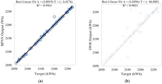
Figure 11.
Regression between prediction and simulation results of BEC. (a) BPNN model; (b) LWR model.
The R-squares are 0.9961 and 0.9021, respectively. Similarly, the BPNN model outperforms the LWR model. The accuracies of the BPNN model are comparable with the outcomes from [23,24,26], where the R-squares are between 0.990 and 0.997.
Table 7 presents the error distribution for the two prediction models. It can be observed that the BPNN models outperforms the LWR models, with maximum absolute relative errors of less than 1% for predicting IDDHs (in the range of 0.56~0.76%) and less than 2% for predicting BEC (in the range of −0.28~1.36%). Therefore, the BPNN models should be selected for further analysis. The maximum errors are less than the ones in Ref. [35] with 6.01% for building thermal load prediction and 3.51% for IDDHs prediction, which means that the BPNN models using the outdoor physical parameters are feasible and can be used for optimization purposes.
Table 7.
Relative absolute errors distribution for IDDHs and BEC.
3.4. Optimization Algorithm Performance Comparision
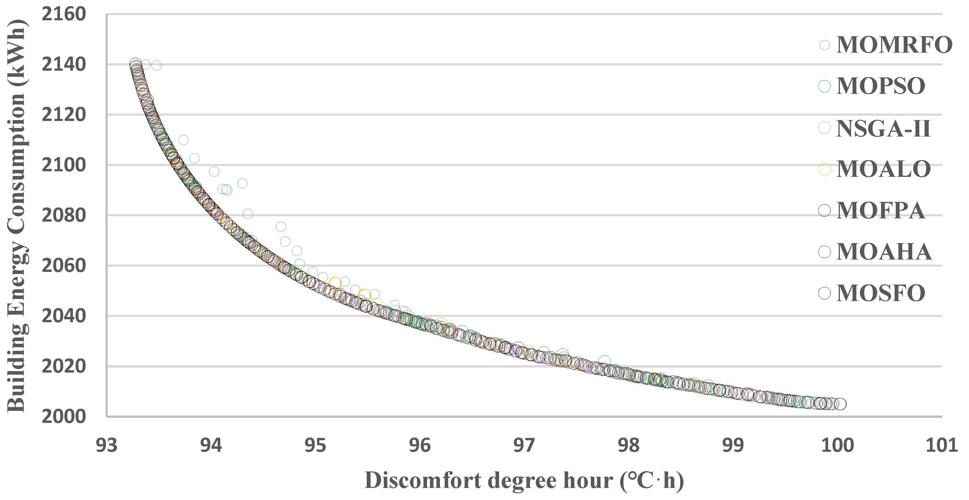
The BPNN prediction models served as fitness functions for seven optimization algorithms, including MOPSO, NSGA-II, MOALO, MOAHA, MOFPA, MOSFO, and MOMRFO to find Pareto solutions. The process is repeated as many times as possible to find all the potential optimal solutions.
Figure 12 compares the Pareto solutions obtained by all the optimization algorithms. Overall, all the Pareto fronts share similar trends. The ones obtained by the MOPSO, MOALO, and MOMRFO algorithms have obvious segments, while those obtained by the NASA-II, MOAHA, MOFPA, and MOSFO algorithms have coherent Pareto fronts. The MOAHA algorithm has slightly better performance than the others as it provides more solutions with coherent Pareto fronts. The discomfort degree hours are in the range of 93~100 °C∙h, while the building energy consumption is in the range of 2000~2140 kWh. The IDDHs decrease with the increase in BEC. A maximum reduction of 1.3 °C in OAT in summer was observed during the analysis.
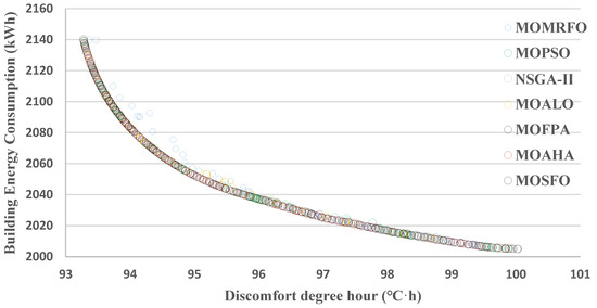
Figure 12.
Pareto solution sets.
Table 8 compares the performance of each optimization algorithm. It can be observed that the number of generations reaches 151–185 when converged, and the computation time takes about 109 to 155 s. MOAHA outperforms other algorithms in terms of number of iterations and computation time.
Table 8.
Comparison of optimization algorithm performance.
3.5. Optimal Solutions Analysis
To compare the performance of each optimization algorithm, six indicators, , , , , , and , were introduced and calculated via Equations (8)–(13):
where Umax and are the maximum and average reduction rates in IDDHs, respectively; and are the maximum and average reduction rates in BEC, respectively; and are the maximum and average reduction rates in air-conditioning system energy consumption, respectively; Tr is the IDDHs of the reference building, in °C·h; Tmin is the minimum IDDHs among the optimal solutions, in °C·h; Ti is the IDDHs of the ith solution, in °C·h; Er is the BEC of the reference building, in kWh; Emin is the minimum BEC among the optimal solutions, in °C·h; Ei is the BEC of the ith solution, in kWh; n is the number of optimal solutions; is the air-conditioning system energy consumption (ACSEC) of the reference building, in kWh; is the minimum ACSEC among the optimal solutions, in kWh; El and Ee are the lighting and electrical equipment energy consumption, in kWh; is the ACSEC of the ith solution, in kWh.
Table 9 summarizes the values of the performance evaluation indicators for all the optimization algorithms. It can be found that the maximum reduction rates in IDDHs from the outcomes of the MOPSO, NSGA-II, MOAHA, MOFPA, and MOSFO optimization algorithms are 7.45%. The reduction rates from the outcomes of the MOALO and MOMRFO optimization algorithms are slightly lower, which are 7.39% and 7.36%, respectively. The average reduction rates of the outcomes of all the optimization algorithms range from 4.9~6%, with MOALO having the highest at 6% and MOMRFO the lowest at 3.69%. The maximum reduction rates in BEC from the outcomes of all the optimization algorithms range from 3.81~4.13%. MOFPA and MOSFO achieve the highest reduction rate and MOALO achieves the lowest. The average reduction rates from the outcomes of all the optimization algorithms range from 0.9~2.75%, with MOMRFO having the lowest reduction rate and MOMRFO having the highest. Previous studies also showed that a change in pavement material reflectivity can lead to a 0.2–2.5% reduction in BEC in Cairo [15], surrounding building shading can help reduce the BEC by 2.69% [5], an increase of 17% in the tree coverage rate could lower the maximum temperature by 1.1 °C on the hottest summer day [8], and greening can reduce the IAT by 0.6–1.5 °C [7]. The multi-objective optimization led to a maximum energy reduction of 4.12% (86.16 kWh, or CNY 53 (with an electricity price of CNY 0.617/kWh), or 51.19 kgCO2-eq (0.5942 kgCO2/kWh)), a 7.45% (7.4 °C·h) improvement in thermal comfort, and a 1.3 °C reduction in OAT in summer.
Table 9.
Performance evaluation of different optimization algorithms.
As shown in Figure 7 and Table 5, MOAHA can find most of the optimal solutions and achieve satisfactory optimization results, and therefore the outcomes from the MOAHA algorithm were selected for further analysis.
Table 10 lists 20 representative optimal solutions based on the MOAHA algorithm. The optimal solutions were found to prefer a low pavement albedo of 0.04~0.054, a greening rate around 0.15, and offsets of surrounding buildings from the original position by approximately 0~1.4 m.
Table 10.
20 representative optimal solutions.
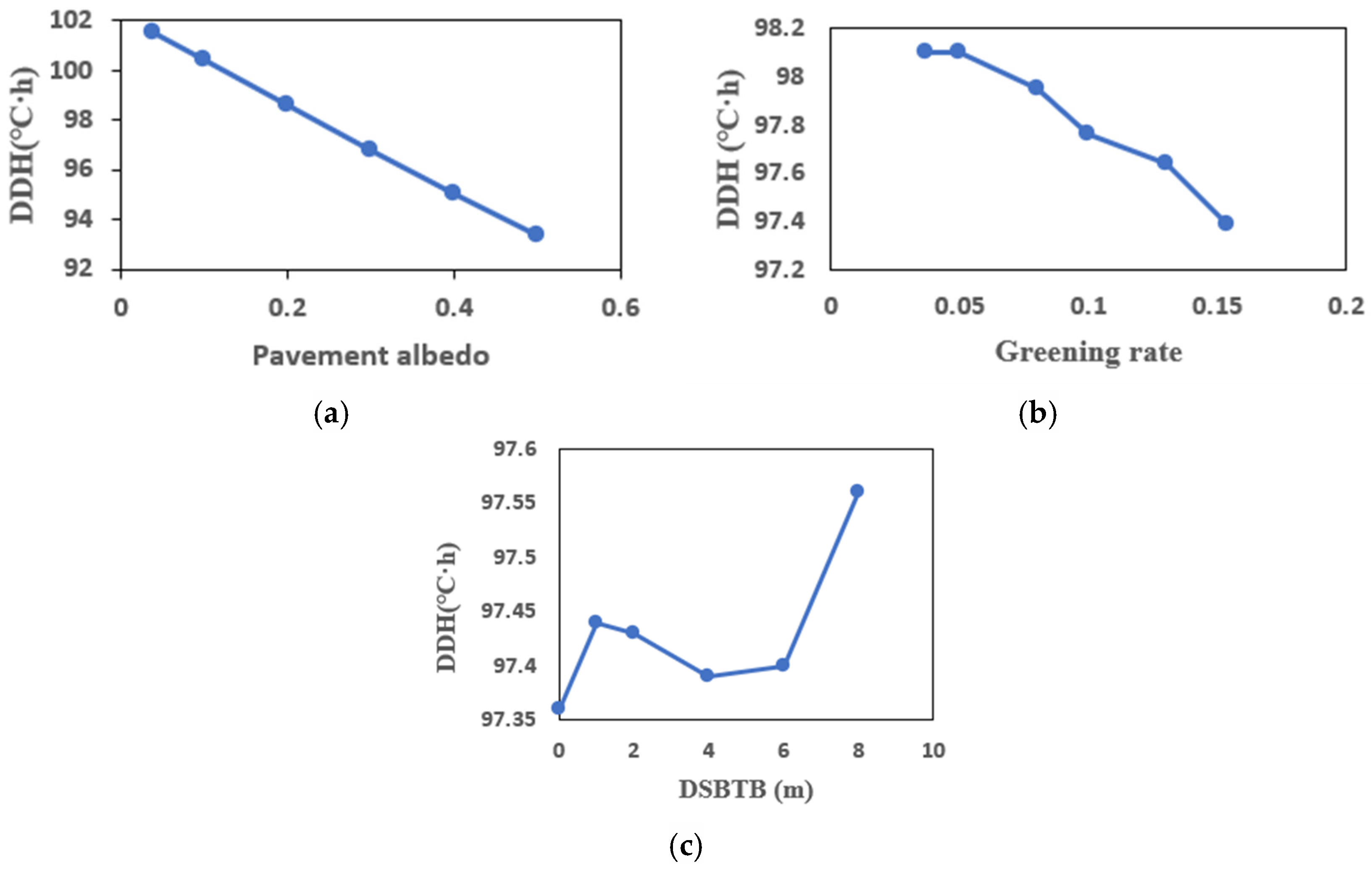
Figure 13 presents the sensitivity analysis of the impact of each design parameter on IDDHs. It can be observed that the IDDHs decrease with the increase in pavement albedo and greening rate. As for the DSBTB, IDDHs increase with DSBTB before it increases to 1 m and then decrease till it reaches 4 m and then increase again.

Figure 13.
Sensitivity analysis of the impact of design parameters on IDDHs. (a) Pavement albedo; (b) greening rate; (c) DSBTB.
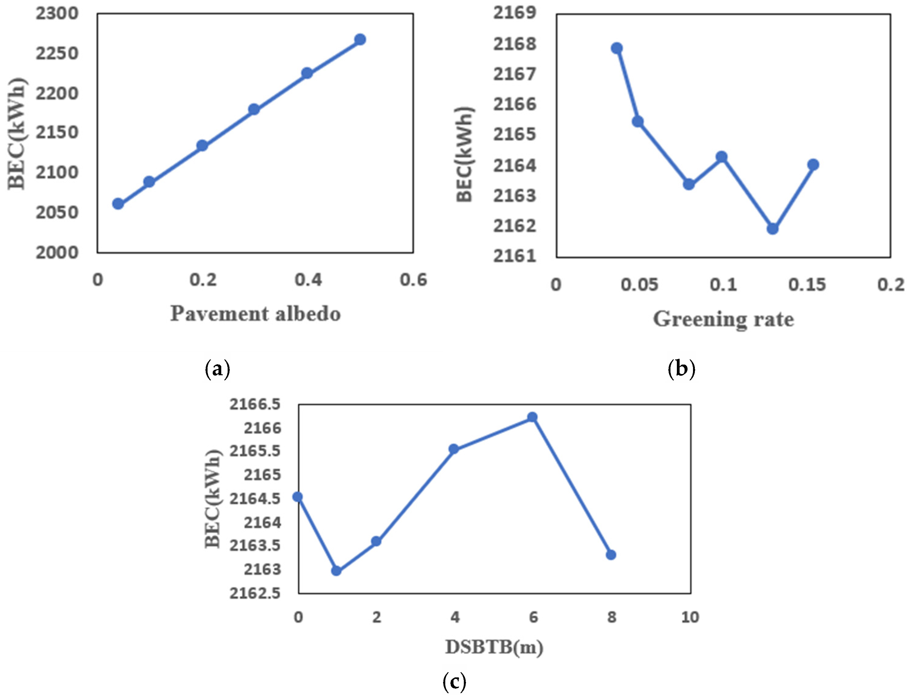
Figure 14 presents the sensitivity analysis on the impact of each design parameter on BEC. It can be observed that BEC increases with the increase in pavement albedo. It decreases with the greening rate before it reaches 0.13 and then slightly increases again. As for the DSBTB, BEC decreases with DSBTB before it increases to 1 m and then decreases till it reaches 6 m and then decreases again.

Figure 14.
Sensitivity analysis of the impact of design parameters on BEC. (a) Pavement albedo; (b) greening rate; (c) DSBTB.
As the study focuses on a campus building in the HSCW climate region in Shanghai, the outcomes of the study cannot be directly applied to other types of buildings in other climate regions. However, the research framework can be adapted to other building types in other climate regions, and even expanded to the optimization of different building design parameters. For example, during the design sample generation process, building design parameters, such as building orientation, insulation level, window-to-wall ratio, etc., can be selected and generated together with the outdoor physical parameters to perform co-optimization of outdoor and building design parameters.
4. Conclusions
A comprehensive method was developed to optimize the physical design parameters of the outdoor environment to reduce the indoor discomfort degree hours and energy consumption for an office building in Shanghai, China. A four-step research framework was applied to perform design optimization. The surrounding building distance, pavement albedo, and greening rate were selected as the design parameters and sampled using the Latin hypercube sampling approach. BPNN and LWR prediction models were developed as potential fitness functions for seven optimization algorithms. It can be concluded that:
- (1)
- The R-squares of the BPNN models for predicting IDDHs and BEC are 0.9942 and 0.996, respectively, with maximum absolute relative errors less than 2%, indicating the BPNN models outperform the LWR models;
- (2)
- It can be found from the outcomes of the Pareto solutions of all the optimization algorithms that the reduction rate in IDDHs is greater than that in BEC;
- (3)
- The MOAHA algorithm outperforms other optimization algorithms in terms of solution quality, speed (109 s), and convergence (reaching convergence at 151 generations) and achieves maximum reductions in IDDHs and BEC of 7.45% and 4.12%, respectively. The average reduction in IDDHs and BEC is 4.99% and 1.70%, respectively;
- (4)
- The Pareto solutions indicate that for a climate with hot summers and cold winters, setting the road surface albedo to the lowest value and the greening rate to the highest value can achieve the best indoor thermal environment.
This study contributes to the development of the optimal multi-objective design of the outdoor physical parameters of an office building. Its originality includes the application of a four-step research framework, evaluation of the prediction models’ and optimization algorithm’s performance, as well as the impact of multiple outdoor physical parameters. It can practically guide the urban planner in performing outdoor design to reduce indoor discomfort and improve building energy performance.
Future studies involve more outdoor physical parameters, e.g., sky view factor, water bodies, as well as co-optimization of outdoor physical parameters and building envelope design parameters, more climatic regions, and practical engineering applications.
Author Contributions
Conceptualization, Y.L. and W.Y.; methodology, Y.L. and W.Y.; formal analysis, Y.L.; investigation, T.H.; resources, Y.L.; writing—original draft preparation, T.H.; writing—review and editing, Y.L., T.H., W.Y., M.C. and C.-Q.L.; supervision, Y.L.; funding acquisition, Y.L.; validation, M.D. and P.C. All authors have read and agreed to the published version of the manuscript.
Funding
This work is financially supported by the National Natural Science Foundation of China, grant number 52268002.
Data Availability Statement
The original contributions presented in this study are included in the article. Further inquiries can be directed to the corresponding authors.
Acknowledgments
The authors express their sincere gratitude to the support from the R & D center of the transportation industry of health and epidemic prevention technology, Ministry of Transportation of the People’s Republic of China.
Conflicts of Interest
The authors declare no conflicts of interest.
Abbreviations
The following abbreviations and symbols are used in this manuscript:
| ACSEC | Air-conditioning system energy consumption |
| AHOA | Artificial hummingbird optimization algorithm |
| ALO | Antlion Optimizer |
| ANN | Artificial Neural Network |
| BEC | Building energy consumption |
| BPNN | Backpropagation neural network |
| CDDH | Cooling discomfort degree hour |
| DSBTB | Distance between surrounding buildings and targeted building |
| H/W | Height to street wide (H/W) |
| HDDH | Heating discomfort degree hour |
| HSCW | Hot summer and cold winter |
| IAT | Indoor air temperature |
| IDDHs | Indoor discomfort degree hours |
| LHS | Latin Hypercube Sampling |
| LWR | Locally weighted regression |
| ML | Machine learning |
| MLR | Multiple Linear Regression |
| MOAHA | Multi-Objective Artificial Hummingbird Algorithm |
| MOFPA | Multi-objective Flower Pollination Algorithm |
| MOMRFO | Multi-objective Manta Ray Foraging Optimizer |
| MOPSO | Multi-Objective Particle Swarm Optimization |
| MOSFO | Multi-objective Sunflower Optimization |
| NSGA-II | Nondominated Sorting Genetic Algorithm version II |
| PSO | Particle Swarm Optimization |
| SVR | Support Vector Regression |
| f1 | IDDHs, °C∙h |
| f2 | BEC, kWh |
| IC | CDDHs, °C∙h |
| IH | HDDHs, °C∙h |
| IAT at time i, °C | |
| tH | The higher thermal comfort temperature limits, taken as 26 °C |
| tL | The lower thermal comfort temperature limits, taken as 18 °C |
| m | the numbers of nodes of input layer |
| a | the numbers of nodes of input variables |
| b | the numbers of nodes of output variables |
| c | a constant, 0~10 |
| W | the Gaussian kernel function |
| k | the rate at which the weight changes with distance |
| X | the independent variable |
| Y | the dependent variable |
| Umax | the maximum reduction rates in IDDHs |
| the average reduction rates in IDDHs | |
| the maximum reduction rates on BEC | |
| the average reduction rates on BEC | |
| the maximum reduction rates in air-conditioning system energy consumption | |
| the average reduction rates in air-conditioning system energy consumption | |
| Tr | the IDDHs of the reference building, °C·h |
| Tmin | the minimum IDDHs among the optimal solutions, °C·h |
| Ti | the IDDHs of the ith solution, °C·h |
| Er | the BEC of the reference building, kWh |
| Emin | the minimum BEC among the optimal solutions, °C·h |
| n | the number of optimal solutions |
| the ACSEC of the reference building, kWh | |
| the minimum ACSEC among the optimal solutions, kWh | |
| El | the lighting energy consumption, kWh |
| Ee | the electrical equipment energy consumption, kWh |
| the ACSEC of the ith solution, kWh |
References
- Lin, Y.; Huang, T.; Yang, W.; Hu, X.; Li, C. A Review on the Impact of Outdoor Environment on Indoor Thermal Environment. Buildings 2023, 13, 2600. [Google Scholar] [CrossRef]
- Liu, H.; Pan, Y.; Yang, Y.; Huang, Z. Evaluating the impact of shading from surrounding buildings on heating/ cooling energy demands of different community forms. Build. Environ. 2021, 206, 108322. [Google Scholar] [CrossRef]
- Strømann-Andersen, J.; Sattrup, P.A. The urban canyon and building energy use: Urban density versus daylight and passive solar gains. Energy Build. 2011, 43, 2011–2020. [Google Scholar] [CrossRef]
- Yaghoobian, N.; Kleissl, J. Effect of reflective pavements on building energy use. Urban. Clim. 2012, 2, 25–42. [Google Scholar] [CrossRef]
- Ichinose, T.; Lei, L.; Lin, Y. Impacts of shading effect from nearby buildings on heating and cooling energy consumption in hot summer and cold winter zone of China. Energy Build. 2017, 136, 199–210. [Google Scholar] [CrossRef]
- Deng, Q.; Wang, G.; Wang, Y.; Zhou, H.; Ma, L. A quantitative analysis of the impact of residential cluster layout on building heating energy consumption in cold IIB regions of China. Energy Build. 2021, 253, 111515. [Google Scholar] [CrossRef]
- Morakinyo, T.E.; Dahanayake, K.W.D.K.C.; Adegun, O.B.; Balogun, A.A. Modelling the effect of tree-shading on summer indoor and outdoor thermal condition of two similar buildings in a Nigerian university. Energy Build. 2016, 130, 721–732. [Google Scholar] [CrossRef]
- Taleghani, M.; Marshall, A.; Fitton, R.; Swan, W. Renaturing a microclimate: The impact of greening a neighbourhood on indoor thermal comfort during a heatwave in Manchester, UK. Sol. Energy 2019, 182, 245–255. [Google Scholar] [CrossRef]
- Simpson, J.R.; McPherson, E.G. Simulation of tree shade impacts on residential energy use for space conditioning in Sacramento. Atmos. Environ. 1998, 32, 69–74. [Google Scholar] [CrossRef]
- Darvish, A.; Eghbali, G.; Eghbali, S.R. Tree-configuration and species effects on the indoor and outdoor thermal condition and energy performance of courtyard buildings. Urban. Clim. 2021, 37, 100861. [Google Scholar] [CrossRef]
- Akbari, H.; Kurn, D.M.; Bretz, S.E.; Hanford, J.W. Peak power and cooling energy savings of shade trees. Energy Build. 1997, 25, 139–148. [Google Scholar] [CrossRef]
- Li, Z.; Chow, D.H.C.; Yao, J.; Zheng, X.; Zhao, W. The effectiveness of adding horizontal greening and vertical greening to courtyard areas of existing buildings in the hot summer cold winter region of China: A case study for Ningbo. Energy Build. 2019, 196, 227–239. [Google Scholar] [CrossRef]
- Synnefa, A.; Karlessi, T.; Gaitani, N.; Santamouris, M.; Assimakopoulos, D.N.; Papakatsikas, C. Experimental testing of cool colored thin layer asphalt and estimation of its potential to improve the urban microclimate. Build. Environ. 2011, 46, 38–44. [Google Scholar] [CrossRef]
- Carnielo, E.; Zinzi, M. Optical and thermal characterisation of cool asphalts to mitigate urban temperatures and building cooling demand. Build. Environ. 2013, 60, 56–65. [Google Scholar] [CrossRef]
- Aboelata, A. Reducing outdoor air temperature, improving thermal comfort, and saving buildings’ cooling energy demand in arid cities—Cool paving utilization. Sustain. Cities Soc. 2021, 68, 102762. [Google Scholar] [CrossRef]
- Salvati, A.; Kolokotroni, M.; Kotopouleas, A.; Watkins, R.; Giridharan, R.; Nikolopoulou, M. Impact of reflective materials on urban canyon albedo, outdoor and indoor microclimates. Build. Environ. 2022, 207, 108459. [Google Scholar] [CrossRef]
- Jandaghian, Z.; Berardi, U. Analysis of the cooling effects of higher albedo surfaces during heat waves coupling the Weather Research and Forecasting model with building energy models. Energy Build. 2020, 207, 109627. [Google Scholar] [CrossRef]
- Santamouris, M.; Haddad, S.; Saliari, M.; Vasilakopoulou, K.; Synnefa, A.; Paolini, R.; Ulpiani, G.; Garshasbi, S.; Fiorito, F. On the energy impact of urban heat island in Sydney: Climate and energy potential of mitigation technologies. Energy Build. 2018, 166, 154–164. [Google Scholar] [CrossRef]
- Xu, X.; AzariJafari, H.; Gregory, J.; Norford, L.; Kirchain, R. An integrated model for quantifying the impacts of pavement albedo and urban morphology on building energy demand. Energy Build. 2020, 211, 109759. [Google Scholar] [CrossRef]
- Kleissl, J.; Yaghoobian, N.; Krayenhoff, E.S. Modeling the Thermal Effects of Artificial Turf on the Urban Environment. J. Appl. Meteorol. Climatol. 2010, 49, 332–345. [Google Scholar]
- Qin, Y. Urban canyon albedo and its implication on the use of reflective cool pavements. Energy Build. 2015, 96, 86–94. [Google Scholar] [CrossRef]
- Li, H.; Harvey, J.; Kendall, A. Field measurement of albedo for different land cover materials and effects on thermal performance. Build. Environ. 2013, 59, 536–546. [Google Scholar] [CrossRef]
- Wang, W.; Zhang, L. Influence of subway entrance layout on indoor and outdoor environments in street canyons with different geometric form. J. Clean. Prod. 2023, 425, 138784. [Google Scholar] [CrossRef]
- Du, L.; Wang, H.; Bian, C.; Chen, X. Impact of block form on building energy consumption, urban microclimate and solar potential: A case study of Wuhan, China. Energy Build. 2025, 328, 115224. [Google Scholar] [CrossRef]
- Gonçalves, E.L.S.; Braga, J.L.; de Oliveira Sampaio, A.; dos Santos Batista, V.; da Rocha Menezes, L.J.; Eli, L.G.; Barata, M.S.; da Silva Ventura Neto, R.; Zemero, B.R. Multiscale modeling to optimize thermal performance design for urban social housing: A case study. Appl. Therm. Eng. 2024, 236, 121379. [Google Scholar] [CrossRef]
- Wu, C.; Pan, H.; Luo, Z.; Liu, C.; Huang, H. Multi-objective optimization of residential building energy consumption, daylighting, and thermal comfort based on BO-XGBoost-NSGA-II. Build. Environ. 2024, 254, 111386. [Google Scholar] [CrossRef]
- Chen, Z.; Cui, Y.; Zheng, H.; Ning, Q.; Wang, Y.; Hu, L.; Hou, L.; Cai, W.; Wang, L.; He, Y. Study on energy consumption, thermal comfort and economy of passive buildings based on multi-objective optimization algorithm for existing passive buildings. J. Clean. Prod. 2023, 425, 138760. [Google Scholar]
- Ismail, N.; Ouahrani, D. A comprehensive optimization study of personal cooling radiant desks integrated to HVAC system for energy efficiency and thermal comfort in office buildings. Int. J. Refrig. 2023, 156, 54–71. [Google Scholar] [CrossRef]
- Hosamo, H.H.; Tingstveit, M.S.; Nielsen, H.K.; Svennevig, P.R.; Svidt, K. Multiobjective optimization of building energy consumption and thermal comfort based on integrated BIM framework with machine learning-NSGA II. Energy Build. 2022, 277, 112479. [Google Scholar] [CrossRef]
- Zhang, Y.; Lin, K.; Zhang, Q.; Di, H. Ideal thermophysical properties for free-cooling (or heating) buildings with constant thermal physical property material. Energy Build. 2006, 38, 1164–1170. [Google Scholar] [CrossRef]
- JGJ 134-2010; Design Standard for Energy Efficiency of Residential Buildings in Hot Summer and Cold Winter Zone. China Construction Industry Press: Beijing, China, 2010.
- GB55015-2021; General Code for Energy Efficiency and Renewable Energyapplication in Buildings. China Construction Industry Press: Beijing, China, 2021.
- Yang, X.; Zhao, L.; Bruse, M.; Meng, Q. An integrated simulation method for building energy performance assessment in urban environments. Energy Build. 2012, 54, 243–251. [Google Scholar] [CrossRef]
- McKay, M.D.; Beckman, R.J.; Conover, W.J. A Comparison of Three Methods for Selecting Values of Input Variables in the Analysis of Output From a Computer Code. Technometrics 2000, 42, 55–61. [Google Scholar] [CrossRef]
- Lin, Y.; Zhou, S.; Yang, W.; Li, C.-Q. Design Optimization Considering Variable Thermal Mass, Insulation, Absorptance of Solar Radiation, and Glazing Ratio Using a Prediction Model and Genetic Algorithm. Sustainability 2018, 10, 336. [Google Scholar] [CrossRef]
- Mihalakakou, G.; Santamouris, M.; Tsangrassoulis, A. On the energy consumption in residential buildings. Energy Build. 2002, 34, 727–736. [Google Scholar] [CrossRef]
- Ruano, A.E.; Crispim, E.M.; Conceição, E.Z.E.; Lúcio, M.M.J.R. Prediction of building’s temperature using neural networks models. Energy Build. 2006, 38, 682–694. [Google Scholar] [CrossRef]
- Mirzaei, P.A.; Olsthoorn, D.; Torjan, M.; Haghighat, F. Urban neighborhood characteristics influence on a building indoor environment. Sustain. Cities Soc. 2015, 19, 403–413. [Google Scholar] [CrossRef]
- Rumelhart, D.E.; Hinton, G.E.; Williams, R.J. Learning representations by back-propagating errors. Nature 1986, 323, 533–536. [Google Scholar] [CrossRef]
- Cleveland, W.S.; Devlin, S.J. Locally Weighted Regression: An Approach to Regression Analysis by Local Fitting. J. Am. Stat. Assoc. 1988, 83, 596–610. [Google Scholar] [CrossRef]
- Kennedy, J.; Eberhart, R. Particle swarm optimization. In Proceedings of the ICNN’95-International Conference on Neural Networks, Perth, WA, Australia, 27 November–1 December 1995. [Google Scholar]
- Coello, C.A.C.; Lechuga, M.S. MOPSO: A proposal for multiple objective particle swarm optimization. In Proceedings of the 2002 Congress on Evolutionary Computation CEC’02 (Cat No. 02TH8600), Honolulu, HI, USA, 12–17 May 2002. [Google Scholar]
- Deb, K.; Pratap, A.; Agarwal, S.; Meyarivan, T. A fast and elitist multiobjective genetic algorithm: NSGA-II. IEEE Trans. Evol. Comput. 2002, 6, 182–197. [Google Scholar] [CrossRef]
- Mirjalili, S.; Jangir, P.; Saremi, S. Multi-objective ant lion optimizer: A multi-objective optimization algorithm for solving engineering problems. Appl. Intell. 2016, 46, 79–95. [Google Scholar] [CrossRef]
- Mirjalili, S. The Ant Lion Optimizer. Adv. Eng. Software 2015, 83, 80–98. [Google Scholar] [CrossRef]
- Khodadadi, N.; Mirjalili, S.M.; Zhao, W.; Zhang, Z.; Wang, L.; Mirjalili, S. Multi-Objective Artificial Hummingbird Algorithm. In Advances in Swarm Intelligence; Kacprzyk, J., Ed.; Springer: Gewerbestrasse, Switzerland, 2023; Volume 1054, pp. 407–419. [Google Scholar]
- Yang, X.-S.; Karamanoglu, M.; He, X. Flower pollination algorithm: A novel approach for multiobjective optimization. Eng. Optim. 2013, 46, 1222–1237. [Google Scholar] [CrossRef]
- Yang, X.-S. Flower pollination algorithm for global optimization. In Proceedings of the International Conference on Unconventional Computing and Natural Computation, Orléan, France, 3–7 September 2012. [Google Scholar]
- Pereira, J.L.J.; Gomes, G.F. Multi-objective sunflower optimization: A new hypercubic meta-heuristic for constrained engineering problems. Expert Syst. 2023, 40, 13331. [Google Scholar] [CrossRef]
- Got, A.; Zouache, D.; Moussaoui, A. MOMRFO: Multi-objective Manta ray foraging optimizer for handling engineering design problems. Knowl.-Based Syst. 2022, 237, 107880. [Google Scholar] [CrossRef]
- Zhao, W.; Zhang, Z.; Wang, L. Manta ray foraging optimization: An effective bio-inspired optimizer for engineering applications. Eng. Appl. Artif. Intell. 2020, 87, 103300. [Google Scholar] [CrossRef]
- Lin, Y.; Wang, J.; Yang, W.; Chan, M.; Hu, X. A Case Study of Multi-objective Design Optimization of a Healthy Building in Shanghai, China. J. Build. Eng. 2024, 96, 110581. [Google Scholar] [CrossRef]


Disclaimer/Publisher’s Note: The statements, opinions and data contained in all publications are solely those of the individual author(s) and contributor(s) and not of MDPI and/or the editor(s). MDPI and/or the editor(s) disclaim responsibility for any injury to people or property resulting from any ideas, methods, instructions or products referred to in the content. |
© 2025 by the authors. Licensee MDPI, Basel, Switzerland. This article is an open access article distributed under the terms and conditions of the Creative Commons Attribution (CC BY) license (https://creativecommons.org/licenses/by/4.0/).