Research on Fracture Energy Prediction and Size Effect of Concrete Based on Deep Learning with SHAP Interpretability Method

Abstract

Fracture energy plays a pivotal role in ensuring the safe design of concrete structures. Currently, experimental testing remains the predominant methodology for exploring fracture energy in concrete. Nevertheless, this approach is hindered by protracted sample production cycles and test loading conditions that contribute to elevated expenses. Moreover, owing to the complex nonlinear behavior exhibited by concrete during the fracturing process, existing empirical formulas exhibit restricted precision when forecasting fracture energy. Therefore, in order to swiftly and accurately predict the fracture energy of concrete and investigate the impact of various factors on it, this study employs a deep learning algorithm to establish the correlation between parameters and fracture energy. Additionally, an interpretable deep learning prediction model for fracture energy is proposed, which is then compared with existing empirical formulas. Finally, the SHapley Additive exPlanations (SHAP) interpretability method is utilized to interpret and analyze the prediction results. The SHAP method can identify and visualize the contribution direction (positive/negative) and magnitude of the input features and reveal the relative importance of parameters at both local and global levels simultaneously. This analysis effectively explains the decision-making mechanism of the “black box” model and significantly improves the problem of insufficient interpretability that is common in traditional machine learning methods. The findings demonstrate that over 87% of the prediction results from the deep learning model in this study exhibit a relative error of less than 10% on the test set. The model effectively captures the intricate nonlinear relationship among characteristic parameters, exhibiting superior accuracy and generalization capabilities compared to empirical formulas. The SHAP values of the input parameters are visualized to assess their influence on fracture energy: initially, fracture energy increases and then decreases with increasing compressive strength, age, and coarse aggregate proportion; fracture energy increases with increasing maximum particle size of aggregate until it reaches 20 mm, after which it stabilizes; a high water–binder ratio reduces fracture energy; within the range of 400 mm, fracture energy increases with height, exhibiting a noticeable size effect; fracture energy increases with specimen width, but the size effect diminishes beyond 150 mm width; fracture energy decreases as span–height ratio increases; seam height ratio exhibits an initial increase followed by a decrease in fracture energy, with larger ratios showing a more pronounced size effect; an increase in ligament height enhances fracture energy while maintaining a significant size effect.

1. Introduction

The corrosion resistance and higher compressive strength of concrete make it a widely used material for building structure-bearing components. However, concrete structures are prone to crack and then fracture when bearing tensile loads, which reduces the safety and durability of building structures. In the field of nonlinear fracture theory of concrete, which has been gradually developed since the 1970s, fracture energy has become a key concept for describing the fracture performance of concrete. Fracture energy refers to the amount of energy required to characterize crack propagation per unit area and holds important academic significance as well as practical application value. Accurate application of concrete nonlinear fracture theory requires prior knowledge of parameters such as fracture energy. Accurate prediction of concrete fracture energy is critically important for structural safety design [1]. A reliable tool for the rapid estimation of fracture energy can help reduce both the conservatism and potential risks arising from deviations in empirical formulas, thereby enhancing the rationality, cost-effectiveness, and safety of concrete structural analysis and design. This concept has been validated by numerous experimental and analytical studies [2,3].

The fracture energy of concrete is typically determined by testing it according to a series of test standards [4,5]. The direct tensile method [6] is theoretically the most accurate approach for measuring concrete fracture energy; however, it demands advanced equipment and has a low success rate. As a result, the currently employed methods include the three-point bending beam method [7,8] and the wedge splitting method [9,10]. The three-point bending method has been adopted by RILEM as the recommended method for testing the fracture energy of concrete [2]. It is easily implementable and features a well-defined formula for calculating fracture energy, making it widely applicable in concrete fracture energy analysis. However, the size effect of concrete fracture has been observed in numerous experimental studies, indicating its significant impact [7,11,12]. For instance, Zhao et al. [13], Rong et al. [7], and Zongyi et al. [14] observed an increase in fracture energy with the height of the specimen; Carloni et al. [15] and Duan et al. [16] discovered that the fracture energy increases with the increase in the width of the specimen; and Elices et al. [17] and Morteza et al. [2] demonstrated that increasing the maximum particle size of the aggregate results in an elevation of concrete’s fracture energy. In addition, the fracture tests, in contrast to compression tests conducted for determining compressive strength, necessitate a robust test frame and closed-loop servo control, rendering the testing process more intricate and time-consuming. Therefore, researchers have tried to devise various empirical formulas for predicting the fracture energy of concrete [18,19,20,21]. The empirical formula, derived from a theoretical perspective by analyzing data trends, has proven effective in certain cases. However, it often selectively overlooks the influence of specific physical parameters of materials for the sake of simple form. Consequently, there is currently no comprehensive and accurate theoretical or experimental research that can fully describe the intricate nonlinear relationship between concrete’s fracture energy and its influencing factors.

In recent years, the growing popularity of deep learning (DL) has prompted more researchers to apply DL algorithms to analyze complex and nonlinear problems. DL excels at automatically extracting meaningful internal representations and uncovering hidden patterns and relationships in complex datasets. It operates as a “data-driven” modeling approach. Compared with conventional approaches, it avoids expensive experiments and intricate numerical simulations while possessing enhanced capabilities in nonlinear fitting analysis. Numerous research findings [22,23,24,25] demonstrate that the models established based on DL hold immense potential in investigating concrete materials.

Although DL has been extensively utilized in related research on concrete materials, its application in the investigation of concrete fracture and exploration of the size effect on concrete fracture behavior is relatively limited [26,27,28]. Therefore, this study employs a deep learning algorithm to extract and utilize extensive experimental data from concrete three-point bending beam tests. By using the robust generalization capabilities of deep learning, the fracture energy is associated with various parameters (such as compressive strength, water–cement ratio, geometric size of specimen, maximum particle size of aggregate, age, etc.) to predict the fracture energy of concrete. The SHAP interpretability method provides both local and global explanatory capabilities: at the local level, it quantifies the contribution direction (positive/negative) and magnitude of each feature in individual predictions; at the global level, it enables feature importance ranking and reveals the overall influence patterns of input parameters on the model. In addition, the SHapley Additive exPlanations (SHAP) interpretability method will be applied to analyze the prediction results. The importance, influence law, and size effect of each input parameter on fracture energy will be investigated by visualizing their SHAP values.

2. Fundamental Principle

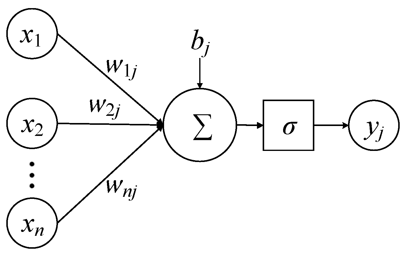
2.1. Deep Learning

As a subclass of machine learning (ML), DL is extensively applied in various social production and practice scenarios. DL evolved from research on artificial neural networks (ANNs), which are a class of models defined by multilayer network architectures. DL learns the effective information hidden between the incoming data of the input layer by constructing a multi-layer neural network, weights and calculates the results, and transmits them to the output layer through the activation function, and then establishes an intricate nonlinear mapping between the input and output. The deep neural network (DNN), serving as the fundamental algorithm of DL, also serves as the basis of deep learning model architectures such as CNN, RNN, and GAN. It is well suited for addressing general data problems without specific structural characteristics, offering strong versatility and generalization capabilities [29]. Hence, this paper adopts DNN. A DNN is mainly composed of three parts: input layer, hidden layer, and output layer, each of which is composed of a certain number of neurons. The schematic diagram of a single neuron is shown in Figure 1. The input of neuron j is x_i, where w_ij is the weight value between the input x_i and neuron j. After the weighted sum is added with the bias value b_j of neuron j, the output y_j of neuron j is ultimately determined by an activation function σ. The activation function imitates the threshold activation characteristics of human brain neurons, introduces nonlinear features into DNN, and enables the transformation from simple linear space to highly nonlinear space [30].

The DNN schematic diagram is shown in Figure 2. DNN employs forward propagation to transfer data into the neural network and learns the effective information hidden between the data transmitted by the input layer through the neural network. The lower-layer neurons receive the input information transmitted by the upper-layer neurons and calculate the weighted results. The error is obtained by the calculation of the backpropagation loss function, and it is passed to the output layer through the activation function. The weights and bias parameters between neurons are continuously adjusted by the optimizer during the process so that the predicted results are infinitely close to the target, and the complex nonlinear mapping from input to output is achieved. In general, DNN is a nonlinear function in nature. Assuming that the selected activation function is σ, the output of the final output layer is y, the total number of layers is l, the output of the hidden layer is a_i (1 < i < l), the weight matrix is W_l, and the bias vector is b_l, and utilizing the matrix form, the formula for the DNN can be expressed as Equation (1):

$$y=\sigma (a_{l-1}{W}_l+b_l)$$

(1)

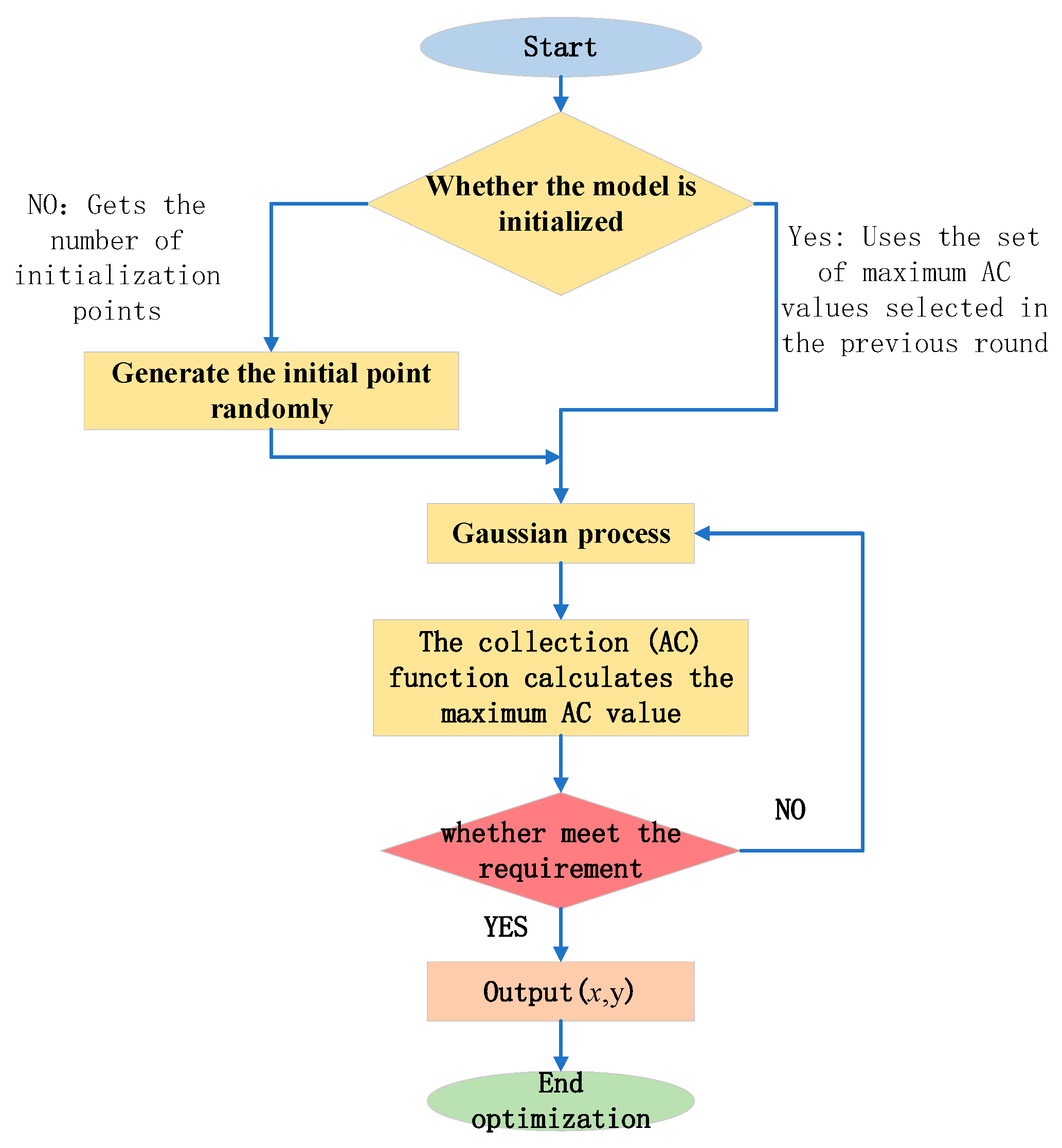
2.2. Bayesian Optimization Algorithm

In general, constructing DNN models requires tuning hyperparameters to obtain an optimal architecture, and the model’s final performance is highly dependent on these parameters. Parameter tuning is a time-consuming and complex task, and it takes a long time to adjust these parameters if the trial-and-error method (manual parameter tuning) is employed. Moreover, the number of hyperparameters and the complexity of the model make it difficult to obtain the optimal parameters by the trial-and-error method, so it is crucial to select an appropriate optimization method to determine the optimal hyperparameters. At present, the prevalent algorithms for hyperparameter optimization include grid search (GS) [31], random search (RS) [32], and Bayesian optimization (BO) [33]. The primary limitation of RS and GS lies in the fact that each computation within their iterations is independent of the previous selection, resulting in significant time wastage during the search for underperforming regions. BO effectively addresses this issue. BO was proposed by Snoek, which is a much more effective tool for DNN such nonlinear function optimization problems. BO determines the next hyperparameter value based on the result of the previous hyperparameter value, which avoids many unnecessary calculations and can find the optimal hyperparameter combination in fewer iterations than GS and RS, so this paper adopts BO to adjust the parameters of the model.

BO optimization primarily comprises two components: a probabilistic surrogate model and an acquisition function. The probabilistic surrogate model represents the distribution of the objective function to be optimized, and the acquisition function is utilized to seek and confirm the next possible extreme point from the posterior distribution. The acquisition function serves two purposes: one is for exploitation, and the other is for exploration. Exploitation is sampling around existing extremes to search for possible better hyperparameter combinations. Exploration is exploring new areas to prevent the optimization from getting trapped in local optima. The primary optimization process is initially generating a probability surrogate model through random sampling and updating the posterior distribution of the objective function (Gaussian process) by continuously adding sample points until the posterior distribution closely approximates the real distribution. In short, this approach considers information from previous parameters to better adjust the current parameter. Its theoretical foundation is based on Bayes’ theorem, as depicted in Equation (2). The flowchart of Bayesian optimization is shown in Figure 3.

$$p\left(f\left|D_{1:t}\right.\right)={\displaystyle \frac{p\left(D_{1:t}\left|f\right.\right)p\left(f\right)}{p\left(D_{1:t}\right)}}$$

(2)

where D_1:t represents the observed data set; p(f|D_1:t) represents the posterior probability; p(D_1:t|f) represents the likelihood distribution probability; p(f) represents the prior probability; and p(D_1:t) represents the marginal likelihood distribution.

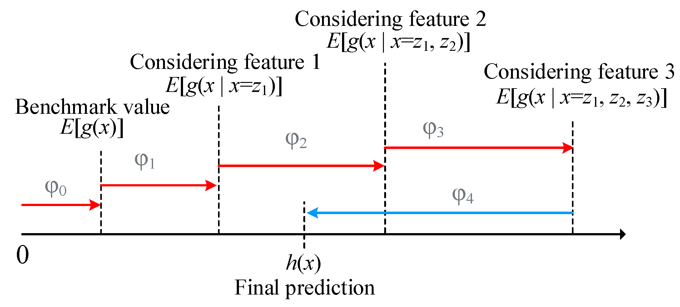
2.3. SHAP Interpretability Method

It is widely known that DL is a “black box” model; that is, such models can give accurate predictions based on inputs but cannot explain the model’s prediction results, which reduces the credibility and application scope of DL models. Therefore, while focusing on improving the performance of the model, it is also important to understand and explain the relationship between input and output. The interpretability of prediction results can be achieved through various methodologies, including but not limited to feature importance, partial dependence plot (PDP) [34], accumulated local effect plot (ALE) [35], and SHAP [36]. Feature importance provides a generalized outcome for the model and quantifies the significance of features by evaluating the prediction error resulting from replacing feature values. However, it does not capture the correlation between features. PDP can express the marginal effect of features on the prediction results at various possible values, but PDP assumes that features are not correlated, which limits the use of PDP. Although ALE solves the problem of correlation between features, the accuracy of ALE depends on the interval range of conditional distribution. SHAP is a game-theory-based approach for interpreting complex ML models. It interprets the model’s output as the sum of contribution values from each input feature, effectively integrating global and local interpretability. Therefore, this paper conducts an interpretability analysis of the prediction results of the model through the SHAP method.

SHAP explains the model by calculating the contribution of each feature when it is added to the model. The sum of all feature contributions determines the model’s final prediction. In accordance with SHAP methodology, the model output is derived from a linear summation of SHAP values associated with input features. Simply put, it quantifies the impact of each input feature on the final output as a specific SHAP value, which can be expressed as:

$$g\left(x^{’}\right)={\phi }_0+{\sum }_{i=1}^N{\phi }_i{x}^{’}$$

(3)

where g(x′) represents the corresponding explanatory model; N represents the total number of features; x represents the input feature; x′ represents the simplified input feature that has a mapping relationship with x, x′⊂{0,1}^N, 1 represents that the feature can be observed, 0 represents that the feature cannot be observed; φ₀ represents the predicted mean value of all samples, that is, the benchmark value; φ_i represents the SHAP value of the i’th feature.

The Shapley value, a concept originally introduced in game theory, measures the contribution of each participant in a cooperative game. The calculation formula of Shapley value is shown in Equation (4).

$${\phi }_i(f,x)={\sum }_{z^{’}\subseteq x^{’}}{\displaystyle \frac{\left|z^{’}\right|!(N-\left|z^{’}\right|-1)!}{N!}}\left[f_x\left(z^{’}\right)-f_x\left({\displaystyle \frac{z^{’}}{i}}\right)\right]$$

(4)

where $f_x\left(z^{’}\right)=f_x\left(h_x\right(z^{’}\left)\right)=E\left[g\left(x\right)\left|z_s\right.\right]$ represents the expected value on the subset z′, N represents the feature set; z′ represents the feature subset.

Figure 4 provides a concise depiction of the SHAP analysis process for obtaining predicted values from the model. In this representation, blue denotes negative feature contributions, while red represents positive feature contributions. Assuming that the i’th sample is x_i, the j’th feature of the i’th sample is x_ij, the predicted value of the model for the sample is y, and the benchmark value of the entire model is φ₀, then the final predicted value of the model with four input features can be expressed as:

$$y={\phi }_0+{\phi }_1+{\phi }_2+{\phi }_3+{\phi }_4$$

(5)

It can be observed that SHAP interprets the model’s final prediction for the sample as the sum of the effects of each feature φ_i, which introduces conditional expectations. Therefore, SHAP can reflect the degree of influence and positive and negative correlation of each feature in each sample, not only providing the importance of input features but also showing how each feature affects the final prediction. The final prediction is obtained by summing the SHAP values φ_i of all input features.

3. Model Construction

3.1. Database Creation and Data Pre-Processing

A reliable and comprehensive database is particularly essential for constructing predictive models. Nikbin [28] collected data from 246 fracture tests and trained an ANN model to predict fracture energy with compressive strength, water–binder ratio, maximum aggregate diameter, and age as input features. However, the database lacks detailed information on specimen dimensions. Many researchers have indicated that to enhance the prediction accuracy for fracture energy, it is necessary to consider additional information about concrete specimens. Therefore, this paper establishes a database that compiles three-point bending test data for concrete beams (the test principle is shown in Figure 5). Each test record contains information on constituent materials, mixture proportions, specimen size, curing age, and fracture energy of concrete. The types of concrete include ordinary concrete, dam concrete, high-strength concrete, and self-compacting concrete. Fiber-reinforced concrete is excluded due to the different behavior of fibers compared to aggregates. The fracture energy in all tests was determined according to the RILEM TC50-FCM [4] recommendations by measuring the load–deflection curve (P-δ) of concrete beams with cut-outs and expressed as the area under the curve, as shown in Equation (6).

$$G_F={\displaystyle \frac{W_0+mg{\delta }_{max}}{T\cdot (W-a_0)}}$$

(6)

where G_F represents the fracture energy; W₀ represents the area under P-δ, as shown in Figure 6; mg represents the dead weight of the beam; δ_max represents the maximum deflection in the beam span; T represents the beam width; W represents the beam height; and a₀ represents the initial notch length.

The experimental data from the database are processed to establish a precise and efficient prediction model. Firstly, the data with missing or duplicated parameters were deleted. Secondly, considering that some parameters are not highly relevant to the prediction target, including all of them as features in model training would increase the model’s complexity and training time and might even reduce its accuracy. Therefore, the parameters in the test data were screened and combined. In previous studies and existing codes, fracture energy is usually predicted by compressive strength, maximum aggregate diameter, and water–binder ratio. Bažant et al. [37] analyzed the fracture energy of concrete with different sizes and discovered that the fracture energy was related to the length of the initial notch on the concrete beam. Hu [38] discovered that the fracture energy depends on the size and geometry of the specimen. In addition, the fracture energy of concrete is also influenced by the aggregate content in concrete [39]. The ligament height (beam height minus initial notch length) is usually considered as the concrete specimen dimensions and has been shown to correlate with the fracture energy of a three-point bending beam specimen [40,41]. In summary, 12 input features were finally determined to predict the fracture energy (G_F), which are beam spacing (S), beam height (W), beam width (T), initial notch length (a₀), ligament height (W-a₀), seam height ratio (a₀/W), span–height ratio (S/W), water–binder ratio (w/b), percentage of coarse aggregates (λ), maximum aggregate diameter (D_max), age (age), and concrete compressive strength (f_c). After processing, 775 test records were selected from the database as the final dataset.

Table 1. Parametric statistical characteristics.

Parameter	Unit	Average	Standard Deviation	Minimum	Maximum
Beam spacing	mm	647	323	95	2200
Beam height	mm	142	75.5	38.1	550
Beam width	mm	91.1	34.4	38.1	240
Initial notch length	mm	53.7	31.8	5	220
Ligament height	-	88.5	9.89	20.4	330
Seam height ratio	-	0.39	0.12	0.05	0.6
Span–height ratio	-	4.73	1.56	0.4	8
Water–binder ratio	-	0.47	0.14	0.2	0.74
Percentage of coarse aggregates	-	0.59	0.1	0	0.97
Maximum aggregate diameter	mm	17	9	1.25	80
Age	d	52	58	7	365
Concrete compressive strength	MPa	48.43	17.24	17.2	115.8
Fracture energy	N/m	146.55	82.77	35.35	584.7

shows the statistical characteristics of the final dataset parameters.

Since the original data are multidimensional and the parameters differ in terms of units and magnitudes, directly using the raw data for model training often results in suboptimal performance. Therefore, feature scaling is applied to eliminate the influence of varying units and magnitudes. The formula for feature scaling is as follows:

$$x^{*}={\displaystyle \frac{x-\mu }{\sigma }}$$

(7)

where x is the original data value; μ is the mean of the data set; σ is the standard deviation; and x^* is the data value after standardization.

3.2. Model Parameter Setting

The main parameters to be adjusted in this paper are the number of hidden layers, the number of neurons, the activation function, the learning rate, the optimizer, the regularization, epochs, and the batch_size.

An insufficient number of hidden layers and neurons may result in underfitting, while excessive values can easily lead to overfitting, thereby degrading the model’s generalization ability. Activation functions help map the nonlinear relationship between inputs and outputs. Common activation functions include sigmoid, tanh, relu, and Lrelu. The learning rate influences the model’s convergence efficiency, which in turn affects the training duration.

The optimizer is a critical component during the training phase. Common optimizers include stochastic gradient descent (SGD), stochastic gradient descent algorithm with momentum (SGDM), root mean square propagation (RMSprop), adaptive moment estimation (Adam), etc. This study directly adopts the Adam optimizer because of its advantages, such as simplicity, efficiency, and automatic adjustment in non-convex optimization problems.

Dropout is a standard regularization technique for deep neural networks. Its main idea is to randomly deactivate a certain proportion of neurons during each training iteration, thereby increasing weight sparsity, enhancing feature diversity, and improving the generalization capability of the network.

One epoch represents one complete forward pass and backward propagation over the entire training dataset. Too few epochs may cause insufficient training, while too many can lead to overfitting. Therefore, this study sets a relatively large number of epochs and employs early stopping to prevent the training process from being adversely affected by the epoch count.

Batch_size refers to the amount of data passed to the model in a single training iteration. A batch_size that is too small can result in slow training and difficulty converging, while a batch_size that is too large requires more epochs to reach the same accuracy but processes the data faster.

The hyperparameters of the model in this paper are determined by the BO algorithm, except for those already specified. The dataset was partitioned randomly into a training set and a test set at an 8:2 ratio, with the former being utilized for parameter determination in the model. In order to avoid the contingency of results caused by random partition of the data set, the current model is evaluated by using the method of five-fold cross validation when parameters are adjusted, and the test set only participates in the validation and evaluation of the final model. The value of hyperparameters in this paper is shown in

Table 2. Value of model hyperparameters.

Parameter	Optimization Scope	Final Value
Number of hidden layers	1~10	6
Number of neurons	1~200	12, 42, 65, 37, 18, 1
Activation function	Relu, tanh, Lrelu	relu
Rate of learning	1, 0.01, 0.001, 0.0001	0.001
Optimizer	-	Adam
Regularization	-	dropout
Epochs	-	1500
Batch_size	1~50	16

.

4. Model Prediction Results and Comparison

4.1. Model Prediction Results

Figure 7 shows the prediction results of the DNN model on the training set and test set, and Figure 8 shows the relative error percentage distribution of the training set and test set. The R² of the model on the training set and test set is 0.973 and 0.953, respectively. Overall, the model exhibits strong predictive performance on both the training and test sets, with most of the data points closely distributed on both sides of y = x, except for a few data points that exhibit high dispersion. Approximately 92% of the prediction results in the training set fall within a range of error of 10%, and roughly 87% of the test set results exhibit a relative error below 10%. The proportion of data points with a relative error within 20% is over 90% for both sets, and only about 6% of the test set results have a relative error exceeding 20%.

4.2. Model Comparison

In order to better demonstrate the performance of the model, three empirical formulas for predicting fracture energy proposed in previous studies and codes were selected for comparison, which are as follows:

(1)

Empirical formula proposed by Bažant [18]:

$$\left\{\begin{array}{l}{G}_f={\alpha }_0{\left({\displaystyle \frac{f_c}{0.051}}\right)}^{0.46}{\left(1+{\displaystyle \frac{d_a}{11.27}}\right)}^{0.22}{\left({\displaystyle \frac{w}{c}}\right)}^{-0.3}\\ G_F=2.5G_f\end{array}\right.$$

(8)

(2)

Empirical formula proposed by CEB-90 [42]:

$$G_F=(0.0469d_a^2-0.5d_a+26){\left({\displaystyle \frac{f_c}{10}}\right)}^{0.7}$$

(9)

(3)

Empirical formula proposed by JSCE [43]:

$$G_F=10\left(d_a\right)0.33(f_c{)}^{0.33}$$

(10)

where G_F represents total fracture energy; G_f represents initial fracture energy; d_a represents maximum particle size of aggregate; f_c represents compressive strength; w/c represents water–cement ratio; α₀ is related to aggregate type when the aggregate type is gravel, α₀ = 1.44; when the aggregate type is round aggregate, α₀ = 1.

The above empirical formulas were used to calculate the test set data, respectively, and the results of each empirical formula and the DNN model prediction results were compared with the test result data as shown in Figure 9. As can be seen from Figure 9, when G_F is less than 200 N/m, the predicted values of the Bažant formula and CEB-90 are in better agreement with the experimental values, while the predicted value of JSCE is on the high side with a large error. When G_F is greater than 200 N/m, the G_F values predicted by the Bažant formula and CEB-90 are generally low, with very large prediction errors, while the values predicted by JSCE are relatively better. However, the G_F predicted by the DNN model is significantly less discrete than the other three empirical formulas, with higher accuracy and stability. It indicates that the DNN model can better predict the fracture energy of concrete than the traditional empirical formulas and has a wider application range.

At the same time, three commonly used model evaluation indexes are selected to evaluate the model performance, which are root mean square error (RMSE), mean absolute error (MAE), and mean percentage error (MAPE). The calculation results are shown in

Table 3. Performance evaluation of each model.

Model	Evaluation Indicators
	RMSE (N/m)	MAPE (%)	MAE (N/m)
DNN	20.45	9.5	14.62
Bažant	97.47	37.71	65.38
CEB-90	88.65	37.48	62.07
JSCE	82.66	60.48	66.31

. Smaller RMSE, MAPE, and MAE values indicate a better model fit and lower prediction errors. It can also be seen from the calculation results of various evaluation indexes that the performance of the DNN model is significantly better than the other three empirical formulas, with lower errors.

5. Interpretability Analysis

5.1. Global Interpretative Analysis

In this section, the interpretability analysis of fracture energy is conducted based on the prediction results of the DNN model, aiming to assess the relative importance of each input parameter and the trend of the influence of the variation of each parameter on the fracture energy. Figure 10 summarizes the SHAP values of all characteristic parameters, which illustrates the SHAP value distribution of sample points corresponding to all features in the dataset and the importance ranking of characteristic parameters. In the figure, the vertical axis represents the input features sorted by contribution importance, and the horizontal axis represents the SHAP value of the feature parameter. Positive and negative represent positive and negative influences on output results. The greater the absolute value, the stronger the influence on the prediction. The color represents the size of the feature values, with blue indicating lower values and red indicating higher values.

As illustrated in Figure 10, the maximum particle size of aggregate is the most important parameter affecting the fracture energy. The larger the aggregate particle size, the larger the SHAP value, and the more obvious the positive impact on the fracture energy. The aforementioned conclusion is also in line with theoretical research, as the bridging mechanism and twisted crack mechanism of coarse aggregate serve as the primary toughening sources for concrete. A larger aggregate particle size results in a more convoluted cracking path and wider fracture area upon failure, thereby leading to a higher fracture energy being attained. The compressive strength is the second most influential factor affecting fracture energy. The SHAP value of compressive strength increases with higher compressive strength, indicating that compressive strength exhibits a positive correlation with fracture energy. The strong correlation between the maximum particle size and compressive strength of aggregates and the fracture energy has been repeatedly proved in various literatures [44], and numerous empirical equations have been established through them. When it is not convenient to do experiments, the value of fracture energy can be obtained according to the empirical relationship between them.

Similarly, the SHAP values of beam height, age, beam width, ligament height, and span exhibit a gradual positive trend with increasing characteristic parameters, indicating that the fracture energy increases with the increase in beam height, age, beam width, ligament height, and span. Water–binder ratio, span–height ratio, and initial crack length show negative effects on fracture energy. However, the proportion of coarse aggregate and the seam height ratio did not clearly show the influence trend on the fracture energy in Figure 10, and the SHAP value of the seam height ratio was mostly distributed near 0, indicating that this characteristic parameter contributed little to the overall model. The seam height ratio, defined as the ratio of a₀ and W, is one of the main size parameters affecting the fracture energy of concrete. However, the outcomes obtained from SHAP analysis are not obvious, which may be caused by the limited range of seam height ratio in the data set, and should be carefully considered in future research endeavors.

5.2. Analysis of the Effect of Material Properties on Fracture Energy

The SHAP value summary in Figure 10 provides a general indication of the influence of each characteristic parameter on fracture energy, but it does not provide a detailed understanding of how specific changes in characteristic parameter values affect fracture energy. Therefore, we draw the SHAP dependency graph for individual features to analyze their impact. Figure 11 plots the dependence of water–binder ratio, proportion of coarse aggregate, maximum particle size of aggregate, age and compressive strength of concrete, additionally, span, beam width and beam height are the geometric parameters of the sample, which will be explained in the subsequent analysis section on fracture energy size effect. In Figure 11, the vertical axis represents SHAP values of characteristic parameters, and the horizontal axis represents the value of the characteristic parameter. Positive and negative represent positive and negative influences on output results, and the larger the absolute value is, the greater the influence is.

As can be seen from Figure 11a, the SHAP value of the maximum particle size of aggregate increases with the increase in particle size, reaching its peak at 20 mm and subsequently stabilizing. When the aggregate particle size is below 15 mm, the SHAP value is negative, which adversely impacts fracture energy, which is also consistent with the majority of test observations. The above phenomenon can be explained as follows: the specific surface area of aggregates with different particle sizes varies, and cracks typically form along the bonding interface layer between aggregate particles and cement mortar. The cement mortar on the surface of smaller-sized aggregates is relatively limited, thereby impacting the bonding strength of the interface layer. When the aggregate particle size increases, the cement mortar wrapped on the aggregate surface increases, increasing the bonding strength between the interface and the fracture energy.

The SHAP value of compressive strength exhibits a nonlinear overall trend, initially increasing and then decreasing with the increase in compressive strength, as depicted in Figure 11b. When the compressive strength exceeds 50 MPa, the increase in SHAP value decreases and starts to decrease after exceeding 80 MPa. Meaning that when the compressive strength value is less than 80 MPa, the higher the compressive strength is, the greater the fracture energy is, and the fracture energy starts to decrease after exceeding 80 MPa. This is due to the fact that the interface structure of high-strength concrete is denser and more consistent than that of ordinary concrete, which is closer to homogeneous material. From the perspective of failure, once the specimen undergoes cracking, the propagation of cracks follows a smooth path with relatively low energy required for failure.

It can be clearly seen from Figure 11c that the SHAP value is basically negative when the water–binder ratio exceeds 0.5, which means that a high water–binder ratio will reduce the value of fracture energy. The water–binder ratio is a fundamental aspect of concrete properties, which significantly influences the hydration process and serves as a reflection of its microstructure. The high water–binder ratio results in an elevated porosity and diminished bond strength within both the matrix and interface transition zone, consequently compromising the compactness of the concrete matrix and the ability of concrete to withstand fracture.

It can be seen from Figure 11e that with the increase in the proportion of coarse aggregate, the SHAP value exhibits an initial increase followed by a decrease. When the proportion of coarse aggregate reaches approximately 0.6, the SHAP value attains its maximum positive magnitude. The fracture energy of concrete will increase when the content of coarse aggregate is increased within a certain range, while keeping the other components unchanged. The main crack of the three-point bending beam develops perpendicular to the direction of the maximum principal stress due to the higher strength of coarse aggregate compared to that of the bonding interface layer. When the content of coarse aggregate increases, the crack needs to pass through a greater number of aggregates, causing it to bypass and expand along their surfaces. Consequently, this leads to an extended and more tortuous path for crack development, requiring increased energy consumption for beam failure and resulting in an increase in fracture energy. When the coarse aggregate content further increases, the cement mortar content will decrease, the mortar layer wrapping the coarse aggregate will become thinner, the distance between coarse aggregates will become closer, the anchorage force of each aggregate will decrease, and the bridging effect of the aggregate will be reduced.

The SHAP value exhibits an initial increase followed by a subsequent decrease with the increase in age, as illustrated in Figure 11d. The early age (before 28 days) has a significant negative effect on the fracture energy, and the fracture energy of the concrete specimens in the late age has an increasing trend with the extension of the age. As universally acknowledged, the enhanced mechanical properties of concrete stem from its hydration process. The gel formed during hydration effectively fills internal defects within the matrix, thereby retarding crack initiation and propagation while enhancing fracture resistance. However, as age increases, the hydration process gradually becomes more sufficient; however, there is no significant improvement in crack resistance, and the growth trend of fracture energy tends to be gentle or even slightly decreased.

5.3. Size Effect Analysis of Fracture Energy

Figure 12 presents the SHAP dependency graph for the geometric feature parameters. It can be clearly seen from Figure 12a that the SHAP value of beam height generally increases with the increase in beam height, and the SHAP value changes little after the height increases to 400 mm. It indicates that when the height of the specimen is less than 400 mm, the fracture energy increases with the increase in the height, and the fracture energy is basically unchanged after the height exceeds 400 mm; that is, there is a significant size effect on the fracture energy within a certain range of specimen height.

As can be seen from Figure 12b, when the beam width is below 100 mm, the SHAP value is basically negative and gradually increases with an increase in beam width, but the increase is slow. The SHAP value exhibits a noticeable increase when the beam width exceeds 100 mm and subsequently stabilizes as the beam width reaches approximately 150 mm. The results generally indicate that the fracture energy exhibits an increasing trend with specimen width, yet when the width exceeds 150 mm, there is essentially no significant size effect observed. Xu Shilang et al. [45] conducted three-point bending tests on beams of different thicknesses and concluded that when the width of the specimen was less than 200 mm, the fracture energy increased with the increase in the specimen width; when the specimen width was greater than 200 mm, the fracture energy remained relatively constant.

As can be seen from Figure 12c, the SHAP value of the span–height ratio decreases with the increase in the span–height ratio. When the span–height ratio is less than 4, there is no significant change in the SHAP value; however, for span–height ratios greater than 4, the SHAP value transitions from positive to negative and decreases as the span–height ratio increases. Overall, the fracture energy decreases as the span–height ratio increases, but the size effect becomes more pronounced when the span–height ratio is greater than 4. The reason for this phenomenon is that when the span–height ratio of the specimen is relatively small, the specimen can be regarded as a deep beam. The behavior of deep beams under load is often governed by shear stress, and crack bands tend to form near the notch, resulting in increased fracture energy. When the span–height ratio of the specimen is relatively large, a single main crack will form after being loaded, resulting in reduced energy required for specimen failure.

Figure 12d shows that with the increase in the seam height ratio of the specimen, the SHAP value shows a tendency of increasing initially and then decreasing, and the SHAP value reaches the peak when the seam height ratio is 0.4. In other words, the fracture energy exhibits an initial increase followed by a subsequent decrease as the seam height ratio increases, and the fracture energy reaches the maximum at approximately 0.4 for the seam height ratio. Because the toughness of the specimen is poor in the case of too a small seam height ratio, making it susceptible to rapid damage under maximum load-bearing conditions, the fracture energy is small. When the seam height ratio increases, the toughness of the specimen is enhanced. Furthermore, apart from type I cracks, the failure process of the specimen may also involve type II and type III cracks, thereby resulting in a corresponding increase in fracture energy. However, excessive seam height ratio results in a diminished effective specimen height, leading to a predominance of type I cracks and reduced fracture energy requirements for specimen failure. It can also be seen from Figure 12d that an increase in the seam height ratio from 0.2 to 0.4 leads to a corresponding enhancement of approximately 5 in the SHAP value, while an increase from 0.4 to 0.6 results in a decrease of around 13 in the SHAP value. This indicates that the size effect of fracture energy becomes more pronounced with the increase in the seam height ratio.

The SHAP value of the ligament height exhibits a noticeable increase as the ligament height value increases, as depicted in Figure 12e. It has been demonstrated that there exists a positive correlation between fracture energy and ligament height, with an evident manifestation of size effect. The reason may be attributed to the tortuous fracture path of concrete specimens during the process of failure, wherein the influence of this tortuosity becomes more pronounced with increasing ligament height, resulting in longer cracking paths and higher fracture energy.

6. Conclusions

Accurate and rapid prediction of fracture energy of concrete holds paramount importance in the realms of concrete structure design and failure analysis. In view of the limitations of existing experimental testing methods—such as being time-consuming, having high result variability, and incurring high overall costs—as well as the limited applicability of empirical formulas, this paper employs the DNN algorithm, known for its strong nonlinear analysis capabilities, and incorporates additional influential factors to enhance the prediction accuracy of the DNN model. The SHAP method is employed to analyze the impact of each parameter on fracture energy and the size effect, based on the predictive results obtained from DNN. The specific conclusions are as follows:

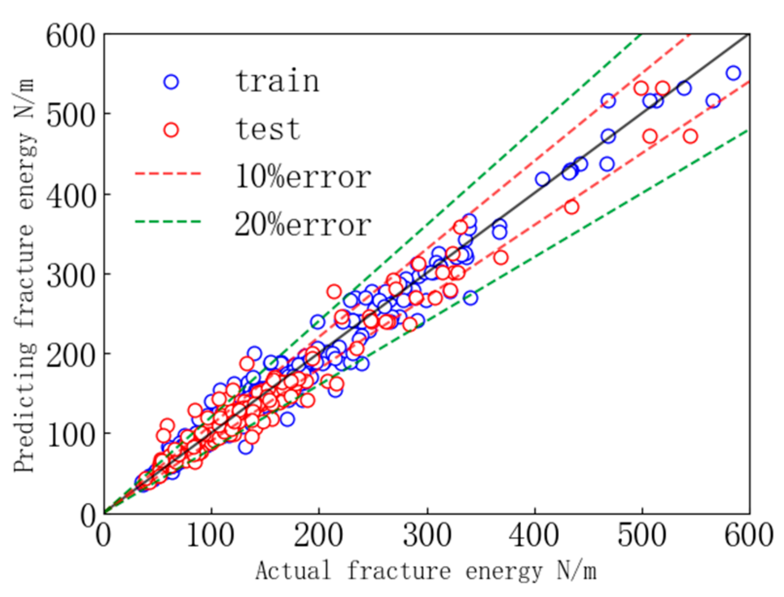
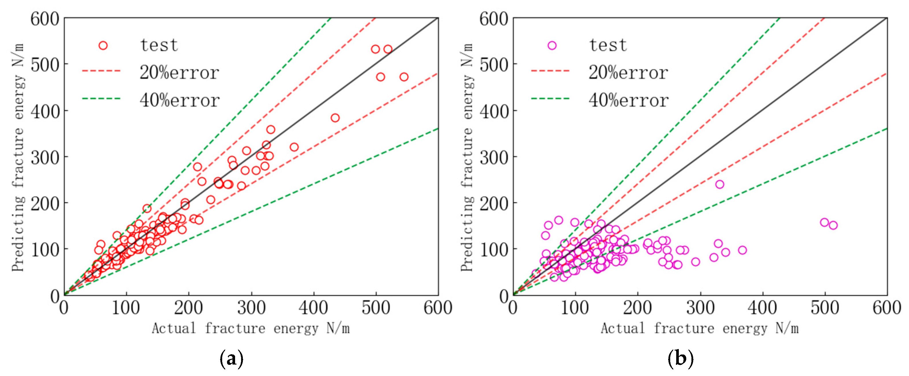
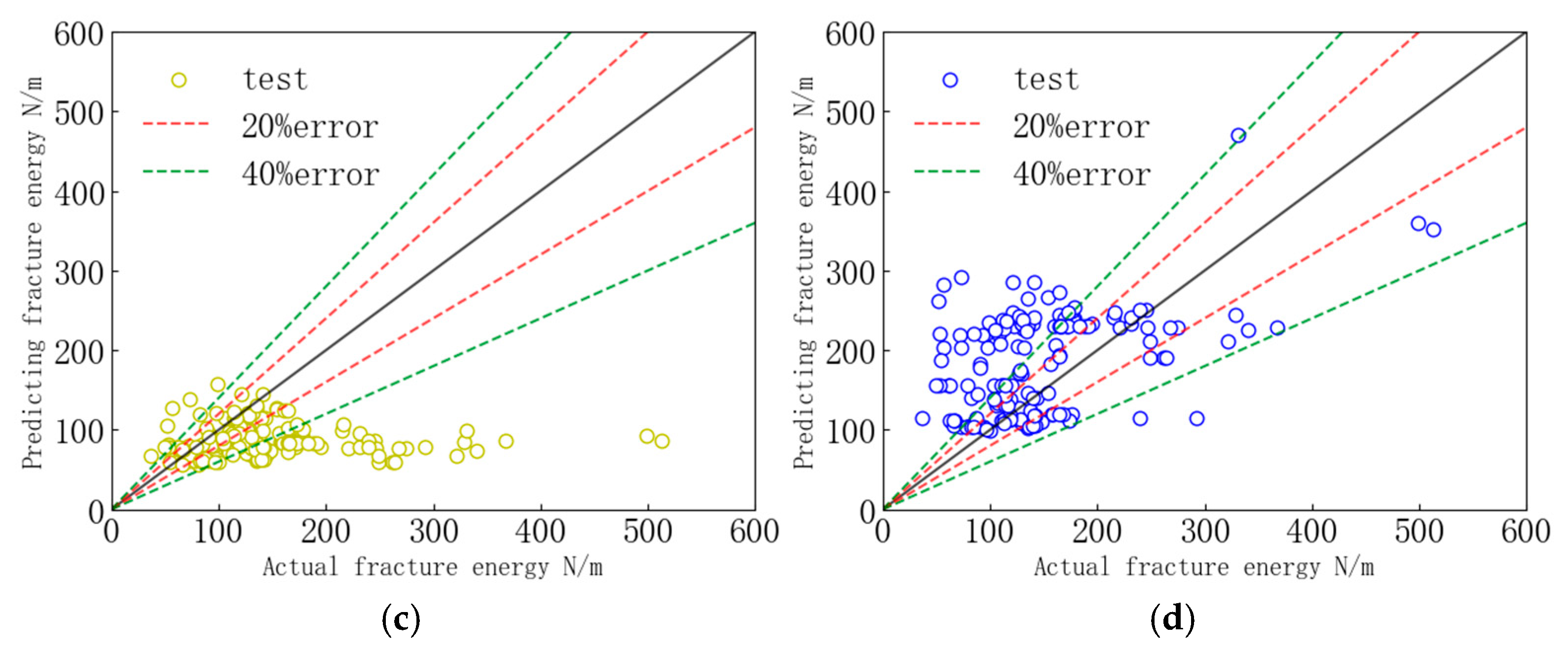
• Development and optimization of DNN model for predicting concrete fracture energy: Firstly, a fracture energy test database was established, followed by the construction of a DNN model based on deep learning for predicting concrete fracture energy. Subsequently, the Bayesian optimization algorithm was employed to obtain an optimal prediction model and accurately predict the fracture energy. The results demonstrate that the predicted values of DNN are in good agreement with the experimental data, with R² being 0.953 and MAPE being 9.5% on the test set. Moreover, the DNN model exhibits superior accuracy and stability compared to existing regression models, expanding its applicability range, which proves that the model in this paper can be used as an effective model to determine the fracture energy of concrete.
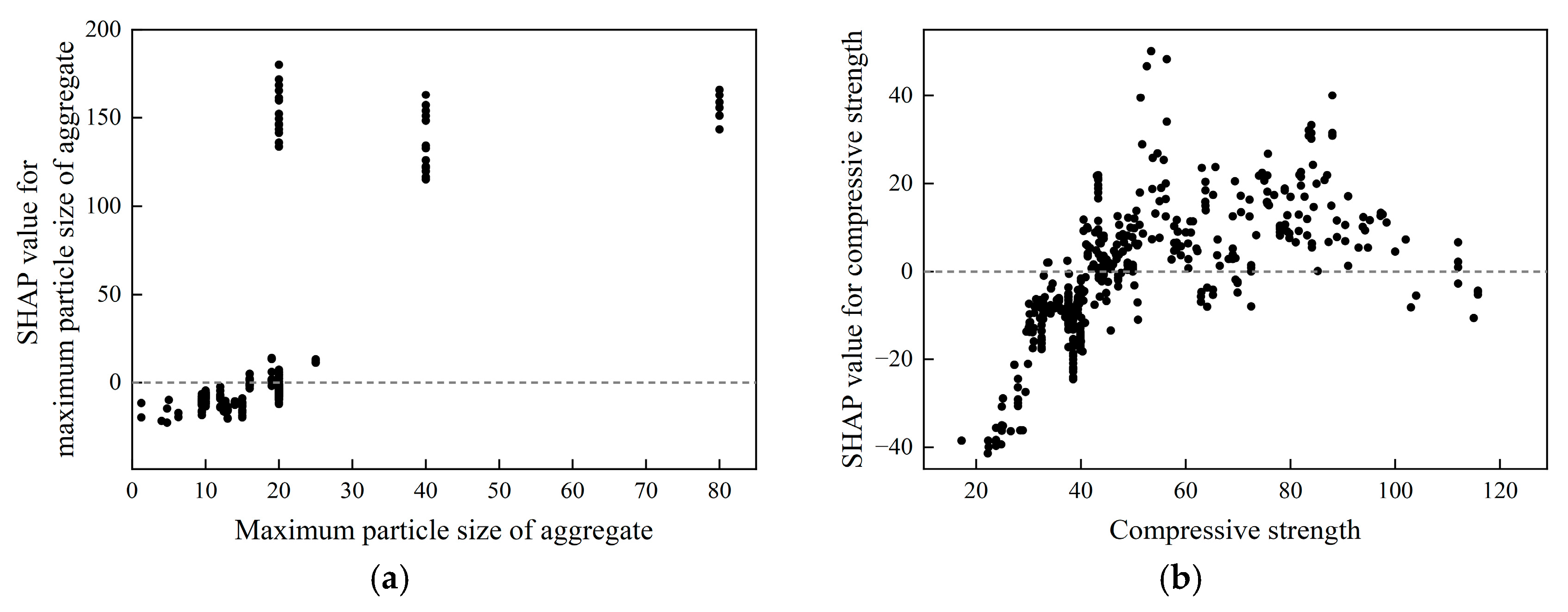
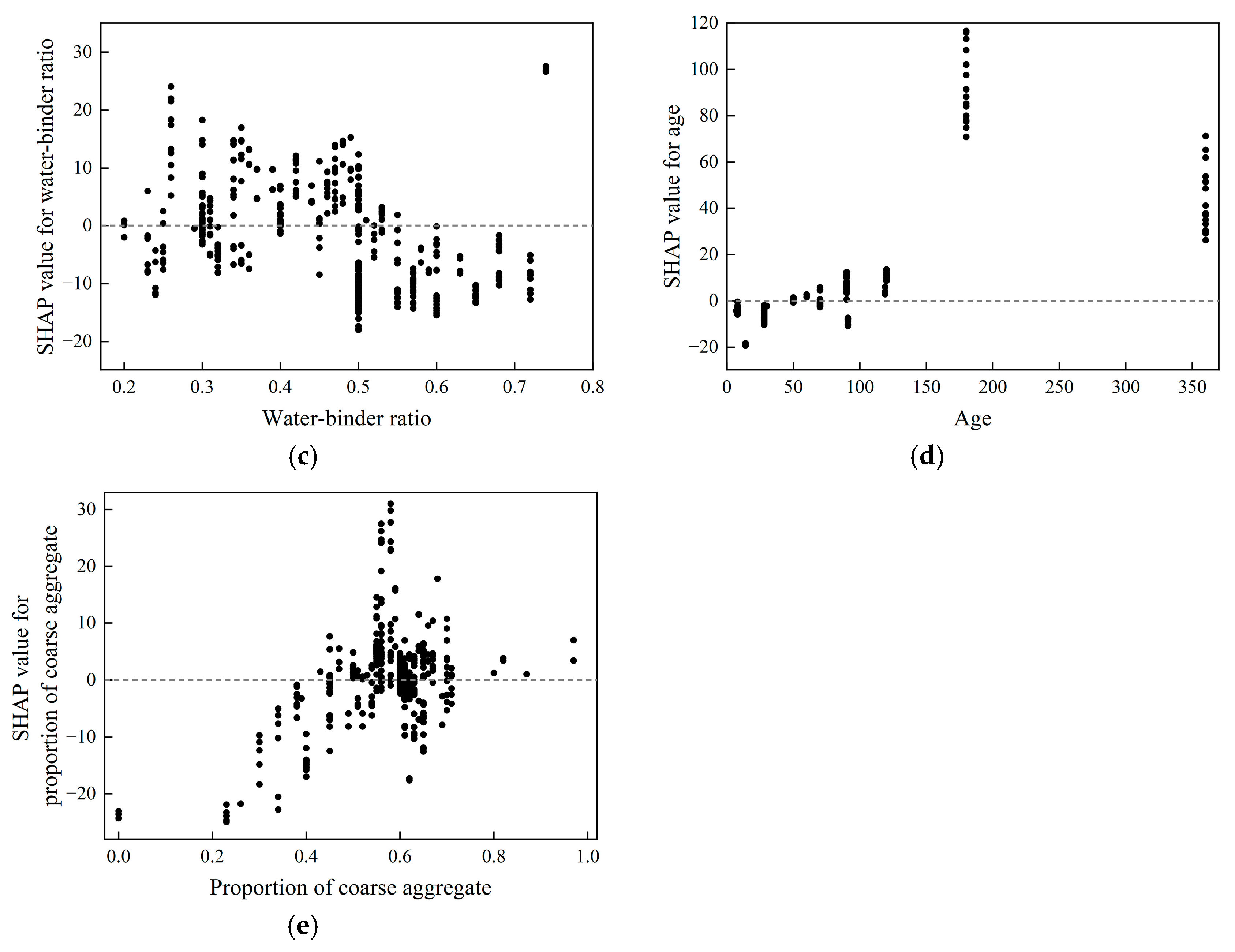
• Feature importance analysis based on SHAP: The significance of each characteristic parameter and how each feature parameter impacts the size of fracture energy are detailedly analyzed by visualizing the SHAP value of the features. The analysis reveals that the fracture energy exhibits an increasing trend with the enlargement of aggregate particle size and tends to stabilize once the particle size exceeds 20 mm; the fracture energy initially rises and then declines as compressive strength increases; a higher water–binder ratio leads to a reduction in fracture energy; the fracture energy demonstrates an initial increase followed by a decrease with an increase in coarse aggregate proportion, reaching its maximum when the proportion is approximately 0.6; and as age progresses, the fracture energy shows a trend of initial increase followed by a decrease.
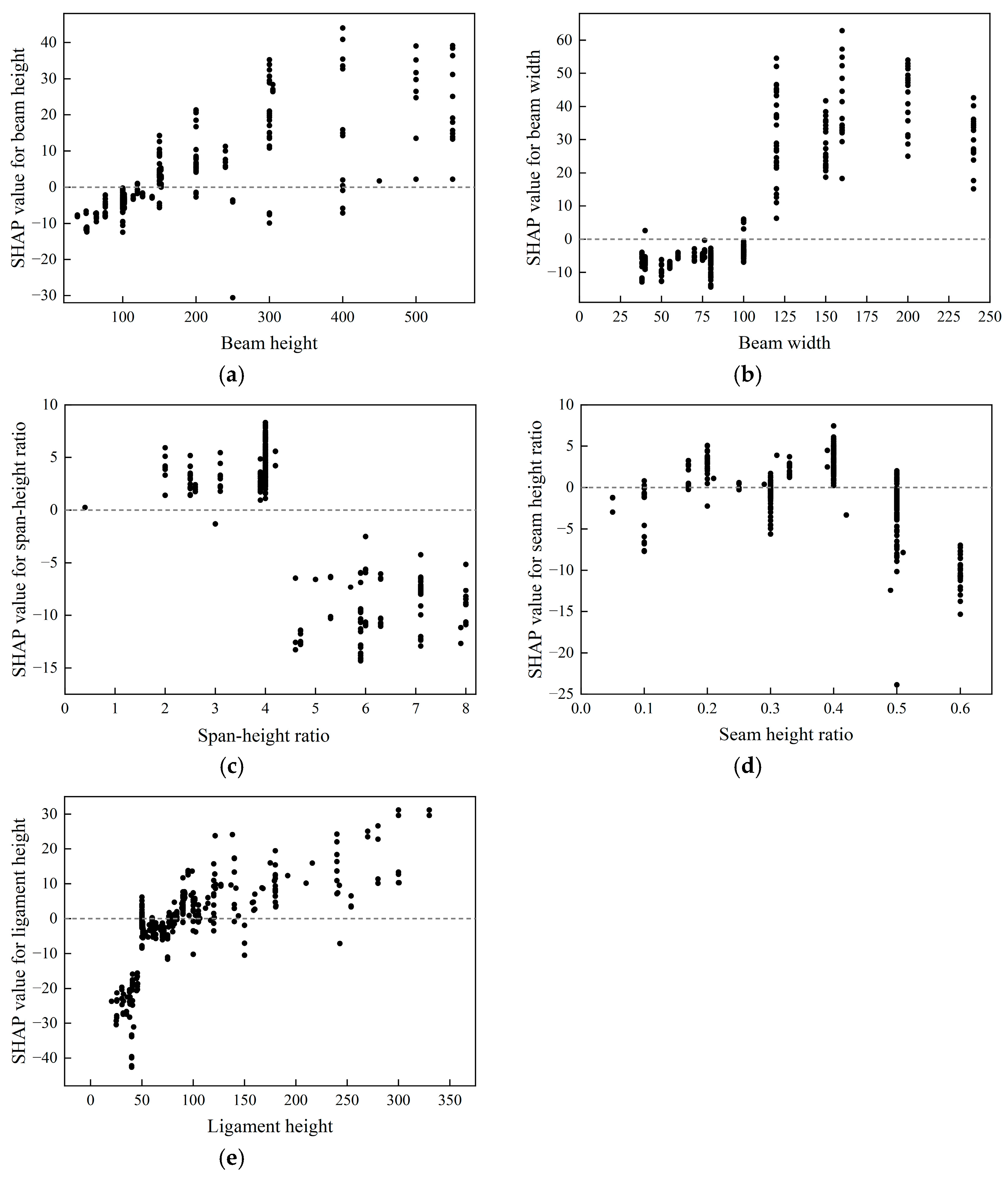
• Size effect analysis of fracture energy based on feature parameter dependence: The size effect of fracture energy in concrete is analyzed in depth by means of a SHAP dependency graph generated by visualization of geometric parameters. The analysis reveals that the fracture energy exhibits an increasing trend with the specimen height, while a decrease in fracture energy is observed when the specimen height exceeds 400 mm, indicating a size effect within a specific range of specimen height; an increase in specimen width leads to an increase in fracture energy, but the increase in width does not cause the size effect after the width exceeds 150 mm; as the span–height ratio increases, there is a decrease in fracture energy, but the size effect becomes more pronounced when the span–height ratio exceeds 4; the fracture energy initially rises and then declines with an increase in seam height ratio until it reaches its maximum at approximately 0.4; there exists a positive correlation between fracture energy and ligament height with the evident size effect.

While this study has demonstrated the effectiveness of a DNN framework integrated with the SHAP interpretability method in predicting the fracture energy of concrete and has explored the influence of size effects, certain limitations remain and warrant further investigation. The main aspects are as follows:

• Concrete, as a typical multiphase composite material, exhibits complex mechanical behavior due to its heterogeneous composition. This study examined the influence of multiple feature parameters on concrete fracture energy; however, the synergistic effects among features have not yet been quantified. A deeper analysis of feature interrelationships may facilitate the development of more comprehensive predictive models.
• The study was constrained by the number of input features and the size of the dataset. Future work incorporating more extensive and diverse datasets, along with a broader range of concrete parameters, may lead to the construction of a more robust and inclusive prediction model.
• Given the diversity of current deep learning architectures, integrating more advanced and powerful models may improve both prediction accuracy and interpretability, thus providing more reliable guidance for engineering applications.

References

1. Hadjari, M.; Marouf, H.; Dahou, Z.; Maherzi, W. Investigation of the Mechanical and Fracture Properties of Recycled Aggregate Concrete. Buildings 2025, 15, 1155. [Google Scholar] [CrossRef]
2. Nikbin, I.M.; Davoodi, M.R.; Fallahnejad, H.; Rahimi, S.; Farahbod, F. Influence of mineral powder content on the fracture behaviors and ductility of selfcompacting concrete. J. Mater. Civ. Eng. 2015, 28, 4015147. [Google Scholar] [CrossRef]
3. Beygi, M.H.; Kazemi, M.T.; Amiri, J.V.; Nikbin, I.M.; Rabbanifar, S.; Rahmani, E. Evaluation of the effect of maximum aggregate size on fracture behavior of self compacting concrete. Constr. Build. Mater. 2014, 55, 202–211. [Google Scholar] [CrossRef]
4. RILEM. Draft recommendation TC50-FCM:Determinationof fracture energy of mortar and concrete by means of three-Point bend tests on notched beams. Mater. Struct. 1985, 18, 285–290. [Google Scholar]
5. DL/T 5332−2005; Code for Fracture Test of Hydraulic Concrete of National Development and Reform Commission of the People’s Republic of China. China Electric Power Press: Beijing, China, 2006.
6. Dong, L.; Liu, J.; Xiu, L.D.; Jing, B.L. A theoretical method to determine the tortuous crack length and the mechanical parameters of concrete in direct tension-A particle size effect analysis. Eng. Fract. Mech. 2018, 197, 128–150. [Google Scholar]
7. Hu, S.; Fan, B. Study on the bilinear softening mode and fracture parameters of concrete in low temperature environments. Eng. Fract. Mech. 2019, 211, 1–16. [Google Scholar] [CrossRef]
8. Rong, H.; Dong, W.; Zhang, X.; Zhang, B. Size effect on fracture properties of concrete after sustained loading. Mater. Struct. 2019, 52, 16. [Google Scholar] [CrossRef]
9. Bakour, A.; Ftima, M.B. Investigation of fracture properties and size effects of mass concrete using wedge splitting tests on large specimens. Eng. Fract. Mech. 2022, 259, 108144. [Google Scholar] [CrossRef]
10. Sun, L.; Du, C.; Ghaemian, M.; Zhao, W. Determination of the fracture parameters of concrete with improved wedge-splitting testing. Eng. Fract. Mech. 2022, 276, 108911. [Google Scholar] [CrossRef]
11. Lei, Y.; Jin, L.; Du, X. Experimental investigation of size effects on BFRP-RC beams under combined bend-ing-shear-torsion loading. Eng. Struct. 2025, 336, 120457. [Google Scholar] [CrossRef]
12. Jia, P.; Wu, H.; Ma, L. Size effect for dynamic flexural responses of RC beams under low-velocity impact. Eng. Struct. 2025, 338, 120598. [Google Scholar] [CrossRef]
13. Zhao, Z.; Kwon, S.H.; Shah, S.P. Effect of specimen size on fracture energy and softening curve of concrete: Part I. Experiments and fracture energy, Cem. Concr. Res. 2008, 38, 1049–1060. [Google Scholar] [CrossRef]
14. Zong, Y. Experimental Study on Wedge Splitting Tensile Fracture of Fully-Graded Concrete. Master’s Thesis, Kunming University of Science and Technology, Kunming, China, 2018. [Google Scholar]
15. Carloni, C.; Santandrea, M.; Baietti, G. Influence of the Width of the Specimen on the Fracture Response of Concrete Notched Beams. Eng. Fract. Mech. 2019, 216, 7–10. [Google Scholar] [CrossRef]
16. Duan, K.; Hu, X.Z.; Wittmann, F.H. Thickness Effect on Fracture Energy of Cementitious Materials. Cem. Concr. Res. 2003, 33, 499–507. [Google Scholar] [CrossRef]
17. Elices, M.; Rocco, C. Effect of aggregate size on the fracture and mechanical properties of a simple concrete. Eng. Fract. Mech. 2008, 75, 3839–3851. [Google Scholar] [CrossRef]
18. Bažant, Z.P.; Becq-Giraudon, E. Statistical prediction of fracture parameters of concrete and implications for choice of testing standard. Cem. Concr. Res. 2002, 32, 529–556. [Google Scholar] [CrossRef]
19. Hu, S.W.; Mi, Z.X.; Lu, J.; Fan, X.-Q. A study on energy dissipation of fracture process zone in concrete. J. Hydraul. Eng. 2012, 43, 145–152. [Google Scholar]
20. Yin, Y.; Qiao, Y.; Hu, S. Determining concrete fracture parameters using three-point bending beams with various specimen spans. Theor. Appl. Fract. Mech. 2020, 107, 102465. [Google Scholar] [CrossRef]
21. Xie, J.; Liu, Y.; Yan, M.-L.; Yan, J.-B. Mode Ⅰ fracture behaviors of concrete at low temperatures. Constr. Build. Mater. 2022, 323, 126612. [Google Scholar] [CrossRef]
22. Silva, W.R.L.D.; Lucena, D.S.D. Concrete Cracks Detection Based on Deep Learning Image Classification. Proceedings 2018, 2, 489. [Google Scholar] [CrossRef]
23. Deng, F.; He, Y.; Zhou, S.; Yu, Y.; Cheng, H.; Wu, X. Compressive strength prediction of recycled concrete based on deep learning. Constr. Build. Mater. 2018, 175, 562–569. [Google Scholar] [CrossRef]
24. Zhou, S.; Sheng, W.; Wang, Z.; Yao, W.; Huang, H.; Wei, Y.; Li, R. Quick image analysis of concrete pore structure based on deep learning. Constr. Build. Mater. 2019, 208, 144–157. [Google Scholar] [CrossRef]
25. Latif, S.D. Concrete compressive strength prediction modeling utilizing deep learning long short-term memory algorithm for a sustainable environment. Environ. Sci. Pollut. Res. 2021, 28, 30294–30302. [Google Scholar] [CrossRef] [PubMed]
26. Ince, R. Prediction of fracture parameters of concrete by Artificial Neural Networks. Eng. Fract. Mech. 2004, 71, 2143–2159. [Google Scholar] [CrossRef]
27. Yan, Y.; Ren, Q.; Xia, N.; Shen, L.; Gu, J. Artificial neural network approach to predict the fracture parameters of the size effect model for concrete. Fatigue Fract. Eng. Mater. Struct. 2015, 38, 1347–1358. [Google Scholar] [CrossRef]
28. Nikbin, I.M.; Rahimi, S.; Allahyari, H. A new empirical formula for prediction of fracture energy of concrete based on the artificial neural network. Eng. Fract. Mech. 2017, 186, 466–482. [Google Scholar] [CrossRef]
29. An, P.; Cao, D.P.; Zhao, B.Y.; Yang, X.L.; Zhang, M. Reservoir physical parameters prediction based on LSTM recurrent neural network. Prog. Geophys. 2019, 34, 1849–1858. [Google Scholar]
30. Tian, R.; Meng, H.; Chen, S.; Wang, C.; Zhang, F. Prediction of intensity classification of rockburst based on deep neural network. J. China Coal Soc. 2020, 45, 191–201. [Google Scholar]
31. Bergstra, J.; Bardenet, R.; Bengio, Y.; Kégl, B. Algorithms for hyper-parameter optimization. In Proceedings of the 24th International Conference on Neural Information Processing Systems, Vancouver, BC, USA, 6–9 December 2010; Curran Associates Inc.: Red Hook, NY, USA, 2011; pp. 2546–2554. [Google Scholar]
32. Bergstra, J.; Bengio, Y. Random search for hyper-parameter optimization. J. Mach. Learn. Res. 2012, 13, 281–305. [Google Scholar]
33. Snoek, J.; Larochelle, H.; Adams, R.P. Practical Bayesian optimization of machine learning algorithms. In Proceedings of the 25th International Conference on Neural Information Processing Systems, Lake Tahoe, NV, USA, 3–6 December 2012; ACM: New York, NY, USA, 2012; Volume 2, pp. 2951–2959. [Google Scholar]
34. Friedman, J.H. Greedy function approximation: A gradient boosting machine. Ann. Stat. 2001, 29, 1189–1232. [Google Scholar] [CrossRef]
35. Apley, D.W.; Zhu, J. Visualizing the Effects of Predictor Variables in Black Box Supervised Learning Models. arXiv 2016, arXiv:1612.08468. [Google Scholar] [CrossRef]
36. Lundberg, S.M.; Lee, S.I. A unified approach to interpreting model predictions. Adv. Neural Inf. Process. Syst. 2017, 30, 4765–4774. [Google Scholar]
37. Bažant, Z.P.; Kazemi, M.T. Size dependence of concrete fracture energy determined by RILEM work-of-fracture method. Int. J. Fract. 1991, 51, 121–138. [Google Scholar] [CrossRef]
38. Hu, X.Z. An asymptotic approach to size effect on fracture toughness and fracture energy of composites. Eng. Fract. Mech. 2002, 69, 555–564. [Google Scholar] [CrossRef]
39. Vishalakshi, K.P.; Revathi, V.; Sivamurthy Reddy, S. Effect of type of coarse aggregate on the strength properties and fracture energy of normal and high strength concrete. Eng. Fract. Mech. 2018, 194, 52–60. [Google Scholar] [CrossRef]
40. Duan, K.; Hu, X.Z.; Wittmann, F.H. Size effect on specific fracture energy of concrete. Eng. Fract. Mech. 2007, 74, 87–96. [Google Scholar] [CrossRef]
41. Guan, J.F.; Hu, X.Z.; Li, Q.B. In-depth analysis of notched 3-p-b concrete fracture. Eng. Fract. Mech. 2016, 165, 57–71. [Google Scholar] [CrossRef]
42. Comite Euro-lnternational Du Beton. CEB-FIP Model Code 1990; Thomas Telford Publishing: London, UK, 1993. [Google Scholar]
43. Japan Society of Civil Engineers. Standard Specifications for Concrete Structures 2007 “Design”; Japan Society of Civil Engineers: Tokyo, Japan, 2010. [Google Scholar]
44. Mazloom, M.; Salehi, H. The relationship between fracture toughness and compressive strength of self-compacting lightweight concrete. IOP Conf. Ser. Mater. Sci. Eng. 2018, 431, 062007. [Google Scholar] [CrossRef]
45. Xu, S.L.; Zhao, G.F.; Liu, Y.; Ye, L.D. The three-point bending beam method is used to study the fracture energy of concrete and the influence of specimen size. J. Dalian Univ. Technol. 1991, 79–86. [Google Scholar]
Figure 1. Single neuron.
Buildings 15 02149 g001
Figure 2. Schematic diagram of DNN.
Buildings 15 02149 g002
Figure 3. The flowchart of Bayesian optimization.
Buildings 15 02149 g003
Figure 4. Schematic diagram of interpretation of SHAP additivity.
Buildings 15 02149 g004
Figure 5. Schematic diagram of three-point bending test.
Buildings 15 02149 g005
Figure 6. P-δ curve.
Buildings 15 02149 g006
Figure 7. DNN model prediction results.
Buildings 15 02149 g007
Figure 8. Relative error distribution of prediction results.
Buildings 15 02149 g008
Figure 9. Comparison chart of prediction results of DNN model and empirical formula with test data: (a) DNN; (b) Bažant [18]; (c) CEB-90 [42]; (d) JSCE [43].
Buildings 15 02149 g009aBuildings 15 02149 g009b
Figure 10. Summary chart of SHAP values.
Buildings 15 02149 g010
Figure 11. SHAP feature dependency graph: (a) SHAP value variation of maximum particle size of aggregate; (b) SHAP value variation of compressive strength; (c) SHAP value variation of water–binder ratio; (d) SHAP value variation of age; (e) SHAP value variation of proportion of coarse aggregate.
Buildings 15 02149 g011aBuildings 15 02149 g011b
Figure 12. SHAP feature dependency graph: (a) SHAP value variation of beam height; (b) SHAP value variation of beam width; (c) SHAP value variation of span–height ratio; (d) SHAP value variation of seam height ratio; (e) SHAP value variation of ligament height.
Buildings 15 02149 g012