A Point Cloud Registration Method for Steel Tubular Arch Rib Segments of CFST Arch Bridges Based on Local Geometric Constraints

Abstract

The multi-station registration of concrete-filled steel tubular (CFST) arch rib segments poses significant challenges due to structural complexity and environmental constraints during terrestrial laser scanning, requiring multi-angle acquisition for comprehensive coverage. This study introduces a cascaded registration framework comprising: (1) a coarse registration method utilizing local geometric features of segmented tubular joints, where equidistant cross-section partitioning extracts inherent circularity constraints from cylindrical segments, and (2) a refined registration stage employing the Coherent Point Drift (CPD) algorithm with k-d tree acceleration for computational efficiency. Experimental results demonstrate that the coarse registration achieves 31 mm RMSE with R²= 0.889, eliminating 88.9% of initial misalignment. The CPD refinement reduces RMSE to 4 mm (87% precision improvement), reaching sub-centimeter accuracy with exceptional congruence (R² = 0.995, residual error = 0.5%). Notably, k-d tree acceleration decreases computational time by 34.2% (13.30 s vs. 20.21 s) compared to conventional CPD. Validated on 2.2 m CFST specimens, this method provides an efficient solution for multi-station point cloud registration of complex steel structures.

1. Introduction

Concrete-filled steel tubular (CFST) arch bridges represent a composite structure where steel tubes are filled with concrete to form the main arch ribs. This configuration synergistically combines the compressive strength of concrete with the tensile resistance of steel tubes, leading to widespread adoption in highway, railway, and urban bridge construction [1]. The fabrication process involves steel plate cutting, tube rolling, joint alignment, and on-site assembly. Precise dimensional control during prefabrication requires rigorous metrological verification of arch rib components.

However, the geometrically complex spatial configuration and large dimensions of CFST arch ribs (typically exceeding 50 m span) pose significant challenges to conventional measurement techniques. Total stations and theodolites are constrained to discrete point measurements, exhibiting limited spatial coverage (generally <85% surface mapping) and positioning accuracy (±3–5 mm at 50 m distance). Although the GPS demonstrates advantages in large-scale positioning (±2 cm accuracy), its applicability diminishes in capturing intricate component features due to inherent signal multipath effects in steel structures. Photogrammetry enables partial 3D reconstruction but demands specialized operators and incurs high computational costs (typically >USD1500/m³ point cloud processing) [2,3]. Terrestrial laser scanning (TLS) has emerged as a transformative geospatial technology, achieving point cloud densities up to 1 million points/sec with ±2mm accuracy. Beyond topographic mapping applications [4,5,6], TLS proves particularly valuable for bridge component measurement through its non-contact, high-fidelity data capture capabilities [7]. In prefabrication yard environments, TLS deployment for CFST arch rib scanning necessitates multi-station configurations (typically 8–12 stations per 10m segment) to overcome occlusions and viewing angle constraints. This multi-view approach generates comprehensive point cloud datasets (>50 million points per rib) essential for full-component characterization and downstream structural analysis. Such high-precision geometric data, when synergized with advanced structural health monitoring models, can establish a static-dynamic fusion analytical basis for lifecycle condition assessment of bridges [8,9].

While multi-station scanning enables full component coverage, it introduces critical challenges in point cloud registration due to coordinate system discrepancies across scanning positions. Accurate alignment of these discrete coordinate frames constitutes a prerequisite for dimensional metrology and deformation analysis. The registration accuracy directly determines the validity of digital pre-assembly outcomes, where aligned point clouds can replace physical trial assemblies to achieve millimeter-level spatial matching (≤0.5 mm tolerance) between segments. This virtual assembly paradigm reduces construction cycles by 40–60% and decreases heavy lifting operations by 75%, while mitigating cumulative measurement errors inherent in field trials. However, suboptimal registration accuracy (>2 mm root mean square error (RMSE)) may lead to catastrophic misinterpretations of structural conditions, as evidenced by the 2018 Quebec bridge retrofit incident [10]. Previous studies have explored various registration strategies. Chang et al. [11] used pre-installed targets to generate feature points for registration in segment assembly research, achieving satisfactory results but introducing errors during feature extraction.

Xu et al. [12] proposed a segmentation-based registration algorithm that combines curvature histogram matching and affine invariant constraints to achieve fast and accurate alignment of large-scale point clouds. Leitenstern M et al. [13] proposed a method integrating keyframe interpolation for automatic point cloud map registration. While this approach eliminates the need for manual targets and enables real-time processing, it relies on GNSS signals and requires significant computational resources. Ji et al. [14] systematically analyzed factors such as target-to-scanner distance and target types, concluding that increasing target quantity and reducing scanning distance improve registration accuracy. Yang et al. [15] proposed an indoor point cloud registration method utilizing local neighborhood features, yet their reliance on labeled transformation matrices limited algorithm applicability. These target-dependent methods predominantly focus on artificial references, overlooking the potential of intrinsic geometric characteristics. Fu Yao et al. [16] proposed a 4PCS+SICP combined algorithm for rail wear measurement, eliminating target dependency by leveraging intrinsic rail point cloud features. However, this method is confined to regular geometries like rails and lacks validation in complex registration scenarios. Sun Wei et al.’s [17] contour-based laser registration improved Iterative Closest Point (ICP) efficiency by 14× (processing time: 72.39 s vs. 5.57 s) maintaining data reproducibility, though requiring pristine surface conditions rarely encountered in construction sites, where components often exhibit welding spatters or surface irregularities. Liu’s et al.’s [18] road scene registration strategy reduced alignment errors by 50% through geographic entity recognition, yet its 38 mm accuracy fails to meet industrial-grade standards for bridge components (typically requiring ≤0.5 mm tolerance) and is unsuitable for large-scale free-form structures with complex spatial geometries. For large-scale free-form surfaces—defined as components with continuous, non-uniform spatial curvature variations (e.g., CFST arch ribs with variable radius of curvature ≥ 5 m)—current algorithms face dual challenges: (1) inadequate characterization of complex curvature (mean curvature error > 0.15 m⁻¹), and (2) precision limitations (5 mm RMSE) exceeding industrial tolerances for mega-structures. This comprehensive review reveals persistent challenges in target-free registration for large-scale free-form structures like CFST arch ribs: (1) Current algorithms developed for regular geometries (e.g., cubes, cylinders) exhibit inadequate characterization of continuous spatial curvature variations, and (2) precision limitations, which exceed the ≤0.5 mm tolerance required for free-form surface components in megastructures (ISO 2768-1:1989 [19] fine class).

This study addresses multi-station registration challenges for large-scale cylindrical joint point clouds by proposing: (1) a coarse registration method constrained by local geometric features of tubular joints, and (2) a refined alignment using the Coherent Point Drift (CPD) algorithm. This hierarchical approach aims to enhance overall registration accuracy while maintaining computational efficiency. Experimental validation demonstrates the method’s effectiveness, providing a referential framework for engineering applications in bridge component measurement and related research domains.

2. Methods and Data

2.1. Point Cloud Registration Method for Arch Rib Joints of CFST Arch Bridges Using 3D Laser Scanning

As illustrated in Figure 1, the proposed registration workflow comprises three stages:

(1)

Point cloud preprocessing: Raw point clouds undergo noise removal and preliminary classification to isolate structural features of the arch rib segments.

(2)

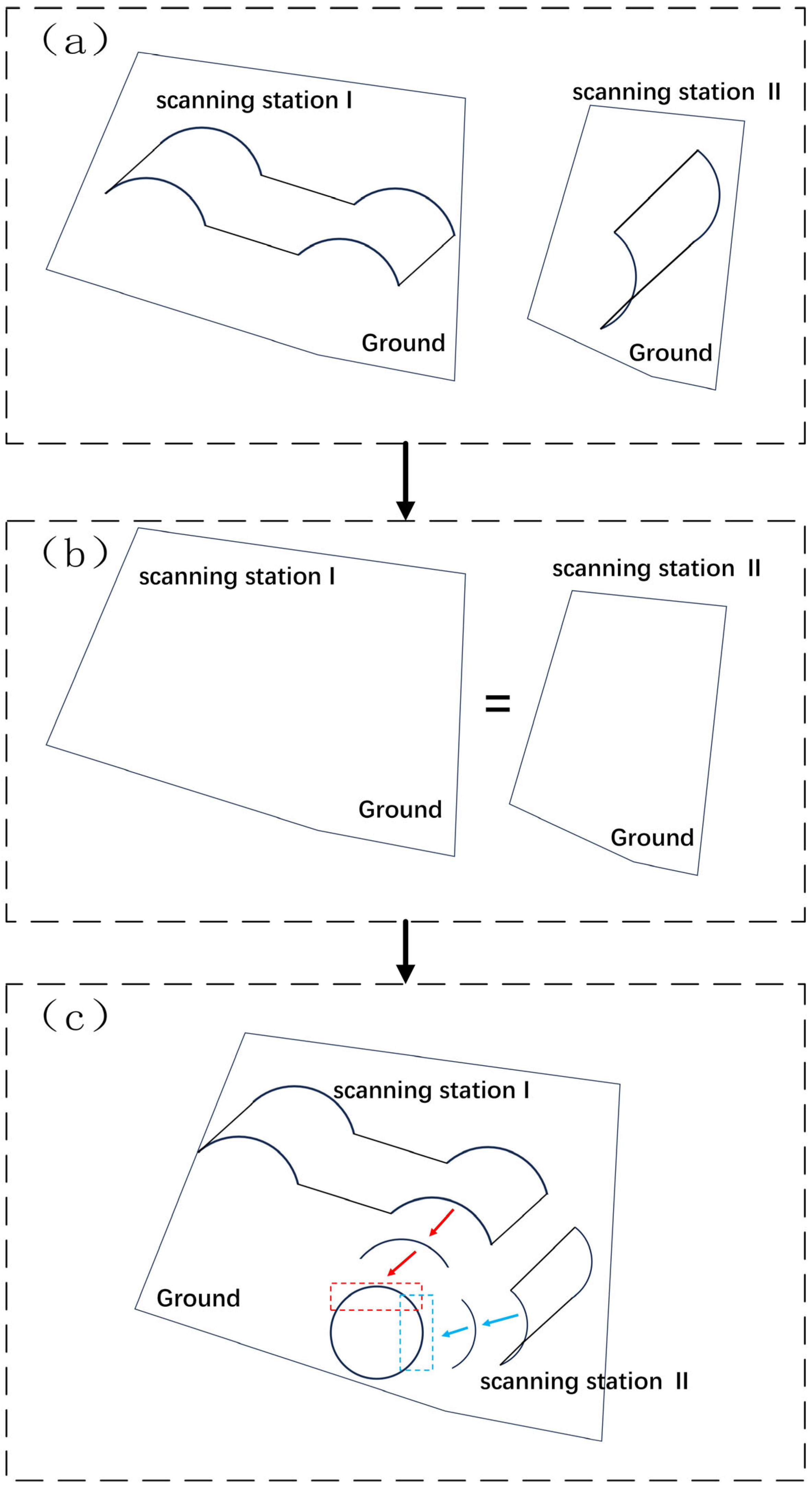
Coarse registration via equidistant partitioning: A novel equidistant partitioning method is applied to segment the multi-station point clouds. The partitioned sub-clouds exhibit regular circular geometries derived from the tubular joints. These geometric invariants are exploited as positional constraints to align point clouds from different scanning stations.

(3)

Fine registration with the CPD algorithm: The coarsely aligned point clouds are further refined using the CPD algorithm. This probabilistic approach iteratively maximizes the spatial coherence between corresponding points, improving registration accuracy.

2.2. Data Preprocessing

Terrestrial laser scanning (TLS) captures comprehensive point cloud data, yet the raw datasets inevitably contain measurement noise (σ ≥ 0.8 mm) and extraneous elements. In this study focusing on geometric feature-based registration of arch rib segments, only data reflecting the primary structural geometry are considered valid. Traditional monolithic preprocessing methods (e.g., basic filtering, downsampling) struggle to efficiently and effectively remove extraneous data while preserving critical geometric features. To address this limitation, we implement a hybrid preprocessing strategy (see Figure 2) comprising three key phases:

• Noise Suppression.
  Initial denoising employs conventional filtering to eliminate obvious outliers while retaining structural contours. For example, median filtering with a window size of 5 × 5 × 5 voxels is used to remove obvious isolated points, followed by Gaussian filtering with a standard deviation (σ) set to 0.5 to further smooth continuous noise.
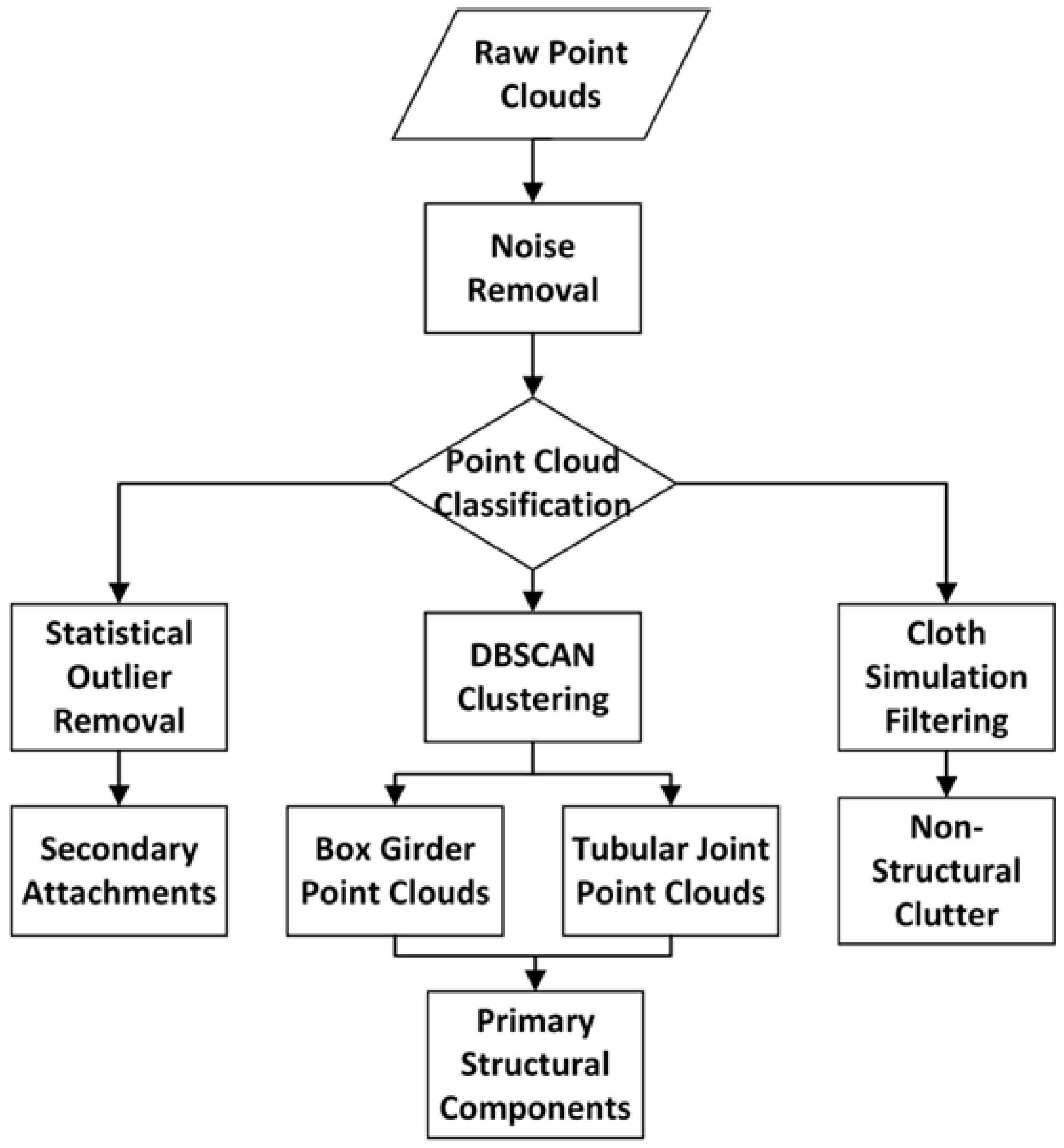
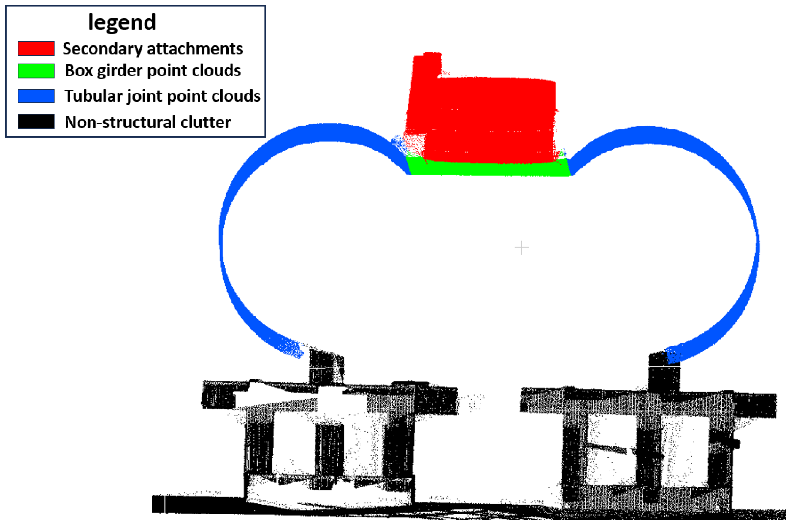
• Component-Wise Classification.
  The sanitized point cloud undergoes feature-based segmentation into three distinct categories:
  • Primary structural components: arch rib segments; box girders.
  • Secondary attachments: non-structural elements.
  • Non-structural clutter: environmental obstructions (detailed taxonomy shown in Figure 3).
• Feature-Specific Processing.
  A multi-algorithm cascade ensures optimal treatment for each category:

  a.

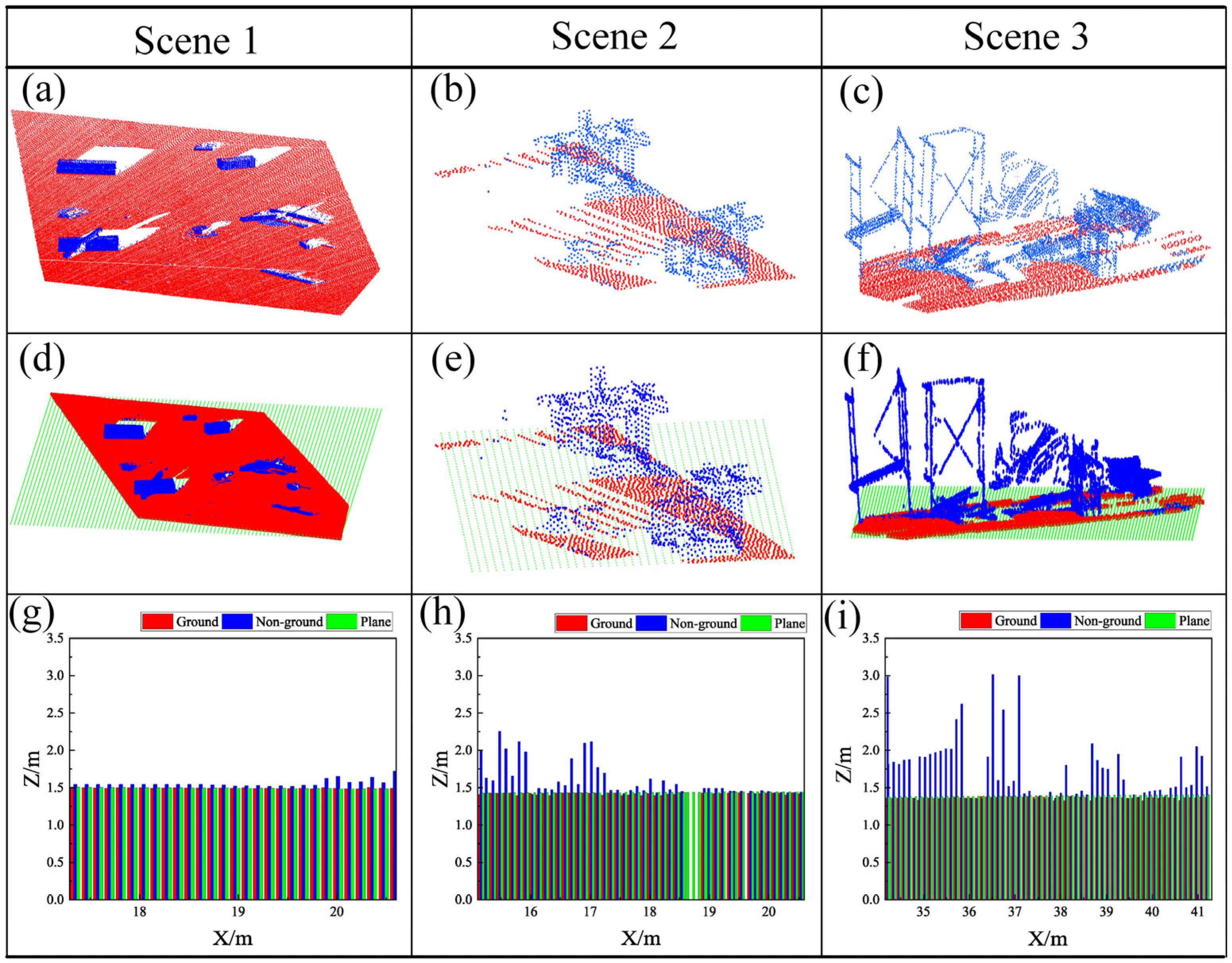
  Cloth Simulation Filtering (CSF) [20]: this physics-based method simulates virtual cloth draping over point cloud surfaces, differentiating the following:

  • Structural points (cloth-contacted regions);
  • Non-structural points (non-contacted regions).

  The process iteratively adjusts cloth deformation to match underlying geometric features. The algorithm assumes structural surfaces exhibit continuous curvature profiles (e.g., cylindrical sections of joints, planar/curved combinations in box girders), while non-structural points demonstrate random spatial distribution. Through simulated tension and gravity effects, the virtual cloth progressively conforms to structural surfaces, with final classification determined by the distance between cloth and points. Specifically, the cloth particle spacing is set to 80 mm, the number of iterations is 30, the gravity parameter is 0.6 N, the tension parameter is 1.2 N/m, and the threshold for cloth-point distance is ≤30 mm.

  b.

  Statistical Outlier Removal [21]: Secondary attachments are removed through statistical analysis of neighborhood distance distributions. These elements typically show local clustering with global offsets from primary structures. Points are identified as outliers and removed if their neighborhood distances deviate beyond μ ± 2σ, with the number of neighborhood search points set to K = 100.

  c.

  DBSCAN Clustering [22]: For computationally efficient box girder identification:

  • Principal Component Analysis (PCA) reduces dimensionality by projecting 3D points onto dominant planes;
  • Density-based clustering in 2D space isolates planar components, with a neighborhood radius ε = 150 mm and a minimum number of points set to 80 (adapted to the planar distribution characteristics of box girder point clouds);
  • Height-direction redundancy is eliminated through orthogonal projection.

The processed arch rib segment point clouds are designated for registration, while box girder point clouds facilitate scanning station identification. Final resampling employs voxel grid filtering with a grid size of 15 mm × 15 mm × 15 mm to reduce computational complexity while maintaining geometric fidelity (Figure 4), providing an optimized dataset for registration and accuracy assessment.

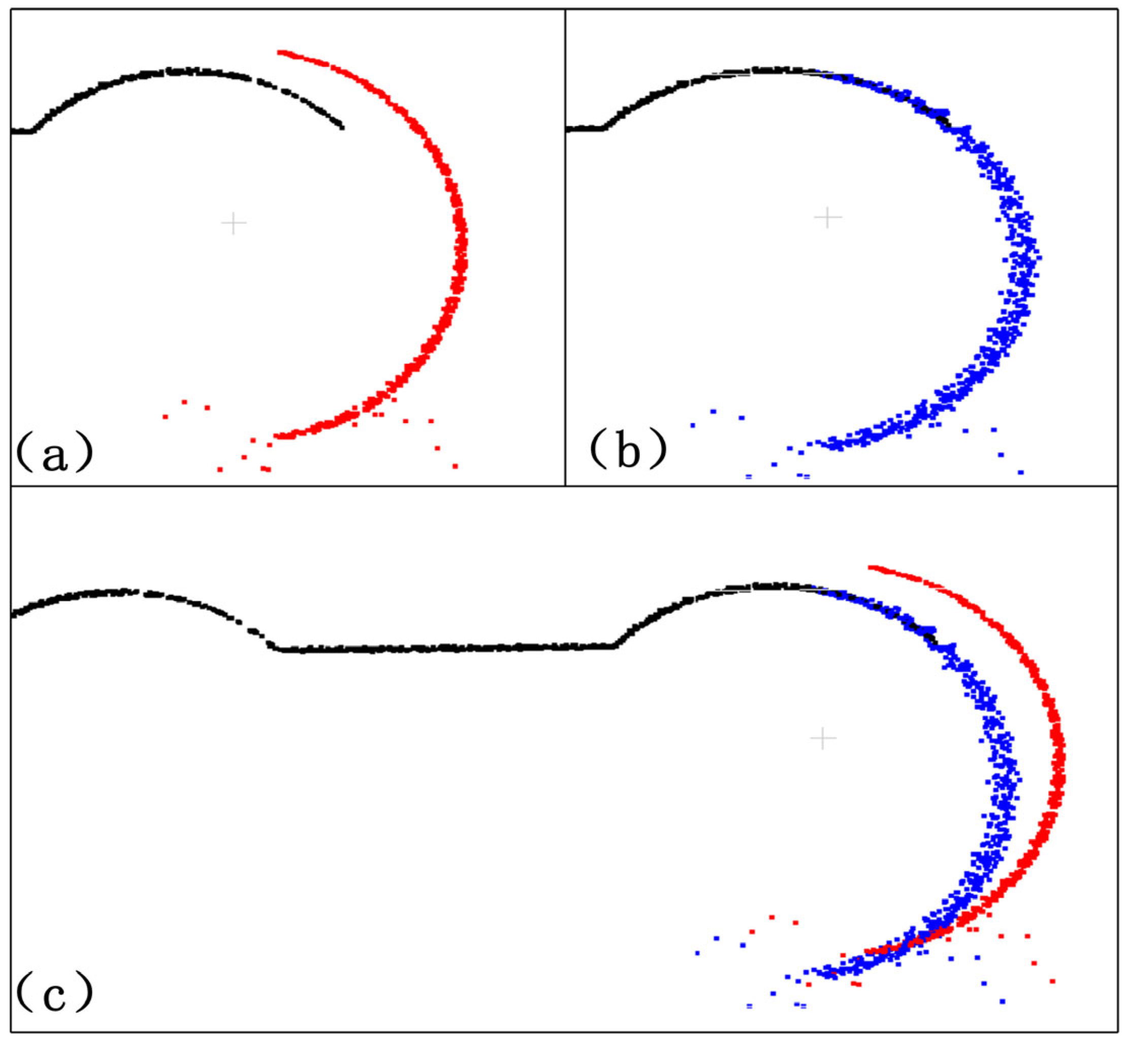
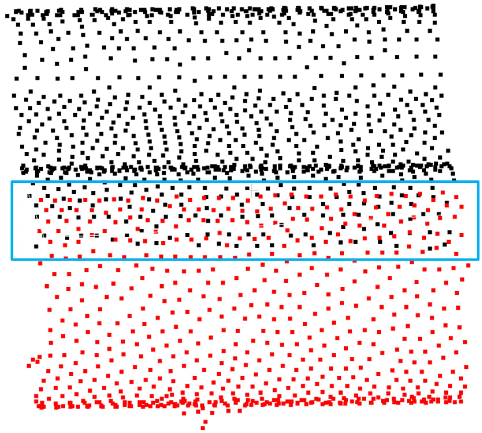
2.3. Coarse Registration

Coarse registration aims to preliminarily align two point clouds by minimizing their spatial separation and maximizing pose overlap. Conventional coarse registration methods typically rely on manual or algorithmic extraction of feature point pairs (e.g., Fast Point Feature Histograms (FPFHs), Intrinsic Shape Signatures (ISSs)) to compute optimal transformation matrices through correspondence matching. FPFHs improve upon Point Feature Histograms (PFHs) by enhancing computational efficiency while preserving local geometric descriptors. PFHs construct feature descriptors through neighborhood geometric relationships at higher computational cost, whereas FPFH achieves faster computation with comparable descriptive capability through algorithmic simplification [23]. ISS automatically detects geometrically salient points in point clouds. These key points capture essential shape characteristics for registration, segmentation, and recognition tasks, exhibiting intrinsic geometric invariance independent of external coordinate systems or scales [24].

While effective for feature-rich point clouds, these methods exhibit significant accuracy degradation under sparse feature conditions. The target structure in this study—a cylindrical arch rib segment with a curved axis line—exhibits smooth surfaces with minimal local features but distinct global geometric regularity. Specifically, localized point clouds from multiple stations inherently conform to a theoretical circular profile (Figure 5), which serves as a geometric constraint to guide position alignment with enhanced rigor.

2.3.1. Initial Pose Estimation

Pose refers to the position and orientation of a point cloud in 3D space [25]. While traditional initial pose estimation aims to provide registration algorithms with a reasonable initial value to reduce computational cost and iterations, thereby improving efficiency and accuracy, this study calculates the initial pose specifically to determine the spatial relationship between the target point cloud (scanned from above) and the source point cloud (scanned externally).

The implementation begins by applying CSF to non-structural data to extract ground point clouds. These ground points are then fitted into a plane using the least-squares method (Figure 6a). Within a defined spatial region, ground point clouds from multiple stations should exhibit high consistency; consequently, their fitted planes share identical geometric parameters (Figure 6b). Given the relative positioning between bridge components and the ground, this invariant plane serves as a reference for partially determining the spatial relationships of different datasets.

Only after establishing these relative positions can the precise localization of both point clouds be achieved:

• The target point cloud is constrained to lie on the theoretical circular arc (the ideal cross-section of the arch rib segment).
• The source point cloud is aligned with the cylindrical surface defined by the segment’s geometry.

This geometric constraint-driven alignment process is illustrated in Figure 6c.

In this section, the initial pose estimation relies on ground plane fitting, with its core assumption being that “ground point clouds can be approximated by an ideal plane.” However, in practical scenarios, there may exist uneven ground surfaces, local occlusions, or multi-source structural interferences (such as ground cables and sundry stacking), which can cause deviations in the traditional least-squares-based plane fitting method. To validate the reliability of the method proposed in this paper under non-ideal conditions, verification was conducted through multiple real-world scenes, as shown in Figure 7a–c. These figures illustrate that after classifying ground points and non-ground points, the ground points are used to fit a plane, which is taken to represent the ground. The fitting results are shown in Figure 7d–f. It can be seen from the elevation distribution histograms (Figure 7g–i) that the plane fitted by this method is less affected by non-ground points, basically coinciding with the ground points, and has strong robustness, so this plane can be regarded as the ground.

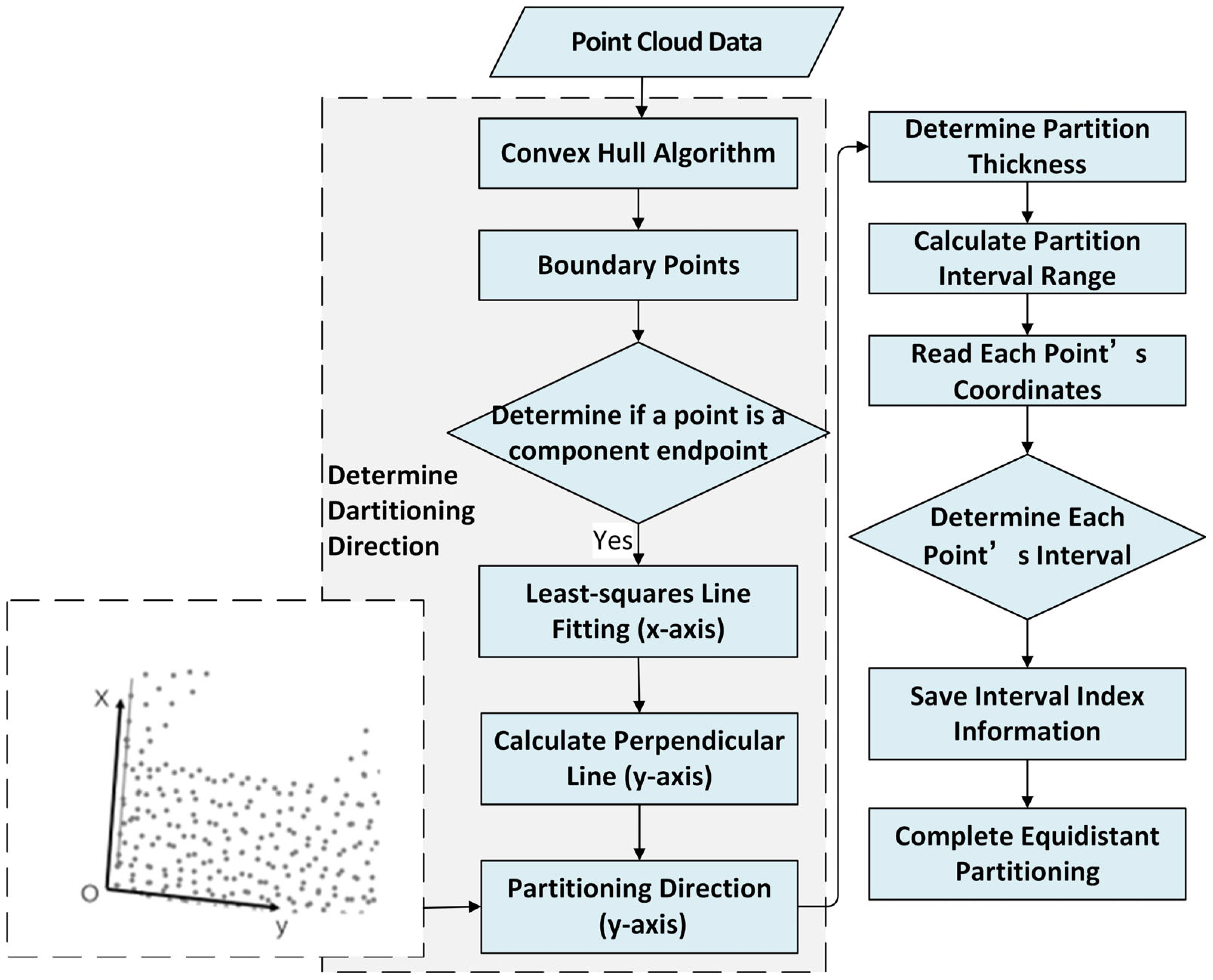
2.3.2. Equidistant Partitioning

This study implements equidistant partitioning on both target and source point clouds using identical intervals, generating multiple groups of corresponding sub-clouds. The partitioning methodology is illustrated in Figure 8. The process initiates with convex hull computation to extract boundary points from raw point clouds.

The Gift Wrapping Algorithm constructs the convex hull by performing the following:

• Selecting the leftmost point as the initial vertex;
• Iteratively identifying adjacent points with minimal angular deviation in a counterclockwise direction;
• Terminating when the search loop returns to the starting point.

Boundary points are filtered to identify segment endpoints, from which the baseline L is fitted [26]. The optimal partitioning direction is determined as the orientation orthogonal to L (denoted as L′). Partition thickness is empirically optimized through iterative trials, with 100 mm identified as the optimal value balancing computational efficiency and registration accuracy. Each point is assigned to a partition interval based on its spatial coordinates relative to the partitioning direction (L′) and thickness. Indexing and classification complete the equidistant partitioning. Figure 9 demonstrates the partitioning results, where color-coding distinguishes individual intervals. For clarity in subsequent discussions, the following applies:

• Target point clouds are abbreviated as upper clouds.
• Source point clouds are termed lateral clouds.

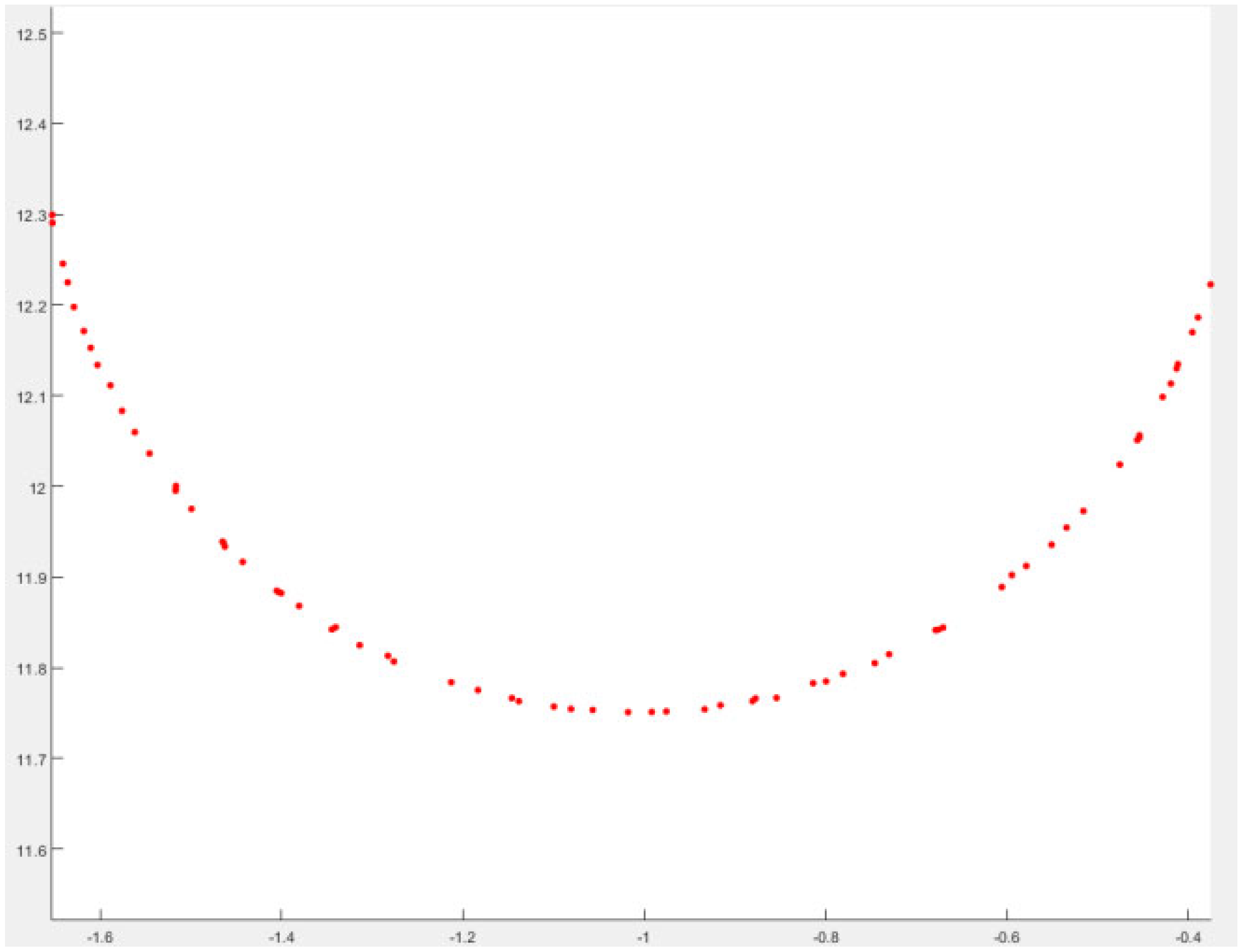
2.3.3. Optimal Projection Plane Calculation

The optimal projection plane is calculated for each partitioned sub-cloud to enable dimensionality reduction, thereby preparing data for subsequent circular fitting. Defined as the 2D plane that optimally projects 3D point clouds into simplified yet geometrically representative distributions, the optimal projection plane transforms complex spatial patterns into analyzable planar configurations.

For this study, the optimal projection plane is specifically defined as the planar surface onto which both upper and lateral sub-clouds project to form a regular circle [27]. Assuming each sub-cloud lies on a cylindrical surface, the task reduces to identifying the cylindrical base plane (i.e., the projection plane). The cylindrical axis direction is determined via vector analysis of three surface points $P_1\left(x_1,y_1,z_2\right), P_2\left(x_2,y_2{,z}_2\right)$, and $P_3(x_3,y_3,z_3)$. Vectors $\overrightarrow{P_1{P}_2}$ and $\overrightarrow{P_1{P}_3}$ are computed, whose cross product yields the normal vector $\overrightarrow{n}$ to the local plane. By statistically analyzing multiple such normals, the global cylindrical axis direction vector $\overrightarrow{v}$ is determined. The projection plane is defined as the surface orthogonal to $\overrightarrow{v}$, corresponding to the cylindrical base.

Projection onto the plane follows the equation $Ax+By+Cz+D=0$, where ${|A,B,C|}^T$ is the unit normal vector of the plane, and $D$ denotes its positional offset from the origin. The orthogonal projection coordinates $(xp,yp,zp)$ are derived by projecting original points along the normal vector direction, as formalized in Equations (1)–(3) and visually illustrated in Figure 10:

$$xp=x\times \left(B^2+C^2\right)-A\times \left(y\times B+z\times C+D\right)/|A,B,C|$$

(1)

$$yp=y\times \left(A^2+C^2\right)-B\times \left(x\times A+z\times C+D\right)/|A,B,C|$$

(2)

$$zp=z\times \left(A^2+B^2\right)-C\times \left(x\times A+y\times B+D\right)/|A,B,C|$$

(3)

2.3.4. Circle Fitting for Projected Data

Each sub-cloud theoretically forms a single circle; thus, both upper and lateral clouds within a group are fitted to circles of equal radii. After projection, only the x and y coordinates are considered for circle fitting. Assuming a circle with center $(x_0,y_0)$ and radius $r$, the equation $(x-x_0)2+(y-y_0)2=r2$ is solved using the least-squares method. For n points $(x_{\mathrm{i}},y_{\mathrm{i}})$, the error function is defined as Equation (4):

$$E={{\sum }_{i=1}^n[{\left(xi-x0\right)}^2+{\left(yi-y0\right)}^2-r^2]}^2$$

(4)

Partial derivatives of $E$ with respect to $x0$, $y0$, and $r$ are computed and set to 0, yielding the system of Equations (5)–(7):

$${\displaystyle \frac{\partial E}{\partial X0}}=4{\sum }_{i=1}^n\left(xi-x0\right)[{\left(xi-x0\right)}^2+{\left(yi-y0\right)}^2-r^2]=0$$

(5)

$${\displaystyle \frac{\partial E}{\partial y0}}=4{\sum }_{i=1}^n\left(yi-y0\right)[{\left(xi-x0\right)}^2+{\left(yi-y0\right)}^2-r^2]=0$$

(6)

$${\displaystyle \frac{\partial E}{\partial r}}=-4{\sum }_{i=1}^n[{\left(xi-x0\right)}^2+{\left(yi-y0\right)}^2-r^2]=0$$

(7)

Solving the system of equations yields the values of $x0$, $y0$, and $r$. Since Equations (5)–(7) are nonlinear, a Newton-Raphson method is employed for numerical solution, with the following steps:

A.

Initial Value Setting: The centroid $(\overline{x},\overline{y})$ of the point cloud, calculated via PCA, is used as the initial center $(x_0^0,y_0^0)$, and the initial radius $r^0$ is set to the average distance from all points to the centroid as Equation (8)

$$r^0={\displaystyle \frac{1}{n}}{\sum }_{i=1}^n\sqrt{{(x_{\mathrm{i}}-\overline{x})}^2+{(y_{\mathrm{i}}-\overline{y})}^2}$$

(8)

B.

Iterative Optimization: In the $k$-th iteration, define the residual function

$$e_i={(x_{\mathrm{i}}-x_0)}^2+{(y_{\mathrm{i}}-y_0)}^2-r^2$$

(9)

and then the error function

$$E={\sum }_{i=1}^n{e}_i^2$$

(10)

Construct the Jacobian matrix $J_K(n\times 3)$ as Equation (11) and the Hessian matrix $H_k(3\times 3)$ as Equation (12):

$$J_{k=i,j}={\displaystyle \frac{\partial e_i}{\partial {\theta }_i}},\theta =[x0,y0,r]$$

(11)

$$H_k\approx J_K^T{J}_K+diag\left({\lambda }_k\right)$$

(12)

where ${\lambda }_k$ is the Levenberg–Marquardt damping factor to improve algorithm stability. Solve the linear system

$$H_k∆{\theta }_k=-J_K^T{e}_k$$

(13)

to obtain the parameter update

$$∆{\theta }_k={[∆x_0,∆y_0,∆r]}^T$$

(14)

and then update the parameters as follows:

$${\theta }_{k+1}={\theta }_k+∆{\theta }_k$$

(15)

C.

Termination Criterion: The iteration terminates when the norm of the parameter update $\parallel \Delta \theta k\parallel <{10}^{-6}$ or the number of iterations exceeds 100.

This approach iteratively converges to the optimal solution and is more suitable for nonlinear least squares problems than linear methods like Singular Value Decomposition, effectively handling the strong nonlinearity in circle fitting.

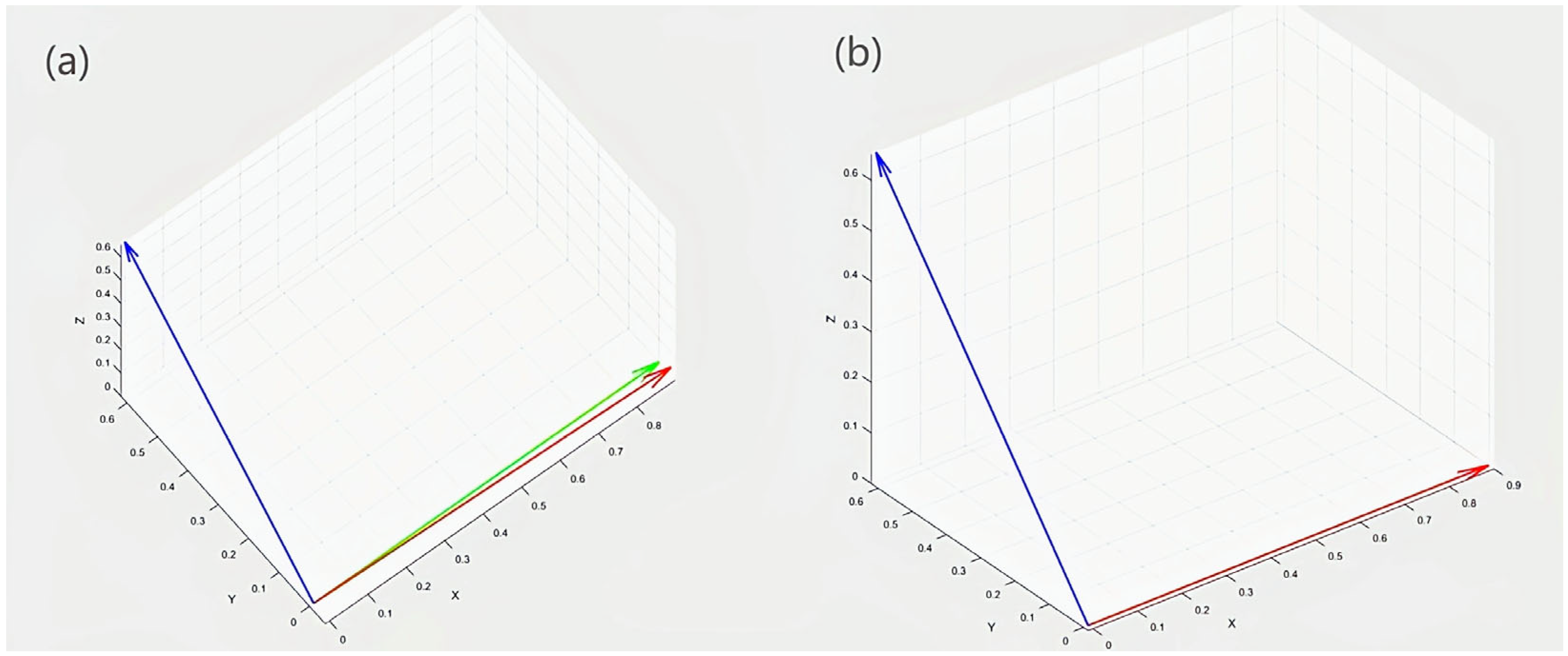
2.3.5. Rigid Transformation (Rotation and Translation)

The investigated registration scenario falls within rigid registration domain. Rigid registration restricts transformations to rotation $\mathit{R}$ and translation $\mathit{t}$, preserving geometric consistency through Equation (16):

$$P’=R·P+t$$

(16)

where $\mathit{P}$ denotes source point cloud coordinates.

In contrast, non-rigid registration permits elastic deformations for objects requiring shape variation accommodation, formulated as Equation (17):

$$T\left(x\right)=R\left(x\right)+D\left(x\right)$$

(17)

where $\mathit{D}\left(\mathit{x}\right)$ represents displacement fields. Methods like Thin-Plate Splines enforce smooth deformation constraints via energy minimization. The adopted rigid approach aligns with CFST arch ribs’ mechanical behavior during fabrication, where elastic deformation remains negligible.

A.

Rotation Parameter Calculation

The rotation parameters of point clouds consist of two components: the rotation angle and the rotation axis. First, the rotation angle is determined by computing the directional vectors $\overrightarrow{v1}(x1,y1,z1)$ and $\overrightarrow{v2}(x2,y2,z2)$ for upper and lateral circles in each sub-cloud using the cylindrical axis calculation method described earlier. The rotation angle $\theta$ is then derived through the vector dot product Formula (18) and vector magnitude Formula (19), as expressed in Equation (21). Second, the rotation axis is obtained via the cross-product Formula (20) of the two directional vectors, yielding the rotation axis direction vector $\overrightarrow{n}=(xn,yn,zn)$.

$$\overrightarrow{v1}\times \overrightarrow{v2}=|\overrightarrow{v1}||\overrightarrow{v2}|cos\theta$$

(18)

$$|\overrightarrow{v1}|=\sqrt{{x1}^2+{y1}^2+{z1}^2}, |\overrightarrow{v2}|=\sqrt{{x2}^2+{y2}^2+{z2}^2}$$

(19)

$$\theta =\mathrm{a}\mathrm{r}\mathrm{c}\mathrm{c}\mathrm{o}\mathrm{s}\left({\displaystyle \frac{\overrightarrow{v1}\times \overrightarrow{v2}}{|\overrightarrow{v1}||\overrightarrow{v2}|}}\right)$$

(20)

$$\overrightarrow{n}=\overrightarrow{v1}\times \overrightarrow{v2}$$

(21)

B.

Applying Rotation Parameters

Given the rotation axis direction vector n and rotation angle $\theta$, a rotation matrix $R$ is constructed using Rodrigues’ rotation formula [28] (RF) to perform axis-angle rotation in 3D space. Let $\overrightarrow{n}$ be a unit vector ($|\overrightarrow{n}|=1$). The Rodrigues formula defines the rotation matrix as Equation (22):

$$R=I+sin\theta K+\left(1-cos\theta \right)K^2$$

(22)

where $I$ is the identity matrix. $K$ is the skew-symmetric matrix associated with n, defined by Equation (23):

$$K=\left(\begin{array}{ccc}0& -zn& yn\\ zn& 0& -xn\\ -yn& -xn& 0\end{array}\right)$$

(23)

Point cloud coordinates $P(x,y,z)$ are converted to homogeneous coordinates $\tilde{P}(x,y,z,1)$. The rotation operation is achieved by matrix multiplication: ${\tilde{P}}^1=R\tilde{P}$, aligning the axes of both clouds (see Figure 11).

C.

Translation Parameter Calculation

After the rotation is completed, calculate the translation vector to make the centers of the two circles coincide. Suppose the centers of the two circles are $O\left(x0,y0,z0\right)$ and $O1(x1,y1,z1)$. The translation vector $\overrightarrow{t}$ is the vector required to move one center to the position of the other center. The specific calculation formula for $\overrightarrow{t}$ is Equation (24):

$$\overrightarrow{t}=O1-O=\left(x1-x0,y1-y0,z1-z0\right)$$

(24)

D.

Applying Translation Parameters

Let $\overrightarrow{t}=\left(tx,ty,tz\right)$, and construct the translation matrix $T$ (Equation (25)):

$$T=\left(\begin{array}{cccc}1& 0& 0& tx\\ 0& 1& 0& ty\\ 0& 0& 1& tz\\ 0& 0& 0& 1\end{array}\right)$$

(25)

Multiply the rotated point cloud ${\tilde{P}}^1$ by the matrix $T$ to obtain the final point cloud after rotation and translation, thus completing the coarse registration of the point cloud.

2.4. Fine Registration

The core principle of our coarse registration lies in leveraging the circular cross-section geometry of tubular joints to align multi-station data. However, enforcing perfect circular fitting for each sub-cloud introduces local optima during registration. These local optima optimize alignment within individual sub-clouds but induce minor deformations in the global structure, preventing optimal overall registration. Notably, the partitioned source point clouds undergo rotation and translation as sub-clouds. Despite local deformations, their transformation parameters remain correlated due to the underlying tubular joints curvature, preserving spatial coherence across the global structure. To address this limitation, we implement fine registration on the coarsely aligned data to refine global consistency.

The ICP algorithm, a classical fine registration method, iteratively optimizes point correspondences to estimate transformation parameters. The ICP algorithm minimizes the distance between two point clouds by solving the transformation between the source point cloud set $Pi=(P1,\dots ,Pa)T$ and the target point cloud set $Qi=(Q1,\dots ,Qb)T$, where a and b represent the number of points in the two sets [29]. By calculating the rotation matrix R and the translation matrix t, the error function $E(R,t)$ is obtained. A smaller value of $E(R,t)$ indicates better accuracy. Essentially, it aims to find the optimal solution $(R,t)$.

For $E(R,t)$, and the formula is as follows (26):

$$E\left(R,t\right)={\displaystyle \frac{1}{n}}{\sum }_{i=1}^n{‖q_i-(R{p}_i+t)‖}^2$$

(26)

In the formula, $q_i$ and $p_i$ represent a point in $Q$ and $P,$ respectively. The specific process of the ICP algorithm is as follows:

A.

Randomly select a point $p_i$ from the source point set $P$.

B.

Find the corresponding point $q_i$ in the target point set $Q$ such that $‖q_i-p_i‖=min$.

C.

Calculate R and t to minimize $E(R,t)$. Compute cross-covariance matrix H.

$$H={\sum }_{i=1}^n\left(p_i-\mu p\right){(q_i-\mu Q)}^T$$

(27)

where $\mu p={\displaystyle \frac{1}{n}}\sum p_i$ and $\mu Q={\displaystyle \frac{1}{n}}\sum q_i$ are centroid coordinates. Perform singular value decomposition using Formula (28):

$$H=U\sum V^T$$

(28)

The optimal rotation and translation are then given by Formula (29):

$$R=V{U}^T,t=\mu Q-R\mu p$$

(29)

D.

Transform $p_i$ using $R$ and $t$ obtained in step C to obtain a new point set: $p_i^{’}=R{p}_i+t,p_i\in P$, where $p_i$ in $P$.

E.

Calculate the average distance between $p_i$ and its corresponding point $q_i$ in the point set $Q$ using Formula (30):

$$d={\displaystyle \frac{1}{n}}{\sum }_{i=1}^n{‖p_i^{’}-q_i‖}^2$$

(30)

F.

Set a threshold. Stop the iteration when $d$ is less than the threshold; otherwise, return to step B until the condition is met.

However, ICP exhibits significant errors under ambiguous correspondences—a drawback amplified by deformations from coarse registration. The CPD algorithm [30] frames registration as a probability density estimation problem. It models the source point cloud as a transformed (rotated, translated, or deformed) and noise-corrupted version of the target. A Gaussian Mixture Model (GMM) represents the source points as probability density peaks within the target distribution. Registration is achieved by maximizing the likelihood of source points under this GMM, thereby solving for optimal rigid/non-rigid transformations.

Let the source points $Mi=(M1,\dots ,Mn)T$ form GMM centroids, and target points $Ti=(T1,\dots ,Tm)T$ serve as observed data [31], where $n$ and $m$ denote the number of points in the source and target sets, respectively. The GMM probability density is given by Equations (31) and (32):

$$p\left(t\right)=\omega {\displaystyle \frac{1}{j}}+(1-\omega ){\sum }_{x=1}^i{\displaystyle \frac{1}{i}}p(t\left|x\right.)$$

(31)

$$p\left(t\left|x\right.\right)={\displaystyle \frac{1}{{\left(2\pi {\sigma }^2\right)}^{\frac{3}{2}}}}\exp (-{\displaystyle \frac{{‖t-Mi‖}^2}{2{\sigma }^2}})$$

(32)

Here, $p\left(t\left|x\right.\right)$ is the GMM basis function, $t$ is the translation variable, $\omega \in \left[\mathrm{0,1}\right]$ weights outlier points, and $\sigma$ is estimated via minimizing the negative log-likelihood:

$$E\left(\theta ,{\sigma }^2\right)=-{\sum }_{n=1}^N\log {\sum }_{m=1}^{M}p\left(x\right)p\left(t\left|x\right.\right)$$

(33)

Gradient descent on Equation (33) yields update rules (34) and (35). Iterations terminate upon convergence, solving for transformation parameters.

$$Q\left(W\right)={\sum }_{m=1}^M{\sum }_{n=1}^{N}p\left(m\left|x_n\right.\right){‖{\displaystyle \frac{x_n-y_m-G(m,R)W}{c}}‖}^2/2^{c^2}$$

(34)

$$P_{mn}=\exp (-{\displaystyle \frac{1}{2}}{‖{\displaystyle \frac{y_m-x_n}{c}}‖}^2)/{\sum }_{m=1}^M\exp (-{\displaystyle \frac{1}{2}}{‖{\displaystyle \frac{y_m-x_n}{c}}‖}^2)$$

(35)

From a correspondence perspective, the CPD algorithm fundamentally establishes global correspondences between source and target point clouds. Diverging from rigid one-to-one correspondence determination, it employs probabilistic distribution modeling to associate each source point with multiple target points. This approach enables flexible point matching while preserving spatial coherence—defined as the consistency of neighboring points’ spatial relationships. The key advantage lies in its emphasis on global coherence over local pairwise matches, effectively addressing registration scenarios with local deformations induced by coarse alignment.

In practice, as a binary tree structure, k-d trees recursively partition the point cloud space into subregions using hyperplanes perpendicular to coordinate axes, progressively dividing k-dimensional data (such as 3D point cloud coordinates) into leaf nodes. This process allows the CPD algorithm to quickly locate nearest neighbors in the target point cloud during probability density matching, reducing the time complexity of traditional point-wise search. To enhance computational efficiency for large-scale point clouds, this study employs k-d trees to construct spatial indexing, accelerating the nearest-neighbor search in CPD’s probability density matching process. The coarsely registered point cloud is designated as the target dataset. The CPD algorithm is then applied to align the source cloud with this target, iteratively refining the coarse registration outcome.

3. Experimental Analysis and Discussion

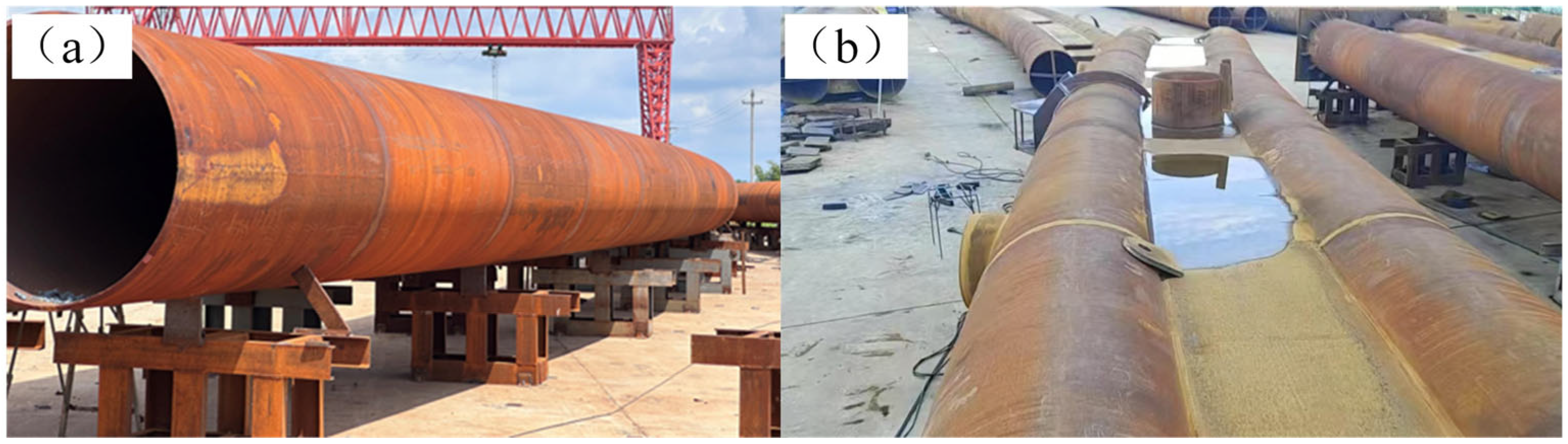
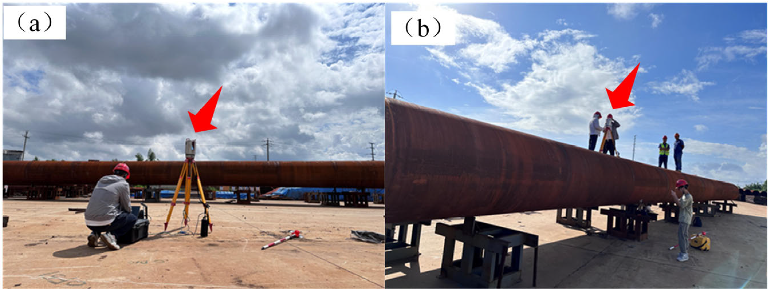
3.1. Experimental Data

This study is conducted on an in situ CFST arch bridge project in Qinzhou, Guangxi Zhuang Autonomous Region. The bridge features a 95 m half-through arch span designed for urban-A grade loads. The main arch rib adopts a dumbbell-shaped CFST cross-section, comprising twin steel tubes (diameter = 1.26 m, wall thickness = 26–28 mm) filled with C50 self-compacting concrete. The investigation focuses on the prefabricated L3 arch segment located at the arch springing, measuring approximately 2.2 m in length, whose on-site structural form is illustrated in Figure 12.

Experimental data acquisition employed a Riegl VZ-1000 terrestrial laser scanner (manufactured by RIEGL Laser Measurement Systems GmbH, Horn, Austria) during thermally stable nighttime periods (28 ± 0.5 °C). Scanning stations were strategically positioned on the upper and lateral surfaces of the target segment (Figure 13). Aiming at the point cloud registration problem caused by the segmented point clouds scanned at multiple stations, this study proposes a coarse registration method that uses the local geometric characteristics of the segmented point clouds for constraint and uses the CPD algorithm to improve registration accuracy, providing technical support for the digital acceptance of bridge prefabricated components.

3.2. Coarse Registration Accuracy

Prior to applying the proposed coarse registration method, the segment point clouds exhibited significant stratification in overlapping regions, as illustrated in Figure 14a. Here, the preprocessed upper scan (black point cloud) and lateral scan (red point cloud) display pronounced spatial misalignment. Following coarse registration (Figure 14b), the realigned lateral scan (blue point cloud) shows remarkable congruence with the upper scan (black point cloud), completely eliminating stratification within the overlapping zone.

Analysis of post-registration local details (Figure 15) reveals consistent circular distributions at five sampled positions (Figure 15a–e). Crucially, no stratification is observed at any position, demonstrating the efficacy of the coarse registration method in achieving the intended alignment.

3.3. Fine Registration Performance Evaluation

RMSE serves as a quantitative metric for registration accuracy in point cloud alignment, defined as Equation (36):

$$RMSE=\sqrt{{\displaystyle \frac{\sum _i^N{‖T{P}_i-q_i‖}^2}{N}}}$$

(36)

Given the low-overlap characteristics of the test point clouds, calculating RMSE across entire datasets would misrepresent true alignment accuracy. Thus, evaluation is restricted to overlapping regions (Figure 16). As summarized in

Table 1. Overlap region registration error table unit: m.

Method	RMSE	Improvement	Time
Coarse registration	0.031	-	-
NDT	0.028	9.7%	8.13 s
ICP	0.018	41.9%	12.22 s
CPD	0.004	87.0%	20.21 s
CPD (kd-tree)	0.004	87.0%	13.30 s

, coarse registration achieves an RMSE of 0.031 m, while conventional CPD fine registration methods yield 0.028 m (Normal Distribution Transform (NDT)) and 0.018 m (ICP). The proposed KD-tree-accelerated CPD fine registration further reduces it to 0.004 m—demonstrating 77.8% and 85.7% precision improvements over ICP and NDT, respectively, with an overall 87% enhancement compared to coarse registration. Notably, this method accomplishes the same precision in 13.30 s, a 34.2% reduction from the 20.21 s required by conventional CPD.

To clearly demonstrate the registration accuracy between the registered target point cloud and the source point cloud, this paper also employs the coefficient of determination $R$-Square ($R2$), with its detailed calculation provided in Equation (37)

$$R^2={\displaystyle \frac{\sum _{i=1}^n{\left({p_i}^{’}-q_i\right)}^2}{\sum _{i=1}^n{\left(p_i-q_i\right)}^2}}$$

(37)

Coarse registration achieves $R2$ = 0.889, indicating that 88.9% of the initial misalignment between source and target clouds is eliminated. Conventional fine registration methods yield $R^2$ = 0.903 (NDT) and 0.957 (ICP), corresponding to residual discrepancies of 9.7% and 4.3%, respectively. The proposed CPD fine registration elevates $R2$ to 0.995—demonstrating 3.9% and 10.2% improvements over ICP and NDT, with merely 0.5% residual discrepancy, which confirms the superior congruence achieved by the CPD framework.

A quantitative analysis of spatial distances between corresponding points in overlapping regions (as depicted in Figure 17a) reveals the following: Coarse registration achieves sub-centimeter accuracy (≤0.004 m) for 16% of points, while 84% of points exhibit errors exceeding 0.01 m. Further quantification of refined registration accuracy demonstrates distinct algorithmic performances: For NDT fine registration (Figure 17b), the error distribution shows minimal improvement compared to coarse registration, with over 80% of points still exceeding 0.01 m accuracy. ICP fine registration (Figure 17c) significantly reduces high-error points, stabilizing 92% of correspondences around 0.005 m and eliminating errors above 0.01 m. CPD fine registration (Figure 17d) demonstrates superior performance, with 95% of points converging to approximately 0.004 m and a maximum observed error of 0.006 m. This evidences that CPD fine registration achieves a substantial enhancement in registration precision compared to both coarse registration and other fine registration methods.

4. Conclusions

This study proposes a coarse-to-fine registration framework for multi-station point cloud alignment of bridge components using local geometric features. Precision analysis in overlapping regions yields three key findings:

A.

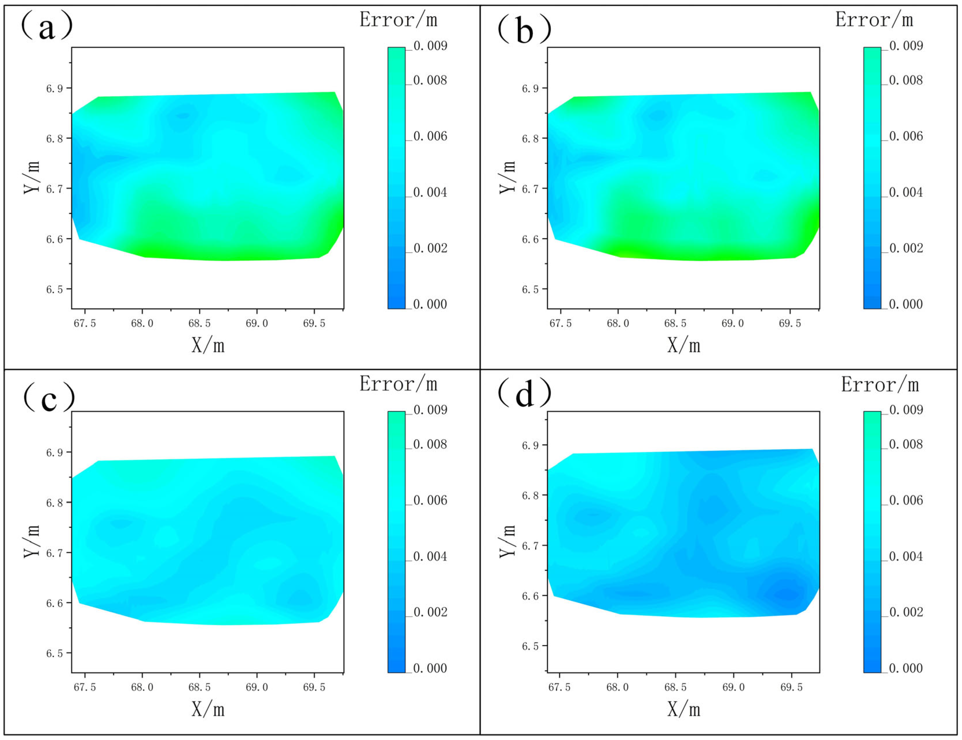
Coarse Registration Performance: The initial alignment achieves RMSE = 0.031 m with R² = 0.889, eliminating 88.9% of initial misalignment. Error distribution analysis reveals only 16% of corresponding points reach sub-centimeter accuracy (≤0.004 m), while 84% exhibit registration errors exceeding 0.01 m (Figure 17a).

B.

Fine Registration Comparison: Conventional fine registration methods show differentiated performance—NDT reduces RMSE to 0.028 m (9.7% improvement) with R² = 0.903, while ICP achieves RMSE = 0.018 m (41.9% improvement) and R² = 0.957. The proposed KD-tree-accelerated CPD method demonstrates superior precision with RMSE = 0.004 m (87% improvement) and R² = 0.995, leaving merely 0.5% residual error. This represents 3.9% and 10.2% R² enhancements over ICP and NDT, respectively (Table 1).

C.

Error Distribution Characteristics: Post-NDT refinement maintains >80% points with >0.01 m errors (Figure 17b), whereas ICP stabilizes 92% correspondences around 0.005 m (Figure 17c). The CPD algorithm exhibits optimal performance with 95% points converging to 0.004 m and maximum observed error <0.006 m (Figure 17d). Remarkably, it completes computation within 13.30 s, achieving 34.2% acceleration over conventional CPD, confirming its engineering practicality.

While advancing point cloud registration for CFST arch rib segments, both methods exhibit substantial optimization potential:

A.

Theoretical Extension: Generalize the local geometric constraint-based registration theory to broader engineering scenarios (e.g., irregular steel trusses, composite decks).

B.

Algorithm Enhancement: Develop adaptive CPD variants incorporating deformation priors for complex structural geometries.

C.

Investigation into the Mechanism of Point Cloud Density on Registration Accuracy: The current study does not systematically analyze the quantitative impact of point cloud density distribution (such as edge sparse areas and far-field low-density areas) on registration accuracy. In the future, multi-density downsampling experiments will be conducted, combined with error heatmap visualization techniques, to analyze the error propagation laws in sparse regions.

The novel point cloud registration paradigm proposed in this study establishes a technical foundation for intelligent infrastructure lifecycle management, demonstrating significant potential in disaster risk early-warning applications [32].

References

1. Chen, J.G.; Wei, J.; Zhou, J.P.; Liu, J. Application of concrete-filled steel tube arch bridges in China: Current status and prospects. China Civ. Eng. J. 2017, 50, 50–61. [Google Scholar]
2. Song, Y. Research on Application Maturity of Three—Dimensional Laser Scanning Technology in Building Construction Stage. Master’s Thesis, China University of Mining and Technology, Xuzhou, China, 2022. [Google Scholar]
3. Gao, Y. Application Research of 3D Laser Scanning Technology in Slope Monitoring. Master’s Thesis, Chongqing Jiaotong University, Chongqing, China, 2021. [Google Scholar] [CrossRef]
4. Luo, B.; Wang, J.; Luo, L.; Guo, Y. Application of backpack 3D laser scanning in urban large scale topographic map survey. Bull. Surv. Mapp. 2024, 187–190+196. [Google Scholar] [CrossRef]
5. Arseni, M.; Roman, O.; Cucoara, C.; Georgescu, L.P. Application of Mobile Mapping System for a Modern Topography. J. Appl. Eng. Sci. 2024, 14, 186–193. [Google Scholar] [CrossRef]
6. Jia, S.; de Vugt, L.; Mayr, A.; Liu, C.; Rutzinger, M. Location and orientation united graph comparison for topographic point cloud change estimation. ISPRS J. Photogramm. Remote Sens. 2025, 219, 52–70. [Google Scholar] [CrossRef]
7. Chen, Y.; Wu, T.; Chen, Z. Error Analysis and Control Based on 3D Laser Scanning Measurement for Large-scale Bridge. Railw. Eng. 2022, 62, 96–100. [Google Scholar]
8. Wang, Q.A.; Zhang, C.; Ma, Z.G.; Ni, Y.Q. Modelling and forecasting of SHM strain measurement for a large-scale suspension bridge during typhoon events using variational heteroscedastic Gaussian process. Eng. Struct. 2022, 251, 113554. [Google Scholar] [CrossRef]
9. Wang, Q.A.; Dai, Y.; Ma, Z.G.; Wang, J.F.; Lin, J.F.; Ni, Y.Q.; Ren, W.X.; Jiang, J.; Yang, X.; Yan, J.R. Towards high-precision data modeling of SHM measurements using an improved sparse Bayesian learning scheme with strong generalization ability. Struct. Health Monit. 2024, 23, 588–604. [Google Scholar] [CrossRef]
10. Behfar, G.; Georgios, B.; Susan, T. Restoration Curves for Infrastructure: Preliminary Case Study on a Bridge in Quebec. Inst. Civ. Eng.-Bridge Eng. 2021, 175, 1–17. [Google Scholar]
11. Chang, S. Research on Digital Pre-Assembly Technology of Tubes Based on 3D Laser Scanning Technology. Master’s Thesis, Beijing University of Civil Engineering and Architecture, Beijing, China, 2021. [Google Scholar] [CrossRef]
12. Xu, A.; Rao, L.; Fan, G.; Chen, N. Fast and high accuracy 3D point cloud registration for automatic reconstruction from laser scanning data. IEEE Access 2023, 11, 42497–42509. [Google Scholar] [CrossRef]
13. Leitenstern, M.; Alten, M.; Bolea-Schaser, C.; Kulmer, D.; Weinmann, M.; Lienkamp, M. FlexCloud: Direct, Modular Georeferencing and Drift-Correction of Point Cloud Maps. arXiv 2025, arXiv:2502.00395. [Google Scholar]
14. Ji, J. Research on Registration Method of 3D Laser Scanner in Factory. Master’s Thesis, North China University of Science and Technology, Tangshan, China, 2019. [Google Scholar]
15. Yang, J.; Sun, H. Edge feature enhancement and hierarchical attention fusion for low-overlap point cloud registration. J. Image Graph. 2024, 29, 3739–3755. [Google Scholar] [CrossRef]
16. Fu, Y.; Chen, P.; Guo, G.; Liu, X. Application of the point cloud registration method based on 4PCS and SICP in rail wear calculation. J. Electron. Meas. Instrum. 2022, 36, 210–218. [Google Scholar] [CrossRef]
17. Sun, W.; Yuan, H.; Liu, N.; Liu, Q.; Shu, S. Fast registration algorithm combining contour features for line laser point clouds. J. Electron. Meas. Instrum. 2021, 35, 156–162. [Google Scholar] [CrossRef]
18. Liu, R.F.; Wang, F.; Ren, H.W.; Wang, M.; Yang, J. Road scene laser point cloud registration method based on geographical object features. Chin. J. Lasers 2022, 49, 1810002. [Google Scholar]
19. ISO 2768-1:1989; General Tolerances—Part 1: Tolerances for Linear and Angular Dimensions Without Individual Tolerance Indications. International Organization for Standardization: Geneva, Switzerland, 1989.
20. Zhang, W.; Qi, J.; Wan, P.; Wang, H.; Xie, D.; Wang, X.; Yan, G. An easy-to-use airborne LiDAR data filtering method based on cloth simulation. Remote Sens. 2016, 8, 501. [Google Scholar] [CrossRef]
21. Walfish, S. A review of statistical outlier methods. Pharm. Technol. 2006, 30, 82. [Google Scholar]
22. Schubert, E.; Sander, J.; Ester, M.; Kriegel, H.P.; Xu, X. DBSCAN revisited, revisited: Why and how you should (still) use DBSCAN. ACM Trans. Database Syst. (TODS) 2017, 42, 1–21. [Google Scholar] [CrossRef]
23. Li, P.; Wang, J.; Zhao, Y.; Wang, Y.; Yao, Y. Improved algorithm for point cloud registration based on fast point feature histograms. J. Appl. Remote Sens. 2016, 10, 045024. [Google Scholar] [CrossRef]
24. Li, Y.; Fei, R.; Zhang, T. An Improved Semi-Dense Iterative Closest Point Registration Algorithm Fusing Intrinsic Shape Signatures and Curvature Feature. In Proceedings of the 2024 International Conference on Intelligent Computing and Robotics (ICICR), Dalian, China, 12–14 April 2024; IEEE: Beijing, China, 2024; pp. 78–82. [Google Scholar]
25. Deng, B.; Yao, Y.; Dyke, R.M.; Zhang, J. A survey of non-rigid 3D registration. Comput. Graph. Forum 2022, 41, 559–589. [Google Scholar] [CrossRef]
26. Keller, W.; Borkowski, A. Thin plate spline interpolation. J. Geod. 2019, 93, 1251–1269. [Google Scholar] [CrossRef]
27. Chen, W.; Liu, J.; Yang, H.; Pang, F.; Zhao, H.; Zhang, R. Aircraft Blade Point Cloud Registration Based on Surface Edge Extraction. Appl. Laser 2024, 44, 196–203. [Google Scholar] [CrossRef]
28. Dai, J.S. Euler–Rodrigues formula variations, quaternion conjugation and intrinsic connections. Mech. Mach. Theory 2015, 92, 144–152. [Google Scholar] [CrossRef]
29. Xu, Z.; Dong, L.; Wu, J. LiDAR point cloud registration with improved ICP algorithm. Bull. Surv. Mapp. 2024, 1–5. [Google Scholar]
30. Myronenko, A.; Song, X. Point set registration: Coherent point drift. IEEE Trans. Pattern Anal. Mach. Intell. 2010, 32, 2262–2275. [Google Scholar] [CrossRef] [PubMed]
31. Liu, Y. CPD Algorithm for Registration Based on Feature Point Detection. Electron. Technol. 2018, 47, 14–16. [Google Scholar]
32. Calò, M.; Ruggieri, S.; Doglioni, A.; Morga, M.; Nettis, A.; Simeone, V.; Uva, G. Probabilistic-based assessment of subsidence phenomena on the existing built heritage by combining MTInSAR data and UAV photogrammetry. Struct. Infrastruct. Eng. 2024, 1–16. [Google Scholar] [CrossRef]
Figure 1. Registration workflow comprises three stages: Point cloud preprocessing, Coarse Registration, Fine Registration.
Buildings 15 02130 g001
Figure 2. A hybrid preprocessing strategy.
Buildings 15 02130 g002
Figure 3. Component classification schematic.
Buildings 15 02130 g003
Figure 4. Processed single-segment data.
Buildings 15 02130 g004
Figure 5. Coarse registration flowchart.
Buildings 15 02130 g005
Figure 6. Initial pose determination schematic: (a) ground plane fitting, (b) same plane, and (c) initial pose determination.
Buildings 15 02130 g006
Figure 7. Initial (ac) represent the uneven ground scene, occlusion scene, and multi-structural interference scene, respectively. Red denotes ground point clouds, and blue denotes non-ground point clouds. (df) show the results of plane fitting for ground data, where green represents fitted plane points. (gi) are the elevation distribution histograms for the corresponding scenes.
Buildings 15 02130 g007
Figure 8. Equidistant partitioning flowchart.
Buildings 15 02130 g008
Figure 9. Flowchart equidistant partitions: (a) upper clouds and (b) lateral clouds.
Buildings 15 02130 g009
Figure 10. Projection.
Buildings 15 02130 g010
Figure 11. Direction vector (a) pre rotation and (b) post rotation.
Buildings 15 02130 g011
Figure 12. On-site diagram of the experimental object. (a) Side of the segment (b) Top of the component.
Buildings 15 02130 g012
Figure 13. On-site setup of scanning instruments. (a) Side setup of stations. (b) Top setup of stations.
Buildings 15 02130 g013
Figure 14. Overall comparison before and after registration. (a) represents the state before registration, (b) represents the state after registration, and (c) represents the overall data before and after registration.
Buildings 15 02130 g014
Figure 15. Post-registration local details. (ae) show the point cloud registration at different positions.
Buildings 15 02130 g015
Figure 16. The point cloud overlap region is within the blue dashed line.
Buildings 15 02130 g016
Figure 17. (a) Coarse registration results. (b) NDT fine registration. (c) ICP fine registration. (d) CPD Fine registration results.
Buildings 15 02130 g017