Assessment of Knot-Induced Degradation in Timber Beams: Probabilistic Modeling and Data-Driven Prediction of Load Capacity Loss


 and
and
Abstract
1. Introduction
2. Materials and Methods
2.1. Loading Test and Method
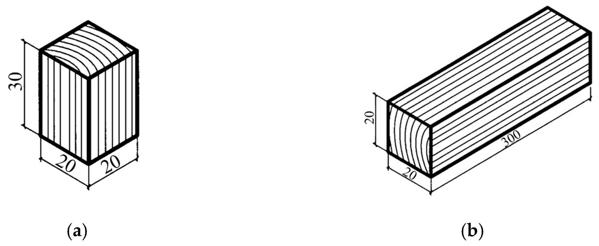
2.1.1. Determination of Material Strength
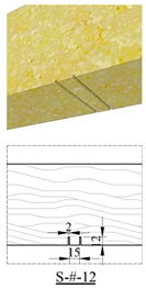
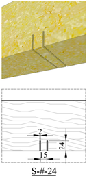
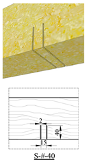
2.1.2. Details of Specimens
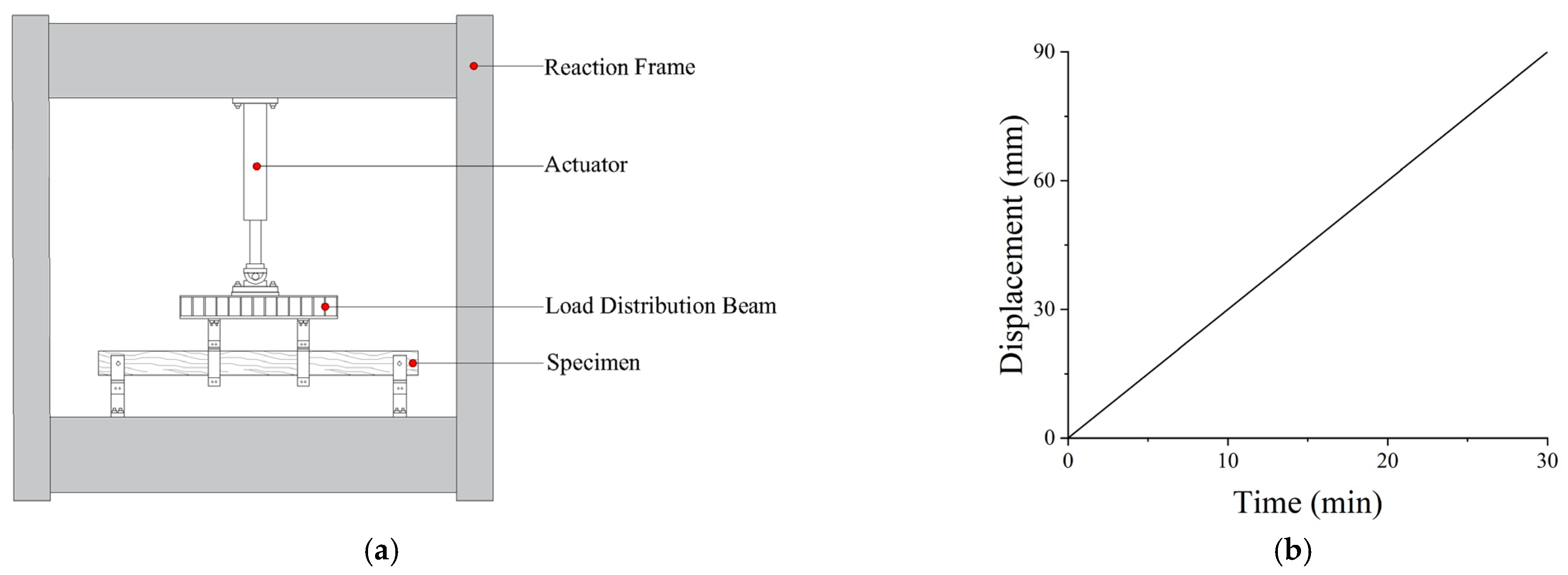
2.1.3. Loading Devices and Loading Protocols
2.2. Monte Carlo Simulation
2.2.1. Bearing Capacity Reduction Function
- Damage: the percentage reduction in the load-carrying capacity of the beam; this value is 0% for defect-free beams.
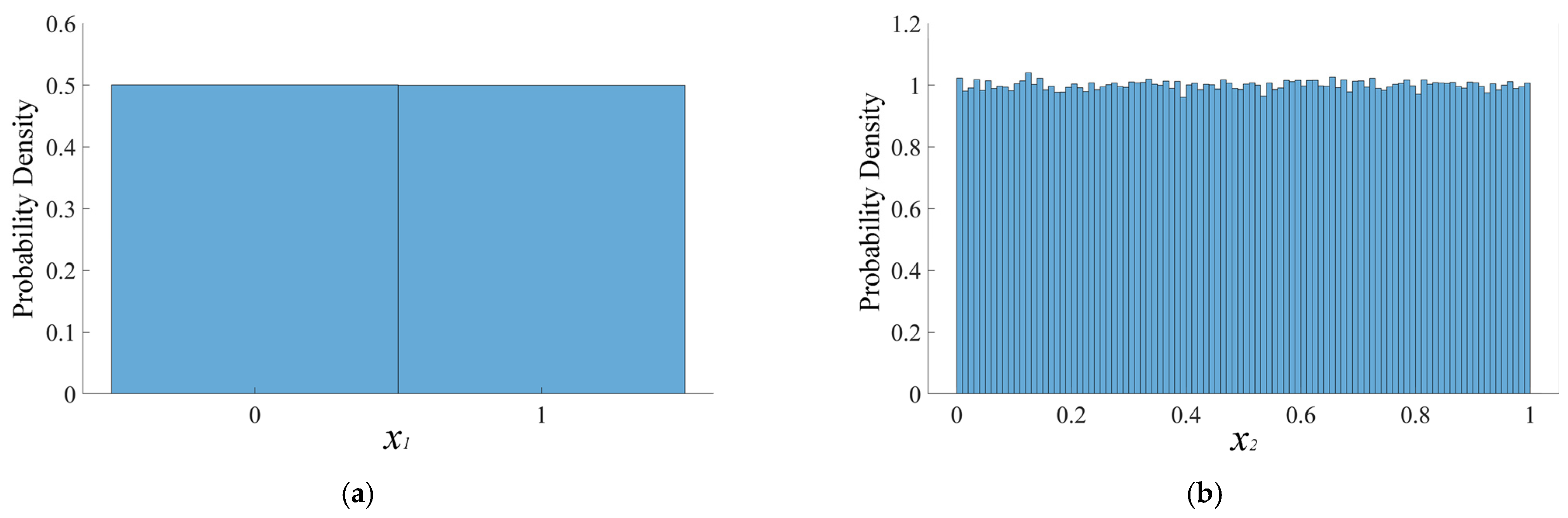
- x1: The positional parameter indicating the location of the timber knot relative to the beam’s cross-section. When the knot is located in the compression (upper) zone, x1 = 0; when located in the tension (lower) zone, x1 = 1.
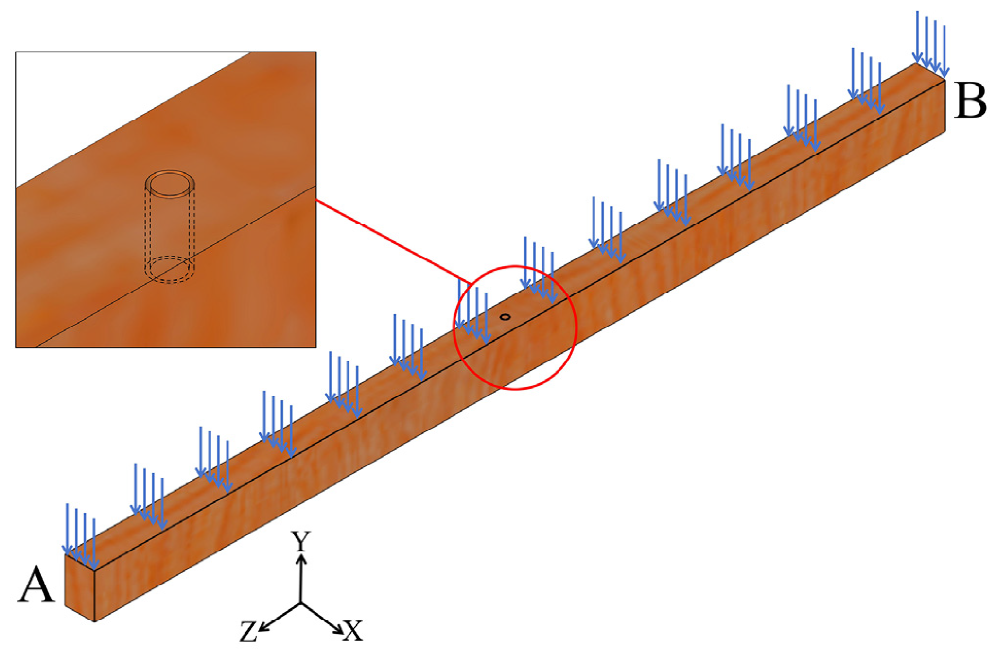
- x2: The normalized longitudinal position of the timber knot along the beam’s length. When the knot is at the end A of the beam, x2 = 0; when at end B, x2 = 1
- x3: the diameter of the timber knot.
- x4: the depth of the timber knot.
2.2.2. Modeling of Stochastic Timber Knots
2.3. MATLAB-Based Machine Learning
2.3.1. Machine Learning Process
- (1)
- Data pre-processing
- (2)
- Model construction
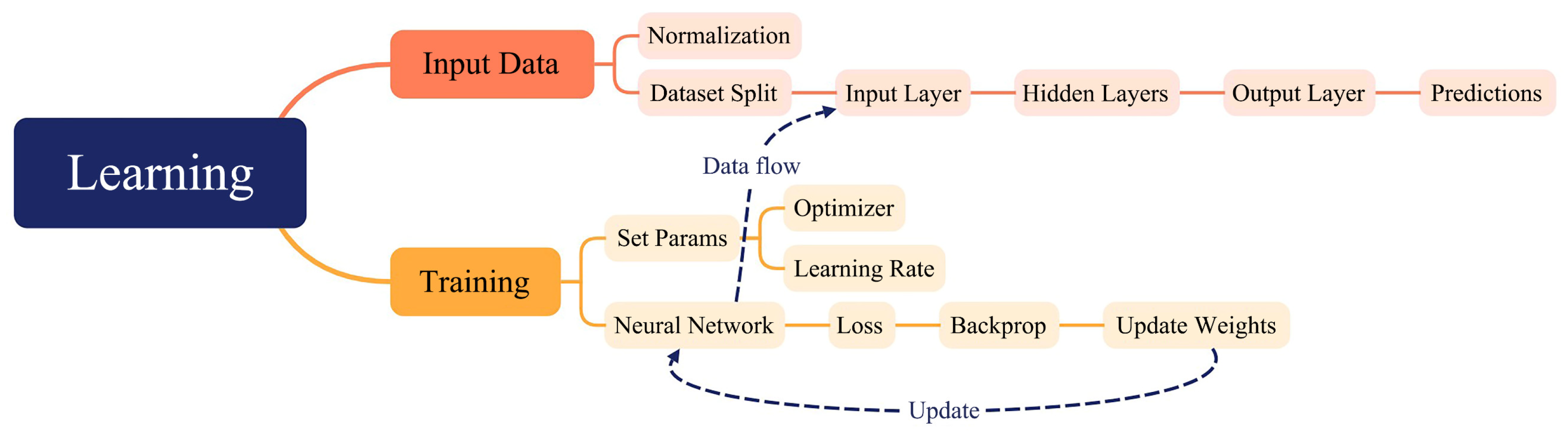
- Input Layer: receives three features: knot position (x2), diameter (x3), and depth (x4).
- Hidden Layers: two fully connected layers with 128 and 64 neurons, respectively, both utilizing the ReLU activation function to enhance the model’s nonlinear learning capabilities.
- Output Layer: a single neuron outputs the estimated Damage (load capacity reduction), paired with a regression layer that computes the prediction error.
- (3)
- Model training
2.3.2. Model Evaluation and Visualization Analysis
3. Results and Discussion
3.1. Loading Experiment Results
3.2. Monte Carlo Simulation Results
3.2.1. Cloud Diagram of Bearing Capacity Reduction
3.2.2. Probability Distribution Histograms and Kernel Density Curves
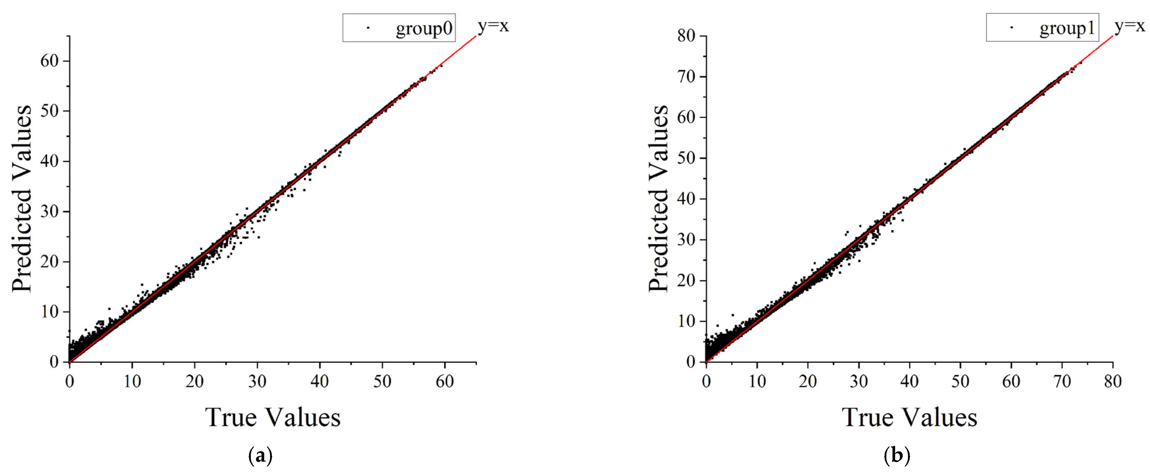
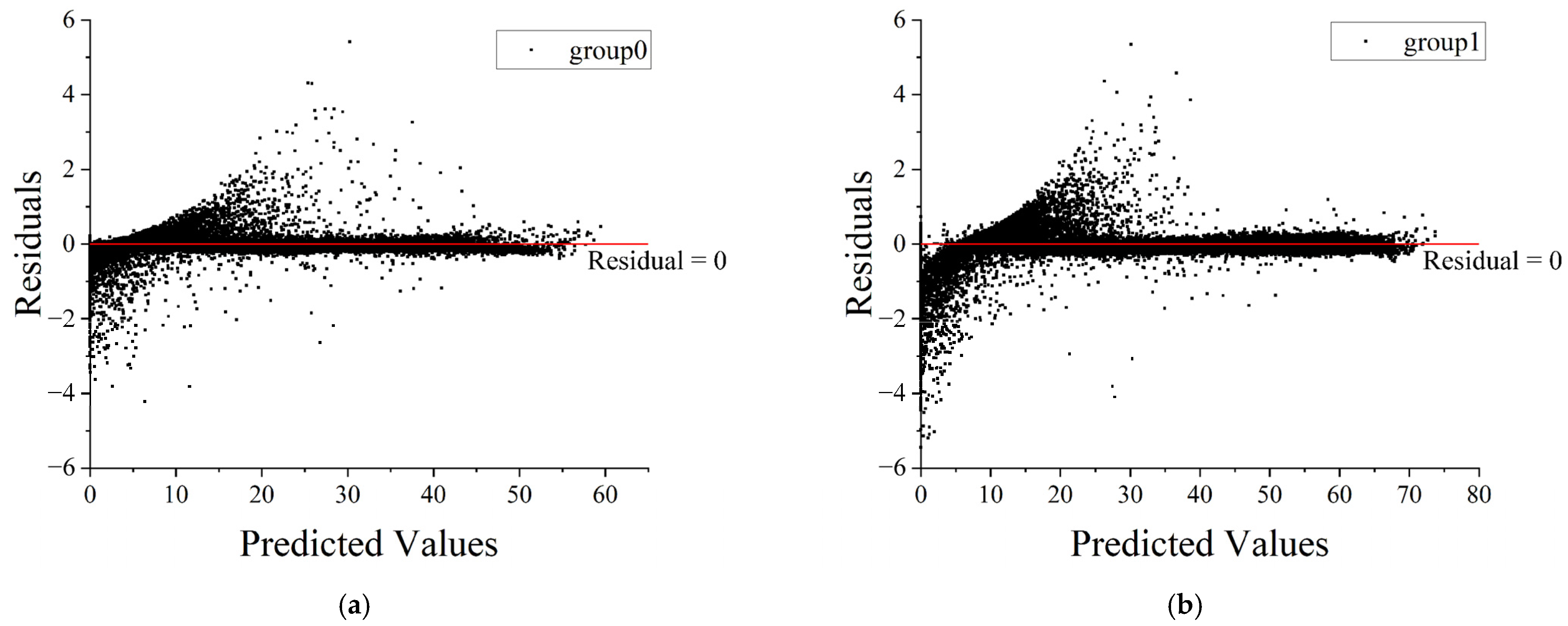
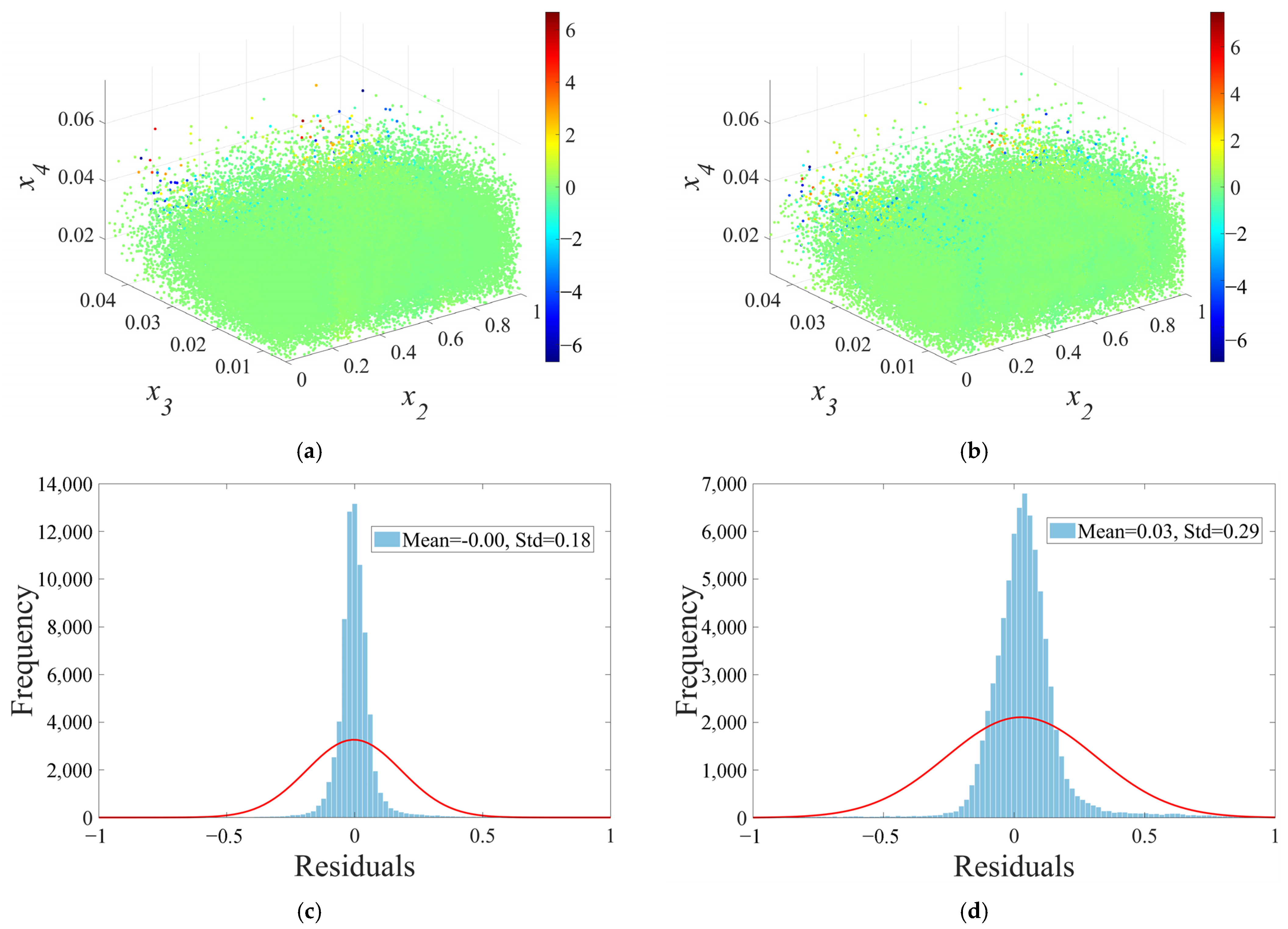
3.3. MATLAB Based Machine Learning Results
3.4. Analysis of Machine Learning Results
4. Conclusions
- (1)
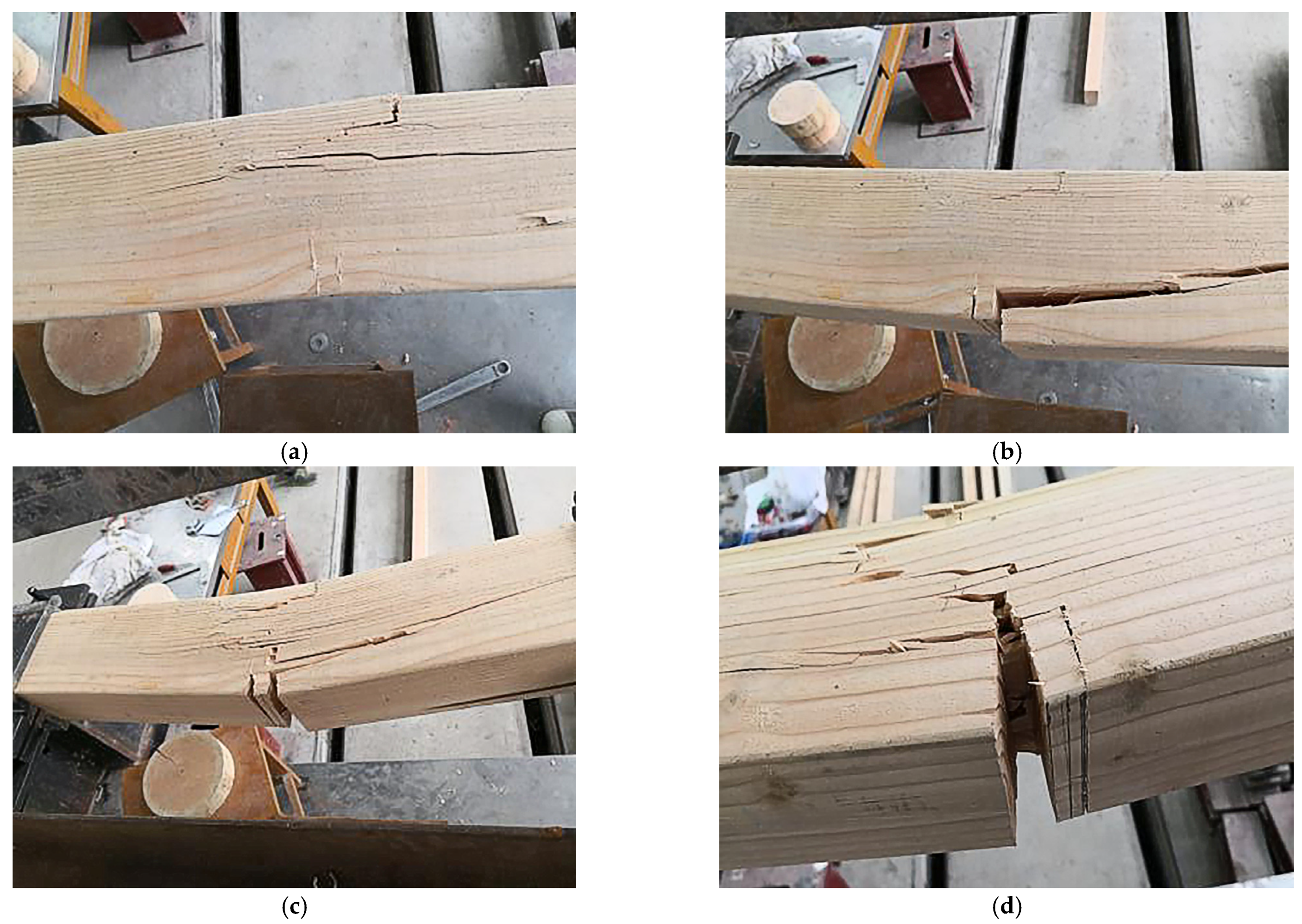
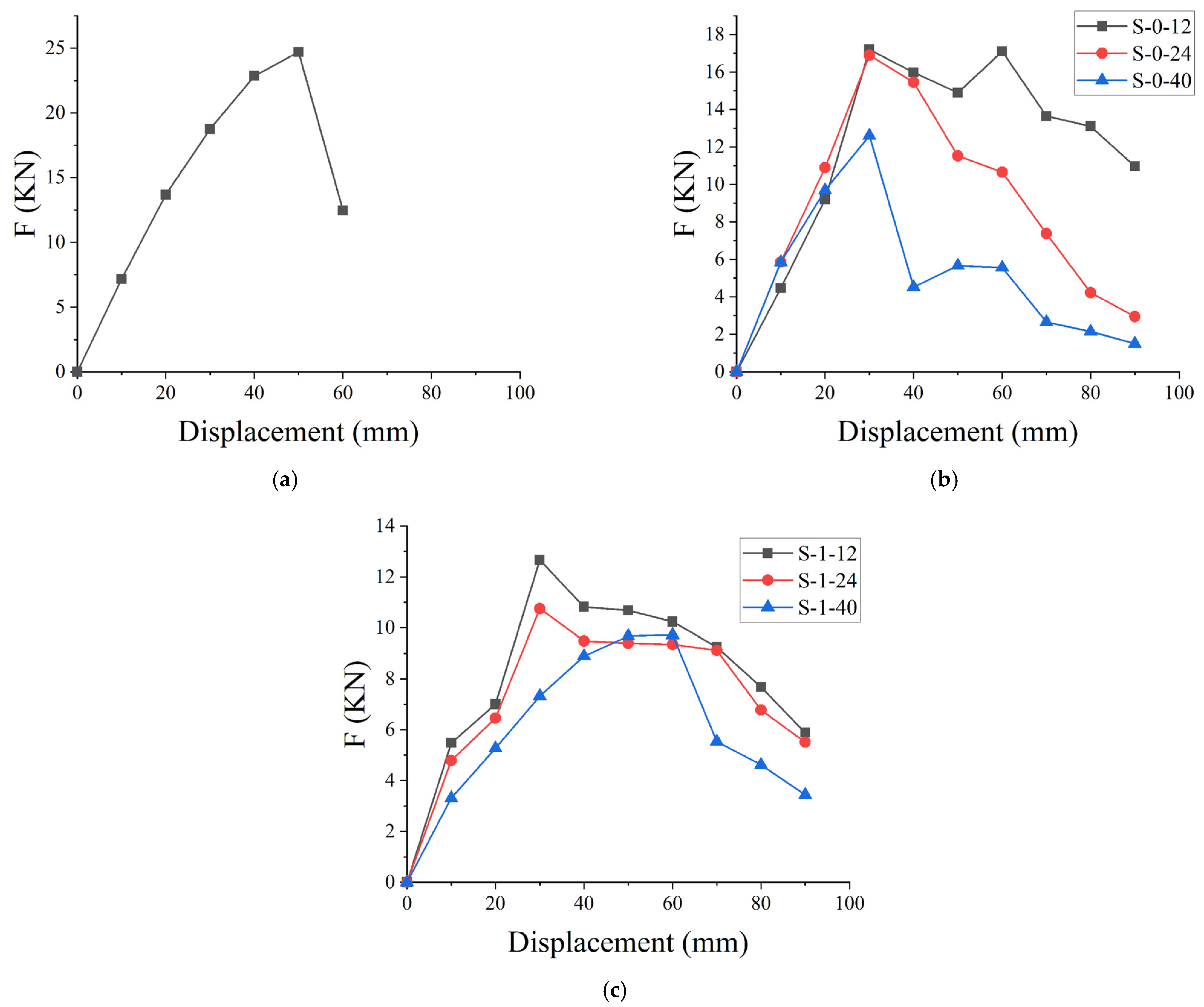
- Experimental verification of the timber knot weakening effect: Test results conclusively confirmed the significant weakening effect of timber knots on beam bearing capacity, particularly in the tension zone. Compared to defect-free beams, when knots were located in the compression zone, the ultimate bearing capacity decreased by 30.37% to 48.98%, representing a reduction of nearly one-third to half. When knots were situated in the tension zone, the reduction was even more pronounced, ranging from 48.71% to 60.64%, meaning a loss of nearly half to over sixty percent of capacity. Cracks preferentially initiated at defect sites caused by the knots, accelerating stiffness degradation.
- (2)
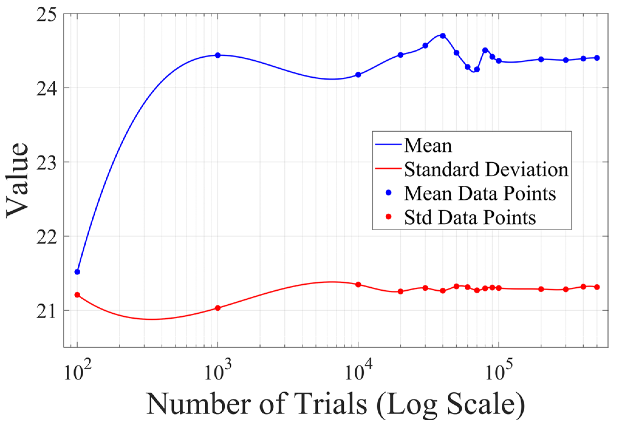
- Insights into random defect patterns from Monte Carlo simulations: A total of 3 × 500,000 Monte Carlo simulations were conducted to analyze the effects of defect randomness. The results reveal that timber knots in the tension zone exert a far greater impact on the beam’s bearing capacity than those in the compression zone. Specifically, when a knot is located at the mid-span of the tension zone, the maximum reduction in bearing capacity can reach a striking 75.67% (compared to a maximum reduction of 66.21% in the compression zone). Damage levels were classified into Class I, II, and III. For knots in the compression zone, Class III damage generally occurs within the 40–60% region of the normalized beam length. In contrast, for knots in the tension zone, Class III damage is distributed across a significantly wider range of 20–80%. Additionally, knots in the tension zone are more sensitive to capacity changes. Class I damage is typically distributed within 20% from the beam ends. For compression zone knots, Class II damage exhibits a bimodal distribution within the normalized length ranges of 0.2–0.4 and 0.6–0.8. Conversely, for tension zone knots, Class II damage is concentrated near the 0.2 and 0.8 marks, and these regions rapidly shrink as the knot parameters (diameter x3 and depth x4) increase.
- (3)
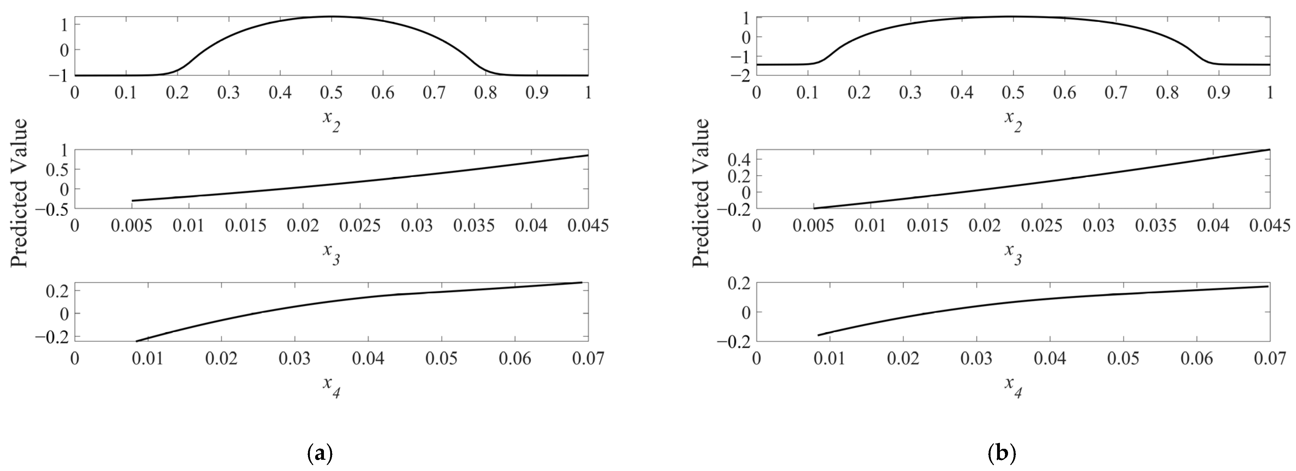
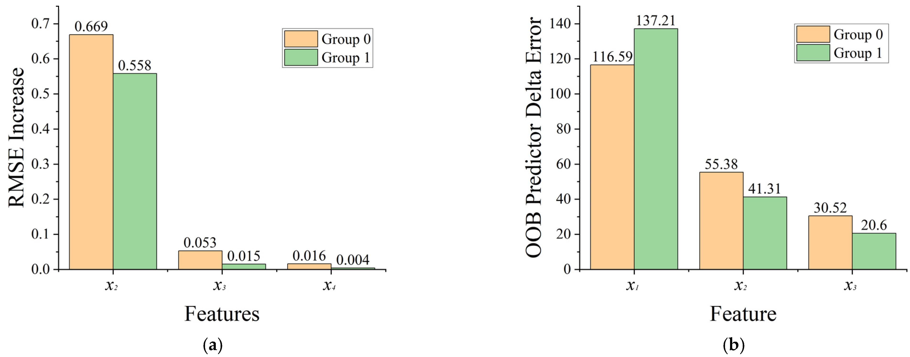
- Parameter sensitivity analysis via machine learning models: The fully connected neural network model identified the position of the timber knot (x2) as the dominant factor influencing the beam’s bearing capacity, with significantly higher importance than the knot’s diameter (x3) or depth (x4). The model further demonstrated that increasing the knot diameter (x3) weakens the bearing capacity in a convex pattern, indicating an increasing marginal weakening effect (i.e., each unit increase in diameter causes progressively greater capacity loss). Conversely, the influence of knot depth (x4) gradually plateaus, reflecting a decreasing marginal effect. These insights provide a comprehensive understanding of how different parameters affect the structural performance of timber beams with knots.
5. Future Works
- (1)
- In Monte Carlo simulations, knot diameters and depths are assumed to follow normal distributions, with parameters derived from Pan Yuchen’s thesis on timber knots in 16 wooden beams from Yangzhou’s Zhou Fujiu Mansion. This assumption may not hold across different tree species or engineering contexts.
- (2)
- While artificial timber knots simulate mechanical behavior, they inadequately replicate three-dimensional morphologies and fiber deviation effects and neglect factors like knot typology, wood grain orientation, and environmental aging.
- (3)
- The fully connected neural network’s performance heavily depends on the normality assumption, limiting its generalization capability for non-normally distributed knot parameters, complex 3D geometries, and multi-parameter interactions in diverse scenarios.
- (4)
- The model lacks explicit spatial modeling of knot position–size interactions, while its two-layer fully connected architecture risks overfitting on limited datasets.
- (5)
- Key simplifications include omitting 3D fiber deviations and annual ring distortions, assuming simply supported beams under uniform loads, and ignoring complex boundary conditions or stress–field superposition from multiple knots.
- (1)
- Data collection and model optimization: Centering on natural wood knot systems and modeling fidelity, short-term efforts will establish a geometric and material property database via batch CT scanning of natural wood specimens. Medium-term goals integrate statistical models of natural knots into the framework to evaluate prediction accuracy impacts. Long-term objectives compare artificial vs. natural knot model discrepancies to calibrate the framework and extend it to multi-factor analyses. Concurrently, machine learning attention mechanisms will capture joint distributions and nonlinear dependencies among knot parameters. MATLAB code documentation will be enhanced to enable open-source model sharing.
- (2)
- Model structure and algorithm improvement: Focusing on multi-scale physics integration, a cross-scale damage evolution model spanning “micro (fiber deviations, annual rings) to macro (structural mechanics)” will be developed. Integration of CT-scanned texture data will refine model accuracy. To improve knot simulation realism, solid modeling will simulate compression-zone knots, while layered modeling analyzes internal knots, strengthening the characterization of wood damage mechanisms.
- (3)
- Experimental design and validation: Prioritizing knot simulation technology, 3D printing techniques will replicate three-dimensional knot morphologies and fiber inclination characteristics, with mechanical equivalence verified via microscopic analysis. Experimental designs will distinguish live versus dead knot typologies and incorporate multi-factor variables (e.g., grain orientation, moisture content, microcracks) to ensure simulations reflect real-world complexity.
- (4)
- Engineering applications and scenario expansion: Addressing complex engineering demands, future work will investigate stress distributions under non-uniform loads and fixed/elastic supports, quantifying multi-knot stress-field superposition effects and cluster distribution impacts on load-bearing capacity. Case studies of Yangzhou’s heritage structures (e.g., Zhou Fujiu’s Residence, Wenchang Pavilion) will validate practical utility in heritage assessment. Benchmarking against international codes (Eurocode 5, NDS) will facilitate theory-to-practice translation. Additionally, long-term performance of knotted beams under creep–fatigue loads and environmental aging (humidity, temperature) will be studied to advance full-cycle analysis frameworks for engineering applications.
Author Contributions
Funding
Data Availability Statement
Conflicts of Interest
Nomenclature
| x1 | Knot position parameter (0 = compression zone, 1 = tension zone) |
| x2 | Normalized longitudinal position of the knot along the beam length (0 = beam end A, 1 = beam end B) |
| x3 | Knot diameter |
| x4 | Knot depth |
| Damage | Bearing capacity reduction rate (percentage) |
| S’ | Defect-free reference specimen |
| S-#-# | Numbering of defective specimens (the first # indicates the region: 0 = compression zone, 1 = tension zone; the second # indicates the depth. |
| RMSE | Root mean squared error (RMSE) (model evaluation index) |
| MAE | Mean absolute error (MAE) (model evaluation index) |
| R2 | Coefficient of Determination (R2) (model goodness-of-fit index) |
References
- Saad, K.; Lengyel, A. A parametric investigation of the influence of knots on the flexural behaviour of wood beams. Res. Sq. 2022. [Google Scholar] [CrossRef]
- Management Group for Timber Structure Design Code. Experimental study on axial compression of members of Yunnan pine and fir with wood knots. Metall. Constr. 1975, 56–71. (In Chinese) [Google Scholar] [CrossRef]
- Chang, C.-W.; Lin, F.-C. Strain concentration effects of wood knots under longitudinal tension obtained through digital image correlation. Biosyst. Eng. 2021, 212, 290–301. [Google Scholar] [CrossRef]
- Johansson, E.; Johansson, D.; Skog, J.; Fredriksson, M. Automated knot detection for high speed computed tomography on Pinus sylvestris L. and Picea abies (L.) Karst. using ellipse fitting in concentric surfaces. Comput. Electron. Agric. 2013, 96, 238–245. [Google Scholar] [CrossRef]
- Longuetaud, F.; Mothe, F.; Kerautret, B.; Krähenbühl, A.; Hory, L.; Leban, J.M.; Debled-Rennesson, I. Automatic knot detection and measurements from X-ray CT images of wood: A review and validation of an improved algorithm on softwood samples. Comput. Electron. Agric. 2012, 85, 77–89. [Google Scholar] [CrossRef]
- Zhong, Y.; Ren, H.; Lou, W. Experimental study on the effect of wood knots on the flexural strength of dimension lumber. J. Build. Mater. 2012, 15, 875–878. (In Chinese) [Google Scholar]
- Morrell, J.J.; Zabel, R. Wood strength and weight losses caused by soft rot fungi isolated from treated southern pine utility poles. Wood Fiber Sci. 1985, 17, 132–143. [Google Scholar]
- Guindos, P.; Guaita, M. The analytical influence of all types of knots on bending. Wood Sci. Technol. 2014, 48, 533–552. [Google Scholar] [CrossRef]
- Kandler, G.; Lukacevic, M.; Füssl, J. An algorithm for the geometric reconstruction of knots within timber boards based on fibre angle measurements. Constr. Build. Mater. 2016, 124, 945–960. [Google Scholar] [CrossRef]
- Baño, V.; Arriaga, F.; Soilán, A.; Guaita, M. Prediction of bending load capacity of timber beams using a finite element method simulation of knots and grain deviation. Biosyst. Eng. 2011, 109, 241–249. [Google Scholar] [CrossRef]
- Shi, B.; Zhang, X.; Ye, Y. The effect of wood knots on the bearing capacity of teeth of toothed-plate joints. Wood Ind. 2015, 29, 18–21. (In Chinese) [Google Scholar] [CrossRef]
- Ding, X.; Zhang, X. Effect of wood knots on the statistical properties of shear ductility of toothed-plate joints. For. Ind. 2016, 43, 21–25. (In Chinese) [Google Scholar] [CrossRef]
- Lukacevic, M.; Kandler, G.; Hu, M.; Olsson, A.; Füssl, J. A 3D model for knots and related fiber deviations in sawn timber for prediction of mechanical properties of boards. Mater. Des. 2019, 166, 107617. [Google Scholar] [CrossRef]
- Baño, V.; Arriaga, F.; Guaita, M. Determination of the influence of size and position of knots on load capacity and stress distribution in timber beams of Pinus sylvestris using finite element model. Biosyst. Eng. 2013, 114, 214–222. [Google Scholar] [CrossRef]
- Belz, J.; Kromoser, B. An Accessible Framework for Optimizing the Structural Performance of Wood-based Building Components. In Proceedings of the IASS 2024 Symposium: Redefining the Art of Structural Design, Zurich, Switzerland, 26–30 August 2024. [Google Scholar]
- Balzano, A.; Merela, M.; de Micco, V. Advances in Wood Anatomy: Cutting-Edge Techniques for Identifying Wood and Analyzing Its Structural Modifications. Forests 2024, 15, 1802. [Google Scholar] [CrossRef]
- Ehtisham, R.; Qayyum, W.; Plevris, V.; Mir, J.; Ahmad, A. Classification and Computing the Defected Area of Knots in Wooden Structures Using Image Processing and CNN. In Proceedings of the ECCOMAS Proceedia EUROGEN (2023), Chania, Greece, 1–3 June 2023. [Google Scholar]
- European Committee for Standardization. Eurocode 5: Design of Timber Structures; EN 1995 series; CEN: Brussels, Belgium, 2004. [Google Scholar]
- GB/T1929-2009; Methods of Sawing and Specimen Interception for Physical and Mechanical Specimens of Wood. Standard Press: Beijing, China, 2009. (In Chinese)
- GB1935-91; Test Method for Compressive Strength of Wood with Grain. Standard Press: Beijing, China, 1991. (In Chinese)
- GB1936-91; Test Method for Flexural Strength of Wood. Standard Press: Beijing, China, 1991. (In Chinese)
- GB/T15777-1995; Determination of Compressive Elastic Modulus of Wood with Smooth Grain. Standard Press: Beijing, China, 1995. (In Chinese)
- GB/T 50329-2002; Standard for Test Methods for Wood Structures. Building Industry Press: Beijing, China, 2002. (In Chinese)
- GB1928-2009; General Principles of Physical and Mechanical Test Methods for Wood. Building Industry Press: Beijing, China, 2009. (In Chinese)
- Li, F.; Wang, Q.; Chen, H.; Huang, Y. Initial test on flexural performance of BFRP-reinforced wooden beams. J. Huaqiao Univ. Nat. Sci. Ed. 2010, 31, 688–691. (In Chinese) [Google Scholar]
- EN 408:2010+A1:2012; Timber Structures-Structural Timber and Glued Laminated Timber-Determination of Some Physical and Mechanical Properties. European Committee for Standardization (CEN): Brussels, Belgium, 2012. Available online: https://standards.iteh.ai/catalog/standards/cen/6ffae6c9-5eaf-4c84-8bf3-5132cbfc563c/en-408-2010a1-2012 (accessed on 5 June 2025).
- Pan, Y. Research on the Effect of Damage on the Seismic Performance of Wooden Beams; Yangzhou University: Yangzhou, China, 2018. (In Chinese) [Google Scholar]

| Name | Tensile Strength Parallel to Grain (MPa) | Compressive Parallel to the Grain (MPa) | Compressive Strength Perpendicular to Grain (MPa) | Flexural Strength (MPa) | Flexural Modulus of Elasticity (MPa) |
|---|---|---|---|---|---|
| Average value | 93.82 | 34.2 | 6.0 | 87.88 | 13,500.24 |
| Standard deviation | 7.47 | 0.39 | 0.21 | 2.43 | 4.02 |
| Specimen’s Type | Elevation Views | Section Views | ||
|---|---|---|---|---|
| Defect-free specimen | 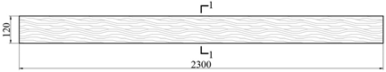 |  | ||
| Specimens containing defects | 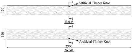 |  | ||
 |  |  | ||
| No | ① | ② | ③ |
|---|---|---|---|
| Parameter Value |
| Group | ① | ② | ③ |
|---|---|---|---|
| σ | 0.005 | 0.010 | 0.015 |
| x3 | 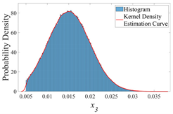 | 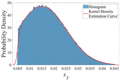 | 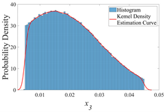 |
| x4 | 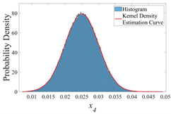 | 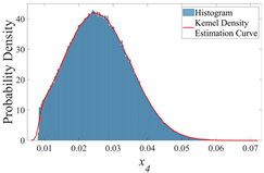 | 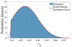 |
| Specimen | Yield Load (kN) | Breaking Load (kN) | Ultimate Load (kN) | Bending Moment at Ultimate Load (kN·m) | Percentage Decrease in Bearing Capacity (%) |
|---|---|---|---|---|---|
| S’ | 14.20 | 22.30 | 24.70 | 17.78 | - |
| S-0-12 | 13.40 | 15.30 | 17.20 | 12.38 | 30.37 |
| S-1-12 | 7.03 | 11.13 | 12.66 | 9.12 | 48.71 |
| S-0-24 | 11.60 | 13.30 | 16.90 | 12.17 | 31.55 |
| S-1-24 | 6.27 | 8.57 | 10.75 | 7.74 | 56.47 |
| S-0-40 | 9.10 | 10.50 | 12.60 | 9.07 | 48.98 |
| S-1-40 | 4.73 | 7.68 | 9.72 | 7.00 | 60.64 |
| Group | ① | ② | ③ |
|---|---|---|---|
| σ | 0.005 | 0.010 | 0.015 |
| x1 = 0 | 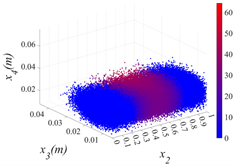 |  | 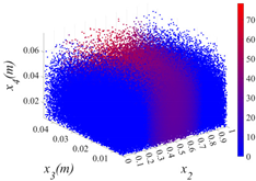 |
| x1 = 1 | 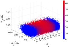 | 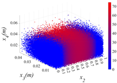 | 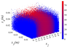 |
| Group | ① | ② | ③ |
|---|---|---|---|
| σ | 0.005 | 0.010 | 0.015 |
| x1 = 0 | 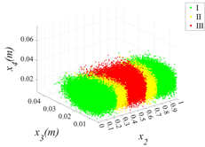 | 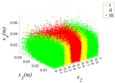 | 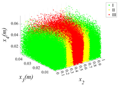 |
| x1 = 1 | 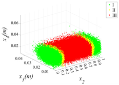 | 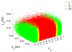 | 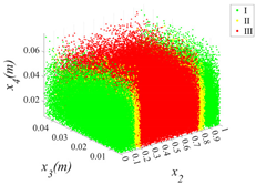 |
| Specimen | x1 | No | x2 | x3 | x4 | Damage (%) | Average (%) | Measured Results (%) | Absolute Error (%) |
|---|---|---|---|---|---|---|---|---|---|
| S-#-12 | 0 | ① | 0.5015 | 17.569 | 10.966 | 31.56 | 31.58 | 30.37 | +1.21 |
| ② | 0.4998 | 17.393 | 10.650 | 31.39 | |||||
| ③ | 0.4981 | 18.812 | 10.623 | 31.78 | |||||
| 1 | ① | 0.4989 | 18.111 | 11.900 | 53.89 | 53.86 | 48.71 | +5.15 | |
| ② | 0.5015 | 18.394 | 11.890 | 53.95 | |||||
| ③ | 0.4986 | 18.654 | 10.897 | 53.73 | |||||
| S-#-24 | 0 | ① | 0.5013 | 17.638 | 24.713 | 35.96 | 35.57 | 31.55 | +4.02 |
| ② | 0.4999 | 17.240 | 24.212 | 35.62 | |||||
| ③ | 0.5014 | 17.158 | 22.464 | 35.13 | |||||
| 1 | ① | 0.4985 | 17.066 | 23.516 | 56.10 | 56.49 | 56.47 | +0.02 | |
| ② | 0.5018 | 19.608 | 22.364 | 56.81 | |||||
| ③ | 0.5003 | 17.669 | 24.960 | 56.57 | |||||
| S-#-40 | 0 | ① | 0.4989 | 20.806 | 40.970 | 41.23 | 40.45 | 48.98 | −8.53 |
| ② | 0.5007 | 20.357 | 39.925 | 40.74 | |||||
| ③ | 0.4984 | 18.379 | 41.026 | 39.38 | |||||
| 1 | ① | 0.4999 | 19.373 | 40.906 | 59.35 | 59.33 | 60.64 | −1.31 | |
| ② | 0.5002 | 19.190 | 39.741 | 59.15 | |||||
| ③ | 0.5005 | 19.589 | 41.213 | 59.48 |
| Group | ① | ② | ③ |
|---|---|---|---|
| σ | 0.005 | 0.010 | 0.015 |
| Cumulative Probability | 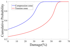 | 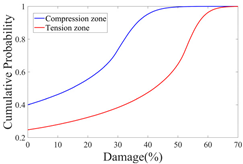 |  |
| Probability Density | 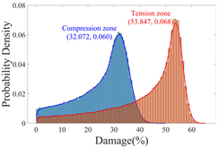 | 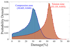 | 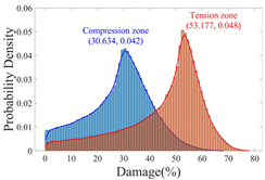 |
| RMSE | MAE | R2 | |
|---|---|---|---|
| Group 0 (x1 = 0) | 0.20368 | 0.085381 | 0.99983 |
| Group 1 (x1 = 1) | 0.28641 | 0.13161 | 0.99984 |
Disclaimer/Publisher’s Note: The statements, opinions and data contained in all publications are solely those of the individual author(s) and contributor(s) and not of MDPI and/or the editor(s). MDPI and/or the editor(s) disclaim responsibility for any injury to people or property resulting from any ideas, methods, instructions or products referred to in the content. |
© 2025 by the authors. Licensee MDPI, Basel, Switzerland. This article is an open access article distributed under the terms and conditions of the Creative Commons Attribution (CC BY) license (https://creativecommons.org/licenses/by/4.0/).
Share and Cite
Wang, P.; Liu, G.; Li, F.; Li, S.; Milani, G.; Abruzzese, D. Assessment of Knot-Induced Degradation in Timber Beams: Probabilistic Modeling and Data-Driven Prediction of Load Capacity Loss. Buildings 2025, 15, 2058. https://doi.org/10.3390/buildings15122058
Wang P, Liu G, Li F, Li S, Milani G, Abruzzese D. Assessment of Knot-Induced Degradation in Timber Beams: Probabilistic Modeling and Data-Driven Prediction of Load Capacity Loss. Buildings. 2025; 15(12):2058. https://doi.org/10.3390/buildings15122058
Chicago/Turabian StyleWang, Peixuan, Guoming Liu, Fanrong Li, Shengcai Li, Gabriele Milani, and Donato Abruzzese. 2025. "Assessment of Knot-Induced Degradation in Timber Beams: Probabilistic Modeling and Data-Driven Prediction of Load Capacity Loss" Buildings 15, no. 12: 2058. https://doi.org/10.3390/buildings15122058
APA StyleWang, P., Liu, G., Li, F., Li, S., Milani, G., & Abruzzese, D. (2025). Assessment of Knot-Induced Degradation in Timber Beams: Probabilistic Modeling and Data-Driven Prediction of Load Capacity Loss. Buildings, 15(12), 2058. https://doi.org/10.3390/buildings15122058