Abstract
In northern China, radiant floor heating is widely used in multi-apartment residential buildings, with indoor temperature being a key factor in evaluating a user’s heating demands. However, due to variations in building structure, room orientation, and the outdoor environment, identifying the optimal placement of temperature sensors across multiple zones remains challenging. In this study, we propose a data-driven methodology to identify the optimal placement of temperature sensors for a typical apartment with multiple zones. The proposed methodology is based on computational fluid dynamics (CFD) simulations of several typical scenarios and quantifies the relationship between the temperature field and the volume-averaged operating temperature to determine the optimal locations for temperature sensors. Results indicate that the temperature sensors need to be placed on planes ranging from 1.0 m to 1.7 m, with each plane featuring a distinct optimal area. The RMSE analysis reveals that, despite obvious temperature variations across the residence, the root mean square errors (RMSEs) at the designated sensor locations remain consistently low, with a maximum of 0.35 °C and most values below 0.3 °C. The above results indicate that the optimal sensor placement can significantly reduce potential errors between recorded temperatures and volume-averaged operating temperatures, which can be used as input parameters for personal indoor temperature control.
1. Introduction
In recent years, radiant floor heating systems have become increasingly popular in northern China as an energy-efficient and comfortable indoor heating method. These systems utilize radiant heat transfer from the floor surface to objects and occupants within the indoor space, providing a uniform and comfortable thermal environment compared with traditional heating methods. It was reported that energy savings of 27–59% could be achieved while maintaining an equivalent comfort level [1,2]. Since 2003, China has initiated the implementation of a heat metering reform. Compared with the traditional billing system based on the heated area, the heat metering and billing mode encourage people to adjust the room temperature based on their actual needs, thus reducing heating consumption. Heat metering and the need for personal control have driven the development of a temperature monitoring system, supported by Internet of Things (IoT) technology.
Temperature sensors installed indoors need to accurately reflect the thermal comfort of occupants. However, due to differences in orientation and structure, significant temperature variations may occur between different zones in an apartment. Particularly, individuals in rooms directly exposed to solar radiation will experience higher temperature compared with those in shaded rooms [3]. Optimal sensor placement (OSP) is a critical research area in building engineering, aiming to maximize the effectiveness of monitoring systems (e.g., structural health, indoor environment, energy, security) while minimizing cost and complexity. Various methods can address this issue, including model-based approaches, data-driven techniques, and optimization algorithms [4,5].
Previous research has examined the impact of sensor placement on building performance and the effects of various sensor types on the efficiency of an HVAC (heating, ventilation, and air conditioning) system [6,7]. Existing standards, such as ASHRAE (American Society of Heating, Refrigerating and Air-Conditioning Engineers) Standard 55 [8], do not provide specific guidelines for sensor placement for a radiant floor heating system, and temperature sensors currently installed in practice often fail to accurately reflect thermal comfort. To address this issue, optimizing sensor placement across multiple zones is essential for efficient and practical temperature management. Several researchers have explored various methods for determining optimal sensor placement for indoor environment evaluation [9,10] or air quality [11,12], with data-driven approaches being particularly prominent. Yoganathan et al. [13] introduced a data-driven method employing clustering algorithms and the Pareto principle to identify optimal sensor measurement points in office buildings. Their study revealed that the optimal sensor positions for temperature and humidity varied over time and space. Suryanarayana, G et al. [14] developed a data-driven method for optimal sensor placement in multi-zone buildings, leveraging statistical tests to analyze interdependencies among available sensor measurements.
For multi-apartment buildings containing hundreds of households, the predominant type in cities in northern China, room temperatures are required to evaluate and control the thermal state for each apartment [15]. However, deploying and maintaining numerous sensors can be costly and involve a significant amount of work. For a single apartment with multiple zones, cost constraints often lead engineers to install a single sensor rather than multiple sensors, as the latter calls for larger maintenance expense and installing space [16]. In such cases, careful considerations of sensor number and locations are crucial for accurately capturing the overall thermal comfort of the apartment. Many prior studies have concentrated on minimizing the number of sensors required or optimizing the placement under limited number [17,18,19,20,21]. Ren and Cao [22] employed a minimal number of sensors to track indoor pollutant concentrations. The prediction model achieved satisfactory performance with as few as five sensors. Kyriacou et al. [23] developed a toolbox for sensor placement and contaminant monitoring in multi-zone buildings by solving a multi-objective optimization problem for a specified number of installed sensors.
Data-driven approaches require a large amount of data for model training, but acquiring extensive indoor temperature data for residential users proved highly challenging. Accurate information on the thermal environment and airflow patterns can be provided by computational fluid dynamics (CFD) simulations, involving a discretization process in both space and time, as well as an iterative solution of mass, momentum, and energy conservation equations [24,25]. In previous studies, CFD models were employed to generate a substantial amount of indoor temperature data, which were then combined with other approaches to determine the optimal positions for temperature sensors in ventilation and air conditioning systems [26,27,28,29]. A key advantage of this approach was that it eliminated the need to install numerous temperature sensors in confined spaces, which is intrusive and potentially disruptive of the occupants’ activities. Tian et al. [30] proposed an optimization platform by coupling simulations of airflow and an HVAC system, which was used to determine the optimal positions of thermostats. Du et al. [31] attempted to optimize sensor placement based on coupled simulations of HVAC systems and indoor thermal environments to find the placement of temperature sensors. Li et al. [32] proposed a high spatial resolution indoor temperature field reconstruction and estimation based on finite sensors. The primary features of the indoor temperature field under steady-state/dynamic conditions were obtained using proper orthogonal decomposition. Jiang et al. [33] provided a two-stage physical field reconstruction method to quickly rebuild an indoor physical field by combining observation input parameters from CFD simulations and sparse observations of the field. Chen and Gorlé [34] proposed a novel method using CFD simulations with uncertainty quantification to optimize the placement of temperature sensors in buildings with buoyancy-driven natural ventilation, ensuring that the measured results represent the volume-averaged temperature while also supporting the analysis of spatial variations in temperature fields.
Previous studies on radiant floor heating primarily focused on optimizing flow fields and system layouts, with limited attention given to optimizing sensor placement. This was because most heating systems’ control strategies relied feedforward or predictive control adjustments [35,36], or were adjusted based on historical operation data or experiences of the practitioner [16]. These control strategies often led to user-side temperature mismatch issues due to hydraulic and thermal imbalance. The use of end-user indoor temperatures for control was rarely applied in radiant heating systems, due to the nonuniform distribution of air temperature and the effects of radiation.
Few studies have been conducted on the optimization of sensor placement in residential buildings with radiant floor heating. Most optimization efforts for sensor placement focus on indoor natural convection or forced convection to account for the impact of airflow and temperature distribution, without considering the influence of floor radiation and solar radiation. In radiant heated space, besides the air temperature, the radiant heat exchange between occupants and the inner surfaces of the surrounding enclosure also affect the thermal sensation of occupants. The nonuniform thermal radiation field needs to be incorporated into the process of sensor placement optimization. On the other hand, the continuous changes in outdoor temperature and solar radiation during the heating season cause the optimal sensor locations to constantly shift. The optimal measurement points at one moment may become entirely unsuitable at another.
This study aims to identify the optimal sensor placement strategy for assessing thermal comfort in a typical multi-apartment residential building, considering the impact of floor heating and solar radiation. First, by modeling seven representative time points per day for three typical days during the heating season, the influence of outdoor temperature and solar radiation on the indoor environment was taken into account. The operating temperature was used to characterize the thermal sensation of occupants under radiant floor heating. Second, the absolute temperature difference between sensor location and occupied zone was employed to quantitatively assess whether the air temperatures at various locations can effectively represent the average operative temperature of an occupied zone. The average difference at different times was used to evaluate the overall deviation, while the maximum difference was used to account for extreme local deviations. Third, after preliminary screening with a temperature difference threshold of 0.25 degrees, a comprehensive evaluation index was proposed by considering both the mean and maximum temperature difference across time. This led to the development of the quantitative indicator , which accurately represents the actual thermal sensation of the designated active zones and offers a reliable reference for determining sensor placement in a radiant heating system. By cross-selecting the standard deviation and mean value of for zones 1 to 9, the optimal sensor locations on different planes were determined.
2. Numerical Modeling
2.1. Information on Apartment
The investigated apartment is part of a typical multi-apartment residential building located in Shenyang (123.3° E, 41.8° N), China. The building has a total floor area of 5800 m2, with seven above-ground floors. The first level serves as a garage, with residential units occupying the second through seventh floors. Each floor has three units, and each unit contains two apartments. The apartment selected for this study is located on the third floor of the building, in the westernmost end, with a floor area of 120 . As illustrated in Figure 1, the apartment consists of three bedrooms, a living room and bathroom, and a kitchen. The enclosing structure and material properties are listed in Table 1. A detailed construction of the floor is provided in Figure 2. The materials of the floor structure from top to bottom are granite, cement mortar, fine stone concrete, and polystyrene insulation. Since the thermal conductivities of the top 3 layers differ very little, they are simplified into a single layer [37]. Due to the insulating effect of the bottom layer, heat transfer downward through the floor is neglected.
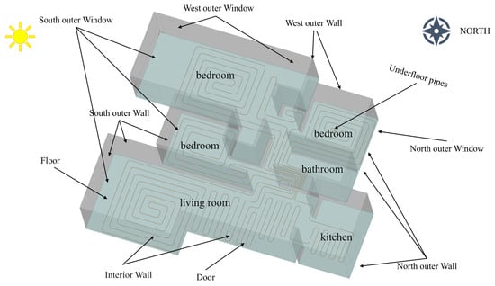
Figure 1.
Detailed description of the apartment in this study.

Table 1.
Solid material properties.
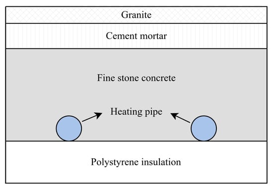
Figure 2.
Floor structure.
The building is heated by a central heating system, with fluid-filled pipes buried underground as heating terminal device. As Figure 1 shows, the radiant floor heating system consists of six branches. The hot water provided by the central heating system is supplied from the manifold to the floor of each room, then returns to the collector and back to the heating exchange station. As a result, the floor surface is heated, generating natural convection between the floor and the air, as well as radiant heat exchange between the floor and the surrounding walls. This heating method requires a much lower water temperature to achieve the same effect compared with traditional radiator heating. The building design fully complies with relevant Chinese standards and regulations. The material of the heating pipe is cross-linked polyethylene. The pipe diameter is 20 mm, with a wall thickness of 2.0 mm. The pipes is adopted in a spiral layout, with a spacing of 20 cm between adjacent pipes. The water flow velocity in the pipes ranges from 0.25 to 0.5 m/s.
In the floor heating system, hot water transfers heat to the pipes through convective heat transfer, which is then further conducted to the floor in the form of thermal conduction. This leads to an increase in the surface temperature of the floor. The heat transfer process at the floor surface consists of two parts: (1) The floor surface transfers heat to the nearby air via convective heat transfer, inducing natural convection in the room and distributing heat to other areas indoors. (2) The floor surface emits thermal radiation, which is absorbed by the human body and other indoor surfaces. The radiant heat absorbed by the human body enhances thermal comfort, while the heat absorbed by other surfaces raises their temperature, causing them to further emit heat through convection and radiation.
For multi-apartment buildings, prior research has demonstrated significant variations in heat transfer and temperature differences across diverse locations. In order to assess the overall comfort of the apartment, a thorough evaluation of each room is required. However, in practice, room temperature monitoring faces limitations due to budget constraints and user reluctance. A limited number of measurement points make it difficult to accurately reflect the overall comfort level of the apartment [38,39,40]. Nine active zones are defined as in Figure 3. The optimal sensor location needs to reflect the overall thermal comfort across all defined zones. In order to validate numerical simulation, experimental measurements were conducted during the heating season. Air temperatures at different heights (0.5 m, 1.0 m, 1.5 m, 2.0 m, and 2.5 m) and locations (labeled as A, B, and C in Figure 3) were measured using four-wire PT100 temperature sensors (PT100 WZP, Asmik, Hangzhou, China) with an accuracy of 0.1 °C and collected using a recorder (MIK-R200D, Asmik, Hangzhou, China) at 5 min intervals.
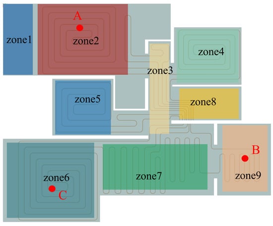
Figure 3.
The zoning and monitoring points within the apartment.
2.2. Modeling Approach
2.2.1. Computational Domains
The whole computational domain was divided into eight regions consisting of a fluid domain for indoor air, a solid domain for concrete floor, and six fluid domains for underground pipes filled with water. For fluid domains, continuity, momentum, and energy conservation equations were solved to capture the physics of the flow field, as shown in the following Equation (1):
where is a generic variable, representing unity in continuity equation, in momentum equation, and h in energy equation. is the digression coefficient and is the source term. To reasonably simplify CFD simulation process, the following assumptions were made in this work: (1) The flow field in each scenario was steady, fully developed, and turbulent. (2) Indoor air and water in pipes were considered incompressible under all scenarios. (3) The material properties of the floor were assumed to be isotropic and homogeneous. (4) The thermal conduction resistance of the pipes was neglected, as well as the contact thermal resistance between pipes and the floor.
In order to account for the natural convection in the air domain, the effect of buoyancy was modeled using Boussinesq approximation. The RNG k- turbulent model has proven to be a robust, well-functioning model in predicting indoor airflow characteristics when compared with other two-equation models [41,42,43,44]. Previous studies concluded that it was one of the best approaches for exploring bluff body flows [45,46,47,48] and studying natural ventilation [49,50,51]. In this work, to accurately simulate the airflow between adjacent zones and the natural convection induced by floor heating, the RNG k- model is employed for turbulence approximation.
For a solid domain, only the energy equation was solved to predict the heat conduction, as shown in the following Equation (2):
where is the solid enthalpy, and is the solid heat diffusivity.
2.2.2. Radiation Model
The discrete ordinates (DO) radiation model was employed in the air domain to consider the radiative heat transfer, based on the validated hypothesis that the air is a non-participating radiation medium [52]. The DO model discretizes the radiation in space into numbers of solid angles, solving radiative intensity transport equation at each angle. In this study, the space was discretized into 12 azimuthal angles and 6 angular angles, leading to 72 radiative intensity transport equations in total. The incident radiation field was calculated to take into account the influence of radiant heat transfer on the thermal environment, as shown in the following Equation (3):
where G describes the incident radiation in W/m2, I is the radiative intensity in a specific direction, and is the solid angle.
The mean radiant temperature (MRT) was calculated using Equation (4), with its variability influenced by spatial and temporal factors, as experimentally and numerically validated [53]. Air temperatures and mean radiant temperatures were collected at distances of 10–20 cm from the wall surface. This range aligns with the operational limits of most temperature sensors, which are typically unable to measure radiation directly and are sensitive to spatial positioning.
where () is the Stefan–Boltzmann constant.
The solar radiation was also taken into account, with a solar calculator and ray tracing algorithm to determine the sunray’s direction and intensity. The minimum inputs required by the solar calculator are global location, start date and time, geometric orientation, and sky cloud cover fraction. Then, the solar calculator provides outputs such as solar direction vectors and decomposes solar radiation into direct radiation on the Earth’s surface, diffuse radiation on vertical and horizontal surfaces, and ground-reflected radiation on vertical surfaces.
2.2.3. Meshing
The cell type for the mesh was hexahedral, with a minimum cell size of 0.015 m for the air domain and 0.002 m for the floor layer and underfloor pipe domains. Figure 4, Figure 5 and Figure 6 show the mesh generation for the air domain, floor domain, and pipe domains, respectively, with 1.36 million cells for the air domain, 14.97 million cells for the floor layer, and 12.5 million cells across all the pipe domains. During meshing, mesh refinement was performed at the contact surfaces between different domains.
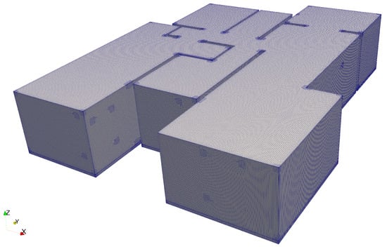
Figure 4.
Mesh for the air domain.
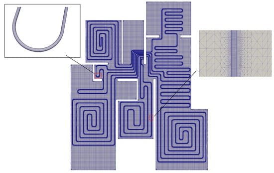
Figure 5.
Mesh for the floor domain.
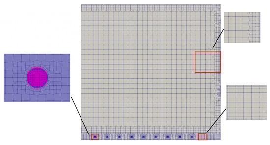
Figure 6.
Mesh for the pipe domains.
The floor heat flux and air velocity in the x direction in the air domain were extracted to check mesh independence, as shown in Figure 7. When the number of cells reaches 1.36 million, the velocity field and floor heat flux stabilize and remain stable. Thus, 1.36 million cells were chosen for the air domain to balance computation time and improve precision.
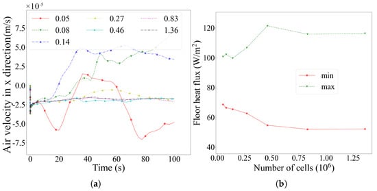
Figure 7.
Floor heat flux and air velocity in the x direction from a mesh independence study: (a) air velocity variation over time in the x direction corresponding to different cell numbers () and (b) floor heat flux at 100 s.
2.2.4. Boundary Conditions
Considering the spatial and temporal variability of the indoor environment, simulations were conducted for three typical weather conditions, representing the coldest, warmest, and intermediate periods of the heating season. Both daytime and nighttime scenarios were evaluated, with the assumption of a sunny weather, resulting in a total of six simulated scenarios in each condition.
Figure 8 shows the line graphs depicting outdoor temperatures and supply water temperatures over time for three weather conditions. These serve as input parameters for the outdoor temperature in the convective boundary of the building envelope and the supply water temperature for the radiant floor heating system. Table 2 lists the fluid physical parameters, and Table 3 lists the boundary settings of the model.
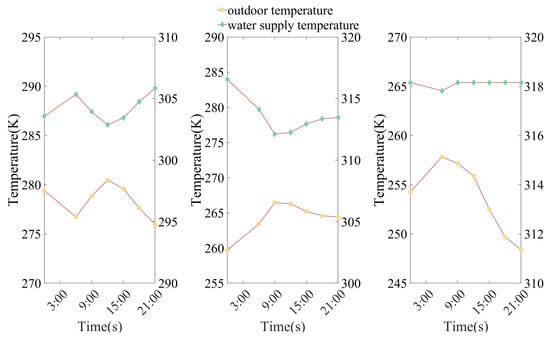
Figure 8.
Outdoor air temperature and supply temperature profiles in selected days.
Table 2.
Fluid properties’ parameters.
Table 3.
Boundary conditions for CFD simulation.
For the contact interface between the air domain and the floor layer, a mixed boundary condition was employed, which comprehensively considers the medium properties and heat transfer processes on both sides of the interface to obtain the boundary surface temperature, as shown in the following Equation (5):
where and are the convective and radiative heat transfer, respectively, at the floor surface of the air domain, and is the conductive heat transfer at the floor surface of the floor domain.
For radiation boundary conditions, it is considered that the radiation rays leaving a wall include both the radiation rays emitted by itself and the reflection of all the incident radiation. For solar radiation, windows were considered transparent. The solar rays passing through the windows were incorporated into the ray equation of the closest direction, accounting for the impacts of solar radiation on wall temperatures.
2.2.5. Solver Settings
The pressure-velocity coupling adopted the SIMPLE (Semi-Implicit Method for Pressure Linked Equations) algorithm. Second-order discretization schemes were employed for both the convection terms and the viscous terms of the above conservation equations, while gradients were computed using the Least-Squares-Cell-Based Method. The solutions were considered converged when the scaled residuals were less than 10−6 for the energy equation and 10−4 for the remaining equations. Initially, the energy and momentum equations were solved for both the air domain and the pipe domains. In order to save computational time, the flow fields in underfloor pipes were frozen once a steady state had been reached, and only the indoor air and concrete floor regions were simulated.
To ensure that the simulation results comprehensively cover typical operating conditions at different times of the day, seven representative time points (0:00, 6:00, 9:00, 12:00, 15:00, 18:00, and 21:00) within a day were selected, corresponding to varying outdoor temperatures and supply water temperatures of floor heating, thereby establishing seven distinct simulation scenarios. In order to further investigate the influence of the weather condition and solar radiation on the indoor environment, three typical days (1 November, 12 December, and 24 January) in different heating stages were selected to repeat the simulation process, obtaining a total of 21 independent sets of simulation data.
After the simulations, datasets required for sensor location optimization were extracted: (1) the air temperature field at 0.1 m, 0.6 m, 1.0 m, 1.5 m, 1.7 m, and 2.0 m planes at each moment, and (2) the flow fields for the 9 zones, including incident radiation, air temperature, and velocity.
3. Optimization Method for Sensor Placement
For the floor heating system, the heat flux on the floor surface can be controlled by adjusting the supply water temperature or flow rate. Unlike air conditioning systems, floor heating lacks rapid response rates and immediate adjustability, resulting in significant latency and a slow response time. In central heating systems in China, the supply temperature and flow rate are commonly controlled at heat exchange stations based on experience. Meanwhile, widespread complaints about a cold indoor temperature prompt a significant increase in the supply temperature or flow rate to address the issue. These practices highlight two key problems. First, users’ actual heat demand cannot accurately be assessed without indoor temperature monitoring. Second, central adjustments often lead to system imbalances and may cause overheating for some users, prompting users to open windows for cooling, thus resulting in excessive energy waste. Addressing these challenges requires collecting accurate room temperature data from users. However, most commercially available sensors are encased in shells, allowing only the measurement of convective heat transfer, failing to account for radiation effects, which contribute to 50% of human thermal comfort. Furthermore, there are no established standards for optimal sensor placement, and temperature data collection often relies on experiences or users’ subjective decisions for sensor installation.
Flow fields generated from CFD modeling were used to calculate the volume-averaged operating temperatures, as well as at different horizontal planes. Then the metrics for quantities of interest (QoIs) were derived and used to identify the optimal sensor location by defining the representativeness of the measurement point temperature for zone thermal comfort. The mean value and standard deviation of the metrics were calculated and crossed to determine the optimal sensor locations. Figure 9 illustrates the proposed workflow.
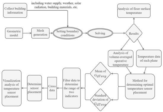
Figure 9.
Workflow of the presented methodology.
3.1. Operative Temperature
Operative temperature is a single index to estimate thermal sensation, which combines the effects of convective and radiative heat transfer, as defined in ASHRAE Standard 55 [8]. With the air temperature and MRT derived from the above simulations, operative temperature can be calculated according to the following Equation (6):
where represents the operative temperature, is the air temperature, and is the mean radiant temperature (MRT). The parameter A can be obtained from Table 4, where denotes the air velocity.
Table 4.
Relationship between A and .
3.2. Quantities of Interest for Selecting Sensor Locations
3.2.1. Absolute Temperature Difference Between Sensor Location and Occupied Zone
To quantitatively assess whether the air temperatures at various locations on different height planes can effectively represent the average operative temperature of an occupied zone, a method based on the analysis of absolute temperature difference was proposed, aiming to identify the most representative temperature sensor locations that best reflect occupant thermal sensation.
The detailed assessment steps are as follows:
- 1.
- Using the previously extracted air temperature field, the absolute temperature difference between each location and the volume-averaged operative temperature of the specified zone was calculated as Equation (7) to evaluate the extent to which the location can approximate the actual occupant thermal sensation. The smaller the difference, the more accurately the air temperature at that location can reflect occupant thermal sensation, thereby demonstrating its potential as a representative temperature measurement point.where is the air temperature at a specified coordinate position on a plane at a height of h, is the volume-averaged operative temperature in the zone of interest (denoted by j), and represents the simulation scenario corresponding to different times.
- 2.
- To comprehensively characterize the representative temperature features across different times within a typical day, the statistical average above temperature differences for all seven typical time points was calculated as follows:where is the total number of scenarios in a day.With this evaluation metric, the temperature deviation levels of various locations can be quantitatively evaluated on a temporal dimension. The smaller the mean absolute temperature difference, the more consistently the location temperature aligns with the average operative temperature of the occupied zone throughout the day. This indicates stronger representativeness, making it suitable for placement as an indoor temperature monitoring point.
- 3.
- In practice, localized thermal environments may experience significant fluctuations at certain times—such as sudden temperature rise caused by solar radiation. To identify areas with potential deviation risks, the maximum absolute temperature difference was employed as a second evaluation metric. The absolute temperature difference values across all times are extracted, and the maximum value is calculated and defined as as in Equation (9).The introduction of this metric aims at identifying and excluding locations with abnormal temperature or significant thermal environment fluctuations at certain times, thereby ensuring the robustness and long-term effectiveness of the subsequent optimal sensor location selected. By combining it with the analysis of average temperature differences, a more comprehensive evaluation can be achieved regarding the temporal consistency and spatial representativeness of air temperatures.
3.2.2. Criterion for Selecting Sensor Locations
Based on the aforementioned temperature difference analysis, a simple threshold method for the absolute temperature difference was employed, integrating both the average and maximum temperature differences over the time dimension.
- 1.
- Preliminary Screening Based on Absolute Temperature Difference ThresholdFirst, the absolute temperature difference threshold is set to 0.25 °C, which is determined based on human sensitivity to thermal environment changes. If the absolute temperature difference between a specified location and the average operative temperature of the occupied zone remains below 0.25 °C across all seven typical scenarios, the thermal sensation at this location is essentially consistent with that of the occupied zone, classifying it as the zone with stable temperature distribution. Consequently, such a location is considered highly representative and is assigned a comprehensive evaluation index value of 0.
- 2.
- Further Evaluation Based on Mean and Maximum Temperature DifferencesFor locations that do not meet the preliminary screening criteria, further analysis of their temperature fluctuation amplitude is required. Considering that some locations may closely align with the zone operative temperature most of the time but exhibit significant deviations in certain instances, it is necessary to comprehensively evaluate their representativeness by considering both the mean temperature difference (indicating overall deviation) and the maximum temperature difference (indicating extreme local deviations) across time.Therefore, the comprehensive evaluation index for such locations is defined as follows:This criterion aims to identify localized temperature anomalies caused by variations in outdoor conditions or water supply temperatures over time. By imposing dual constraints on both the extreme and mean temperature differences, it effectively eliminates misleading locations that exhibit severe deviations in certain instances while appearing generally well behaved overall.
3.2.3. Normalization and Quantitative Indicator Calculation
In a real thermal environment, the following scenario may arise: the absolute temperature difference at all monitoring locations exceeds 0.25 °C, meaning none of the measurement locations meet the criteria for representativeness. This phenomenon may result from nonuniform distributions of heat transfer, airflow, or load. To identify the optimal sensor location under such circumstances, a normalized quantitative evaluation method was proposed.
By normalizing the above evaluation index of a certain plane relative to the maximum index value on that plane, a new dimensionless quantitative index is defined, calculated as follows:
The resulting normalized metric ranges from 0 to 1, with lower values indicating higher sensitivity in reflecting the volume-averaged operative temperature of the zone. The smaller the normalized index of a certain spatial location, the smaller the temperature difference deviation on the relative scale, indicating closer proximity to the actual thermal environment of the occupied zone. Therefore, to ensure accurate verification of these temperature measurements, sensors should be positioned in areas with lower values. The sensitivities of volume-averaged temperatures across all nine zones (described in Figure 3) were calculated and compared to determine the optimal sensor location.
4. Results and Discussion
4.1. Analysis of Temperature Distribution
4.1.1. Vertical Temperature Profiles
A comparison between the simulated and measured values of air temperature at 12:00 a.m. is illustrated in Figure 10. The simulation shows reasonably good agreement with measured air temperatures, though slightly larger errors are observed for monitoring points A and C. The reason for this phenomenon may lie in the fact that the rooms with points A and C are orientated to face south, allowing intense solar radiation to enter the room. The solar radiation model is valid under the assumption of a clear sky, which is difficult to guarantee in reality.
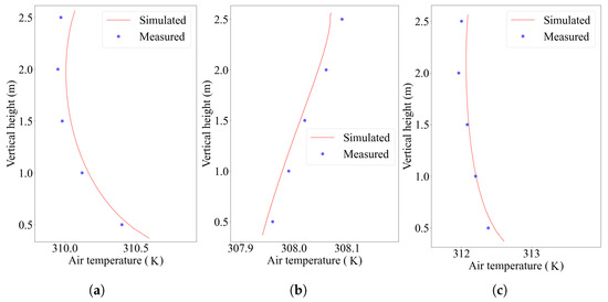
Figure 10.
Comparison between simulated and measured air temperatures at monitoring points: (a) point A, (b) point B, and (c) point C.
Figure 11 illustrates the vertical temperature profiles recorded at 0:00 for the three monitoring points highlighted in Figure 3. The highest temperatures in the floor domain are observed at the pipe region for all monitoring points. At midnight, without solar radiation effects, the temperature within the air domain is primarily influenced by the flow field and the temperature field in underfloor pipes. Compared with points B and C, there is an unheated area (near the south-facing window) in the zone where point A is located, resulting in noticeable differences in water supply temperature and air temperatures.
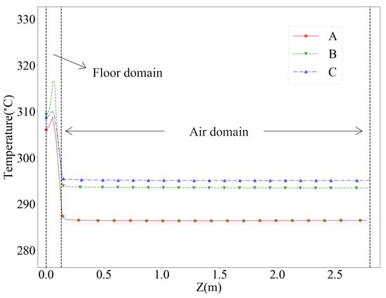
Figure 11.
Vertical temperature profiles at monitoring points at 0:00.
Figure 12 illustrates the vertical temperature profiles recorded at 12:00 for the monitoring points. At 12:00 a.m., A and B are exposed directly to solar radiation, leading to the highest temperature at the floor surface and significant temperature differences at different zones. Due to the uneven temperature distribution, the temperature at any monitoring point cannot represent the overall thermal comfort of the apartment, indicating the necessity for the sensor placement optimization.
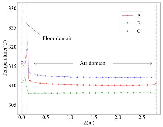
Figure 12.
Vertical temperature profiles at monitoring points at 12:00.
4.1.2. Radiant Floor Surface Temperature
Figure 13, Figure 14 and Figure 15 show the floor surface temperature contours at each moment over three days. Obviously, at 9:00, 12:00, and 15:00 each day, solar radiation passes through windows and acts on the floor surface, leading to the rise in local temperature. The figures show that solar radiation mainly affects zones 2, 5, and 6, with significantly higher floor surface temperature in the exposed areas, indicating an uneven temperature distribution across the entire radiant floor. The maximum temperature in the area directly exposed to the sun can reach 315 K, while the temperature in the shadow area is 290 K. As the Earth orbits the sun and rotates on its axis, the sunray’s direction and intensity vary over time, as well as the exposed area of the floor surface.
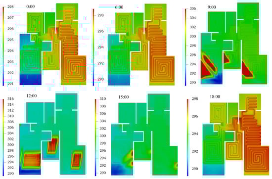
Figure 13.
Floor surface temperature contours for the first day (date: 1 November).
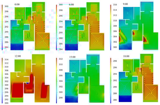
Figure 14.
Floor surface temperature contours for the second day (date: 12 December).
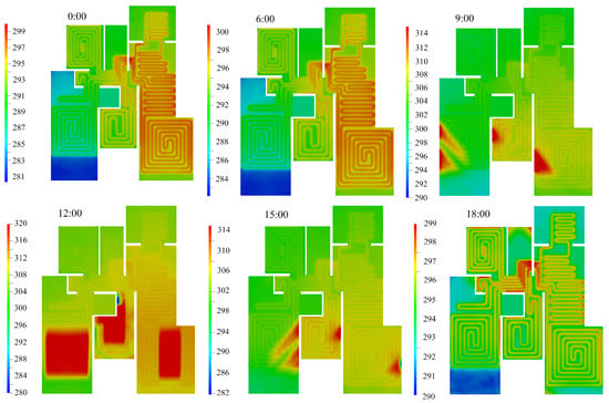
Figure 15.
Floor surface temperature contours for the third day (date: 24 January).
4.1.3. Zone Operative Temperature
Figure 16 shows a boxplot of the volume-averaged operative temperature of all zones for different times. Significant temperature differences can be observed between different zones, although all zones exhibit similar trends in temperature changes. The supply water temperature of the floor radiant heating system is adjusted according to the outdoor temperature, without taking into account the influence of solar radiation. As a result, all zones experience a noticeable temperature increase during periods of sunlight, even in shaded areas. The active control strategy increases the difficulty in the optimization of the sensor placement.
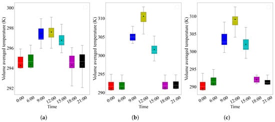
Figure 16.
Boxplot of volume-averaged operative temperature of all zones for different times: (a) 1 November, (b) 12 December, and (c) 24 January.
4.2. Mean and Standard Deviation of
The quantitative indicator reflects the appropriate sensor locations to a certain extent. However, for different stages of the heating season, the applicability and optimal positions of this indicator may vary. To obtain more accurate results, the averaged value of the quantized metrics at different stages was averaged, as well as the standard deviation value to reflect the stability of the temperature field.
Averaging over all scenarios, the mean values of for a 1.0 m plane are extracted. Figure 17 shows the contour maps of the mean , with gray areas indicating walls excluded from the numerical analysis. Areas where the mean values approach zero suggest that the local temperature closely approximates the volume-averaged operative temperature of the corresponding zone. For a specified zone, the lowest mean values within the entire dataset are always observed at its corresponding matching area. For example, the lowest mean values for zone 2 appear in zone 2. Therefore, if zone 2 is the only concern, the temperature sensor can be just placed within zone 2. The area where the mean value is closest to 0 indicates the optimal location for sensor placement. However, zones exposed to solar radiation or near windows have relatively high mean values and are not recommended for sensor placement, such as zone 5.
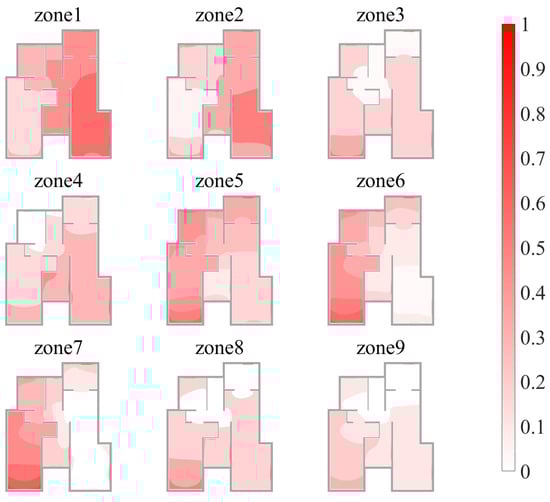
Figure 17.
Contours of the mean value of G Tavg for each zone at a 1.0 m plane.
To accurately capture the zone’s temperature characteristics across scenarios, relying solely on the mean value is inadequate and must be complemented by its variance. Figure 18 shows the contour maps of the standard deviation of for different zones. Locations with standard deviations close to 0 indicate that the local temperature can represent the volume-averaged operative temperature of the specified zone, similar to the mean value. Zones exposed to direct sunlight or near windows have relatively high standard deviation values for .
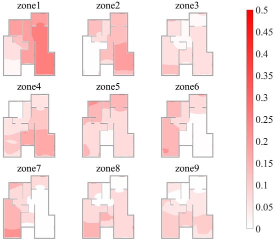
Figure 18.
Contours of standard deviation of G Tavg for each zone at a 1.0 m plane.
In order to find the region with low mean and standard deviation values of , scatter plots of these two values for a 1.0 m plane are plotted in Figure 19. As the mean value of increases, the distribution of the standard deviation becomes more dispersed, particularly in the region where the average is above 0.23. By cross-selecting the standard deviation and mean value datasets for zones 1 to 9 on the plane, a positive correlation emerges in the region with mean values of less than 0.23 and standard deviations of less than 0.13. Within this range, areas with lower average values typically have lower standard deviations, indicating that these regions experience smaller temperature fluctuations and more uniform temperature distribution.
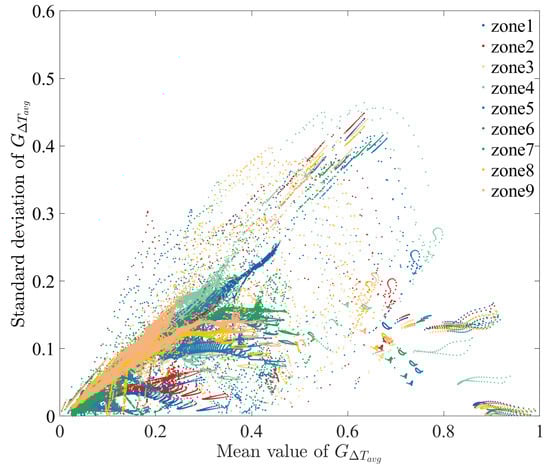
Figure 19.
Scatter plot of standard deviation versus mean value of at a 1.0 m plane.
Additionally, over 65% of the datasets on each plane fall within this range. The data within this region were extracted and subjected to linear fitting. The regression line in Figure 20 shows that the (coefficient of determination) for a 1.0 m plane is above 0.8. The corresponding contour maps and scatter plots for other selected planes can be found in the Supplementary Materials.
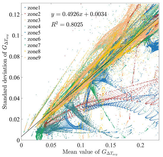
Figure 20.
Linear relationship between standard deviation and mean value of at a 1.0 m plane.
4.3. Optimal Temperature Sensor Locations
After analyzing the mean and standard deviation values of for all planes, the same procedure was repeated for all planes. A comparison of and the proportion of included data across different heights is shown in Figure 21.
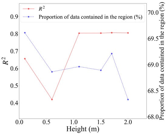
Figure 21.
and the proportion of included data across different heights.
The results reveal a poor fit for the linear regression model when applied to the 0.1 m and 0.6 m planes, with = 0.66 for a 0.1 m plane and = 0.42 for a 0.6 m plane. Therefore, these two planes are unsuitable for sensor placement and discarded in the subsequent analysis.
Based on above analysis, we summarized the conditions that sensor locations must meet: (1) the mean is less than 0.23, and (2) the standard deviation of is less than 0.13. The locations meeting these conditions for all planes are shown in Figure 22.
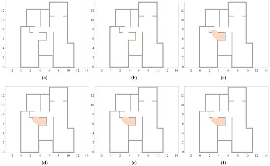
Figure 22.
Optimal sensor placement maps at different planes: (a) 0.1 m, (b) 0.6 m, (c) 1.0 m, (d) 1.5 m, (e) 1.7 m, and (f) 2.0 m.
For the planes at heights of 0.1 m and 0.6 m, the figures are nearly completely blank, indicating that there are no measurement points meeting the criteria at these heights. This means that the temperature distribution at these heights exhibits strong non-uniformity, with no stable measurement points available as candidates for sensor placement. For the planes above 1.0 m, the optimal sensor locations vary slightly across different planes. The optimal sensor placement should avoid areas with significant temperature fluctuations, such as near the floor, exterior walls, windows, and areas exposed to direct sunlight.
4.4. Validation of Determined Monitoring Point Locations
Figure 23 shows the root mean square error (RMSE) between the temperatures predicted by the above optimal sensor locations and the weighted average of the actual volume-averaged operative temperatures of all zones across scenarios. It is found that the RMSE values on 12 December was relatively high, reaching up to 0.35 °C, due to the large exposed area of solar radiation on the floor surface. At other times, the RMSE values remain below 0.3 °C. The RMSE results demonstrate that the selected sensor locations can effectively predict the true thermal comfort temperatures across the room’s active zones in the apartment, potentially reducing the potential error between actual and measured temperatures compared with a randomly placed sensor.
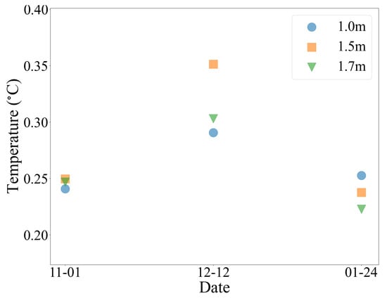
Figure 23.
Temperature prediction errors of the optimal sensor location across different levels.
5. Conclusions
In this paper, we propose a data-driven method for quantifying indoor temperature sensor locations in a multi-apartment building with radiant floor heating. The proposed method ensures that the selected temperature sensor locations can reflect the actual volume-averaged temperature of each zone under different boundary conditions.
A detailed CFD model consisting of eight domains (air, floor, and underfloor pipes) was established and applied under various outdoor temperatures, corresponding supply water temperatures, and solar radiation with ray tracing. The results indicate that there is a significant temperature difference on the floor surface across different areas, leading to differences in thermal comfort across zones, especially in the presence of solar radiation. The exposed area of solar radiation on the floor surface changes over time, with temperature differences reaching 25 K. This makes it difficult for randomly placed temperature sensors to predict accurate temperatures at corresponding locations.
The optimal sensor locations determined are defined as the positions that represent the overall thermal comfort of the apartment under various operating conditions. Under radiant floor heating, thermal comfort can be evaluated by the operative temperature, which depends on the outdoor temperature and solar radiation. In the heating season, throughout different dates of the year and various times of the day, the angle and intensity of solar radiation continuously change, causing fluctuations in indoor temperature distribution during daylight hours. As a result, the optimal measurement point that reflects the overall indoor thermal comfort also constantly shifts. Therefore, during the heating period, three typical days were selected, and within each day, seven time points were chosen to conduct multiple operating condition simulations.
A normalized metric was introduced to determine the optimal sensor location by cross-selecting the standard deviation and mean value datasets for zones 1 to 9 on a specified plane. Results show that sensors need to be placed on planes ranging from 1.0 m to 1.7 m, with specific locations visualized. Through RMSE analysis, it is found that the RMSE values between the predicted temperatures at the selected sensor locations and the actual temperatures are mostly less than 0.3 °C. This further validates the prediction accuracy of the selected temperature sensor locations.
This approach ensures that the simulation results can cover the impact of outdoor temperatures and solar radiation under various different operating conditions. For the apartment studied in this article, the selected operating conditions cover all possible scenarios throughout the heating season. Consequently, the optimal sensor locations obtained are equally applicable to all operating conditions during the heating season. However, for apartments with different building typologies, due to variations in room layout and orientation, the optimal sensor locations derived in this study have a limited reference value. For example, the sensor position should avoid direct sunlight and be kept away from the external enclosure. The specific optimal sensor locations still require repeating the methodology outlined in this study.
Room temperature monitoring is essential for both the regulation of the central heating system and personalized control for a single user. Recently, with the advancements in IoT and sensor technologies, the application of a remote room temperature collection system has become increasingly widespread. This study provides reliable recommendations for the placement of indoor temperature sensors.
Supplementary Materials
The following supporting information can be downloaded at: https://www.mdpi.com/article/10.3390/buildings15122026/s1, Figure S1–S5: Contours of mean value of for each zone at selected planes other than 1.0 m; Figure S6–S10: Contours of standard deviation of for each zone at selected planes other than 1.0 m; Figure S11–S15: Scatter plots of standard deviation versus mean value of at selected planes other than 1.0 m; Figure S16–S20: Linear relationship between standard deviation and mean value of at selected planes other than 1.0 m.
Author Contributions
Conceptualization, G.W. and S.L.; methodology, S.L.; software, G.W.; validation, S.L. and H.W.; formal analysis, S.L. and H.W.; investigation, S.L.; resources, H.W.; data curation, S.L.; writing—original draft preparation, G.W.; writing—review and editing, G.W.; visualization, S.L. and G.W.; supervision, G.W. and H.W.; project administration, G.W.; funding acquisition, G.W. All authors have read and agreed to the published version of the manuscript.
Funding
This research was funded by the National Key Research and Development Program of China through grant number 2021YFE0116200 and the Fundamental Research Program of the Education Department of Liaoning Province through grant numbers JYTZD2023166 and JYTMS20231594.
Data Availability Statement
The raw data supporting the conclusions of this article will be made available by the authors on request.
Conflicts of Interest
The authors declare no conflicts of interest.
Abbreviations
The following abbreviations are used in this manuscript:
| OSP | optimal sensor placement |
| CFD | computational fluid dynamics |
| RMSE | root mean square errors |
| HVAC | heating, ventilation, and air conditioning |
| DO | discrete ordinates |
| MRT | mean radiant temperature |
References
- Park, S.H.; Chung, W.J.; Yeo, M.S.; Kim, K.W. Evaluation of the thermal performance of a Thermally Activated Building System (TABS) according to the thermal load in a residential building. Energy Build. 2014, 73, 69–82. [Google Scholar] [CrossRef]
- Fabrizio, E.; Corgnati, S.P.; Causone, F.; Filippi, M. Numerical comparison between energy and comfort performances of radiant heating and cooling systems versus air systems. Sci. Technol. Built Environ. 2012, 18, 692–708. [Google Scholar] [CrossRef]
- Zou, C.; Li, B.; Wang, X.; Liu, S. Research on indoor dynamic temperature based on circulating water heating. Energy Rep. 2023, 10, 1091–1098. [Google Scholar] [CrossRef]
- Nicoletti, V.; Simone, Q.; Lorenzo, A.; Gara, F. Assessment of Different Optimal Sensor Placement Methods for Dynamic Monitoring of Civil Structures and Infrastructures. Struct. Infrastruct. Eng. 2024, 1–16. [Google Scholar] [CrossRef]
- Hosseini, H.; Taleai, M.; Zlatanova, S. NSGA-II Based Optimal Wi-Fi Access Point Placement for Indoor Positioning: A BIM-based RSS Prediction. Autom. Constr. 2023, 152, 104897. [Google Scholar] [CrossRef]
- Yan, Y.; Li, X.; Yang, L.; Tu, J. Evaluation of manikin simplification methods for CFD simulations in occupied indoor environments. Energy Build. 2016, 127, 611–626. [Google Scholar] [CrossRef]
- Bae, Y.; Bhattacharya, S.; Cui, B.; Lee, S.; Li, Y.; Zhang, L.; Kuruganti, T. Sensor impacts on building and HVAC controls: A critical review for building energy performance. Adv. Appl. Energy 2021, 4, 100068. [Google Scholar] [CrossRef]
- ASHRAE Standard 55-2004; Thermal Environmental Conditions for Human Occupancy. Technical report. ASHRAE: Atlanta, GA, USA, 2004.
- Bucarelli, N.; El-Gohary, N. Consensus-Based Clustering for Indoor Sensor Deployment and Indoor Condition Monitoring. Build. Environ. 2023, 244, 110550. [Google Scholar] [CrossRef]
- Yuan, M.; Geng, Y.; Lin, B.; Tang, H.; Yang, Y. Optimization of Indoor Temperature Sensor Deployment in Large Spaces for Multiple Building Operation Scenarios Using the Genetic Algorithm. J. Build. Eng. 2024, 96, 110446. [Google Scholar] [CrossRef]
- Rackes, A.; Ben-David, T.; Waring, M.S. Sensor Networks for Routine Indoor Air Quality Monitoring in Buildings: Impacts of Placement, Accuracy, and Number of Sensors. Sci. Technol. Built Environ. 2018, 24, 188–197. [Google Scholar] [CrossRef]
- Ren, C.; Cao, S.J. Implementation and visualization of artificial intelligent ventilation control system using fast prediction models and limited monitoring data. Sustain. Cities Soc. 2020, 52, 101860. [Google Scholar] [CrossRef]
- Yoganathan, D.; Kondepudi, S.; Kalluri, B.; Manthapuri, S. Optimal sensor placement strategy for office buildings using clustering algorithms. Energy Build. 2018, 158, 1206–1225. [Google Scholar] [CrossRef]
- Suryanarayana, G.; Arroyo, J.; Helsen, L.; Lago, J. A data driven method for optimal sensor placement in multi-zone buildings. Energy Build. 2021, 243, 110956. [Google Scholar] [CrossRef]
- Man, X.; Lu, Y.; Li, G.; Wang, Y.; Liu, J. A Study on the Stack Effect of a Super High-Rise Residential Building in a Severe Cold Region in China. Indoor Built Environ. 2020, 29, 255–269. [Google Scholar] [CrossRef]
- Lu, M.; Xu, G.; Yuan, J. Installation Principle and Calculation Model of the Representative Indoor Temperature-Monitoring Points in Large-Scale Buildings. Energies 2023, 16, 6376. [Google Scholar] [CrossRef]
- Cao, S.J.; Ding, J.; Ren, C. Sensor Deployment Strategy Using Cluster Analysis of Fuzzy C-Means Algorithm: Towards Online Control of Indoor Environment’s Safety and Health. Sustain. Cities Soc. 2020, 59, 102190. [Google Scholar] [CrossRef]
- Shao, X.; Wang, K.; Li, X. Rapid prediction of the transient effect of the initial contaminant condition using a limited number of sensors. Indoor Built Environ. 2019, 28, 322–334. [Google Scholar] [CrossRef]
- Barbaresi, A.; Torreggiani, D.; Benni, S.; Tassinari, P. Indoor Air Temperature Monitoring: A Method Lending Support to Management and Design Tested on a Wine-Aging Room. Build. Environ. 2015, 86, 203–210. [Google Scholar] [CrossRef]
- Zhu, H.C.; Yu, C.W.; Cao, S.J. Ventilation Online Monitoring and Control System from the Perspectives of Technology Application. Indoor Built Environ. 2020, 29, 587–602. [Google Scholar] [CrossRef]
- Huang, Y.; Gao, Z.; Zhang, H. Comparison of Common Machine Learning Algorithms Trained with Multi-Zone Models for Identifying the Location and Strength of Indoor Pollutant Sources. Indoor Built Environ. 2021, 30, 1142–1158. [Google Scholar] [CrossRef]
- Ren, J.; Cao, S.J. Incorporating Online Monitoring Data into Fast Prediction Models towards the Development of Artificial Intelligent Ventilation Systems. Sustain. Cities Soc. 2019, 47, 101498. [Google Scholar] [CrossRef]
- Kyriacou, A.; Michaelides, M.P.; Eliades, D.G.; Panayiotou, C.G.; Polycarpou, M.M. COMOB: A MATLAB Toolbox for Sensor Placement and Contaminant Event Monitoring in Multi-Zone Buildings. Build. Environ. 2019, 154, 348–361. [Google Scholar] [CrossRef]
- Rong, Q.; Yan, D.; Zhou, X.; Jiang, Y. Research on a dynamic simulation method of atrium thermal environment based on neural network. Build. Environ. 2012, 50, 214–220. [Google Scholar] [CrossRef]
- Liu, Y.; Mao, W.; Diaz-Elsayed, N. An investigation of the indoor environment and its influence on manufacturing applications via computational fluid dynamics simulation. Build. Environ. 2022, 219, 109161. [Google Scholar] [CrossRef]
- Chua, K.; Chou, S.; Yang, W.; Yan, J. Achieving better energy-efficient air conditioning – A review of technologies and strategies. Appl. Energy 2013, 104, 87–104. [Google Scholar] [CrossRef]
- Stavrakakis, G.; Zervas, P.; Sarimveis, H.; Markatos, N. Development of a computational tool to quantify architectural-design effects on thermal comfort in naturally ventilated rural houses. Build. Environ. 2010, 45, 65–80. [Google Scholar] [CrossRef]
- Zhou, H.; Soh, Y.C.; Wu, X. Integrated analysis of CFD data with K-means clustering algorithm and extreme learning machine for localized HVAC control. Appl. Therm. Eng. 2015, 76, 98–104. [Google Scholar] [CrossRef]
- Djatouti, Z.; Waeytens, J.; Chamoin, L.; Chatellier, P. Goal-oriented sensor placement and model updating strategies applied to a real building in the Sense-City equipment under controlled winter and heat wave scenarios. Energy Build. 2021, 231, 110486. [Google Scholar] [CrossRef]
- Tian, W.; Han, X.; Zuo, W.; Wang, Q.; Fu, Y.; Jin, M. An optimization platform based on coupled indoor environment and HVAC simulation and its application in optimal thermostat placement. Energy Build. 2019, 199, 342–351. [Google Scholar] [CrossRef]
- Du, Z.; Xu, P.; Jin, X.; Liu, Q. Temperature sensor placement optimization for VAV control using CFD–BES co-simulation strategy. Build. Environ. 2015, 85, 104–113. [Google Scholar] [CrossRef]
- Li, K.; Wen, Z.; Xue, W.; Wang, Z. Fast reconstruction of indoor temperature field for large-space building based on limited sensors: An experimental study. Energy Build. 2023, 298, 113493. [Google Scholar] [CrossRef]
- Jiang, C.; Soh, Y.C.; Li, H. Two-stage indoor physical field reconstruction from sparse sensor observations. Energy Build. 2017, 151, 548–563. [Google Scholar] [CrossRef]
- Chen, C.; Gorlé, C. Optimal temperature sensor placement in buildings with buoyancy-driven natural ventilation using computational fluid dynamics and uncertainty quantification. Build. Environ. 2022, 207, 108496. [Google Scholar] [CrossRef]
- Yang, E. Research on control property of low-temperature floor radiant heating system. Open Constr. Build. Technol. J. 2015, 9, 311–315. [Google Scholar] [CrossRef][Green Version]
- Chen, Q.; Li, N.; Feng, W. Model predictive control optimization for rapid response and energy efficiency based on the state-space model of a radiant floor heating system. Energy Build. 2021, 238, 110832. [Google Scholar] [CrossRef]
- Wang, X.; Zhang, W.; Li, Q.; Wei, Z.; Lei, W.; Zhang, L. An Analytical Method to Estimate Temperature Distribution of Typical Radiant Floor Cooling Systems with Internal Heat Radiation. Energy Explor. Exploit. 2021, 39, 1283–1305. [Google Scholar] [CrossRef]
- Ling, J.; Li, Q.; Xing, J. The Influence of Apartment Location on Household Space Heating Consumption in Multi-Apartment Buildings. Energy Build. 2015, 103, 185–197. [Google Scholar] [CrossRef]
- Michnikowski, P. Allocation of Heating Costs with Consideration to Energy Transfer from Adjacent Apartments. Energy Build. 2017, 139, 224–231. [Google Scholar] [CrossRef]
- Zhang, Y.; Zhang, M.; Gao, F.; Li, J. Experimental Study on Internal Heat Transfer among Adjacent Rooms for Building Energy Efficiency with Housing Vacancy Consideration. Case Stud. Therm. Eng. 2024, 62, 105188. [Google Scholar] [CrossRef]
- Rohdin, P.; Moshfegh, B. Numerical Predictions of Indoor Climate in Large Industrial Premises. A Comparison between Different k–ε Models Supported by Field Measurements. Build. Environ. 2007, 42, 3872–3882. [Google Scholar] [CrossRef]
- Rohdin, P.; Moshfegh, B. Numerical Modeling of Indoor Climate and Air Quality in Industrial Environments-A Comparison between Different Turbulence Models and Supply Systems Supported by Field Measurements. Build. Environ. 2011, 46, 2011. [Google Scholar] [CrossRef]
- Zhang, Z.; Zhang, W.; Zhai, Z.J.; Chen, Q.Y. Evaluation of Various Turbulence Models in Predicting Airflow and Turbulence in Enclosed Environments by CFD: Part 2—Comparison with Experimental Data from Literature. HVAC&R Res. 2007, 13, 871–886. [Google Scholar] [CrossRef]
- Zhai, Z.J.; Zhang, Z.; Zhang, W.; Chen, Q.Y. Evaluation of Various Turbulence Models in Predicting Airflow and Turbulence in Enclosed Environments by CFD: Part 1—Summary of Prevalent Turbulence Models. HVAC&R Res. 2007, 13, 853–870. [Google Scholar] [CrossRef]
- Elmaghraby, H.A.; Chiang, Y.W.; Aliabadi, A.A. Ventilation Strategies and Air Quality Management in Passenger Aircraft Cabins: A Review of Experimental Approaches and Numerical Simulations. Sci. Technol. Built Environ. 2018, 24, 160–175. [Google Scholar] [CrossRef]
- Elmaghraby, H.A.; Chiang, Y.W.; Aliabadi, A.A. Are Aircraft Acceleration-Induced Body Forces Effective on Contaminant Dispersion in Passenger Aircraft Cabins? Sci. Technol. Built Environ. 2019, 25, 858–872. [Google Scholar] [CrossRef]
- Hang, J.; Buccolieri, R.; Yang, X.; Yang, H.; Quarta, F.; Wang, B. Impact of Indoor-Outdoor Temperature Differences on Dispersion of Gaseous Pollutant and Particles in Idealized Street Canyons with and without Viaduct Settings. Build. Simul. 2019, 12, 285–297. [Google Scholar] [CrossRef]
- Allegrini, J.; Dorer, V.; Carmeliet, J. Buoyant Flows in Street Canyons: Validation of CFD Simulations with Wind Tunnel Measurements. Build. Environ. 2014, 72, 63–74. [Google Scholar] [CrossRef]
- Walker, C.; Tan, G.; Glicksman, L. Reduced-Scale Building Model and Numerical Investigations to Buoyancy-Driven Natural Ventilation. Energy Build. 2011, 43, 2404–2413. [Google Scholar] [CrossRef]
- Ji, Y.; Cook, M.J.; Hanby, V. CFD Modelling of Natural Displacement Ventilation in an Enclosure Connected to an Atrium. Build. Environ. 2007, 42, 1158–1172. [Google Scholar] [CrossRef]
- Ji, Y.; Cook, M. Numerical Studies of Displacement Natural Ventilation in Multi-Storey Buildings Connected to an Atrium. Build. Serv. Eng. Res. Technol. 2007, 28, 207–222. [Google Scholar] [CrossRef]
- Tabarki, M.; Mabrouk, S.B. The Coupling in Transient Regime between the Modelings of Thermal and Mass Transfers inside a Heated Room and Its Radiator. Heat Mass Transf. 2012, 48, 1889–1901. [Google Scholar] [CrossRef]
- Chai, J.; Fan, J. Advanced thermal regulating materials and systems for energy saving and thermal comfort in buildings. Mater. Today Energy 2022, 24, 100925. [Google Scholar] [CrossRef]
Disclaimer/Publisher’s Note: The statements, opinions and data contained in all publications are solely those of the individual author(s) and contributor(s) and not of MDPI and/or the editor(s). MDPI and/or the editor(s) disclaim responsibility for any injury to people or property resulting from any ideas, methods, instructions or products referred to in the content. |
© 2025 by the authors. Licensee MDPI, Basel, Switzerland. This article is an open access article distributed under the terms and conditions of the Creative Commons Attribution (CC BY) license (https://creativecommons.org/licenses/by/4.0/).