The Heat Exchange Coefficient of the Cooling Tube Under the Influence of the Tube Material and Cooling Water Parameters

Abstract

The traditional finite element method deals with the temperature field around the cooling tube due to the computational efficiency problems caused by grid division and the uncertainty of the convective heat transfer coefficient, resulting in inaccurate calculation results around the cooling tube. We conducted experiments to study the thermal stress and temperature gradient caused by various factors such as different materials of cooling pipes, pipe diameters, cooling water temperatures, and flow rates. The results showed that aluminum alloy pipes had the highest cooling efficiency but also produced a large temperature gradient. Pipe diameter had the most significant impact on cooling efficiency. Additionally, it is recommended that the cooling water flow velocity is not less than 0.6 m/s to achieve the best efficiency for the cooling pipe of any pipe diameter. The influence range of the cooling pipe on concrete could vary with pipe material, flow rate, and ambient factors. Our experimental results were compared with other heat transfer formulas (the Dittus–Boelter formula and the Yang Joo-Kyoung formula). According to the measured results, the formula is modified). The modified formula can estimate the heat transfer coefficient more accurately according to the flow rate and pipeline characteristics. Finally, the applicability of the formula is further verified by comparing the concrete on the bottom plate of a dam. The proposed heat transfer prediction model can estimate the heat transfer coefficient according to the flow rate and pipeline characteristics, The accuracy of the convection coefficient under different working conditions is improved by 10–25%. It is convenient to predict concrete temperature in practical engineering.

1. Introduction

Previous studies have primarily relied on theoretical derivations and finite element simulations to analyze the thermal behavior of cooling pipes in mass concrete. While these approaches provide valuable insights, they often lack experimental validation under controlled conditions. For example, Liu et al. [1] proposed a heat-flow coupled model (HFCM) to simulate temperature distribution, but the model’s accuracy was limited by the absence of experimental data on the combined effects of pipe material and cooling water parameters. Similarly, Tasri et al. [2,3,4] conducted numerical studies on the impact of cooling pipe materials and water temperature but did not account for the influence of pipe diameter and flow rate variations.

In mass concrete structures, a significant amount of heat is rapidly generated and concentrated within the concrete due to the exothermic hydration of cement. This leads to a rapid increase in temperature, with a noticeable temperature difference from internal to external. The temperature inside the concrete can rise by 40–50 °C, reaching a maximum temperature of 70–80 °C [5]. Due to its low heat conductivity, concrete undergoes a slow natural cooling process. As a consequence, it undergoes tension stress and becomes extremely prone to temperature-induced cracking when the tensile stress it is exposed to exceeds its ultimate tensile strength [6,7,8]. Pipe cooling methods are widely employed to decrease hydration heat and manage cracking. However, extreme temperature differences within concrete near cooling pipes can potentially cause cracking [9]. The heat transfer between the pipe and the concrete depends on factors such as pipe diameter, flow rate, material, arrangement form, and water temperature [10,11], and it is important to consider the convective heat transfer coefficient in order to more accurately control concrete cracking. Liu [12] utilized a heat-flow coupling approach to analyze the pipe cooling system in mass concrete structures, focusing on factors such as pipe arrangement, cooling water velocity, inlet temperature, water temperature increase along the flow, and thermal performance of the cooling pipes. Joo Kyoung [13] created a model to predict the heat transfer coefficient of cooling water. This model takes into account variables such as the flow rate of the cooling water, diameter of the pipe, thickness of the wall, and material of the pipe. Peng [14] studied the cooling effect and local temperature gradient under different water flow and water temperature, and put forward relevant engineering suggestions.

During the thermal assessment of concrete with cooling pipes, it is essential to generate a highly refined and uniform mesh around the pipe axis for accurate temperature distribution analysis. This presents challenges in mesh generation, especially in three-dimensional scenarios [15,16]. To address the complexity of mesh refinement in traditional FEMs, Zuo [17] introduced an enhanced finite element approach (XFEM) to effectively analyze the thermal behavior of pipelines using a less detailed mesh, while still ensuring precision and dependability. Yudong [18] also presented a reasonable theoretical expression and effective numerical implementation of concrete hydration temperature evolution based on Fourier’s law. However, the actual temperature field in a project is influenced by various external factors. Nguyen [19] uses numerical methods and finite element simulations to analyze the effects of cement content, initial concrete temperature, and construction techniques on temperature distribution. The developed nomogram allows for quick determination of maximum temperatures, aiding in the design and construction of mass concrete structures. Seyednavid [20] presents a detailed methodology for predicting the early-age thermal behavior of mass concrete containing supplementary cementitious materials (SCMs) using ANSYS finite element software. Mansour [21] presents a practical 3D finite difference model (3D-FDM) developed using MS-Excel to predict the thermal behavior of mass concrete elements, specifically a bridge pile cap. The model accounts for heat transfer, hydration heat, and environmental conditions, and its results are validated against on-site temperature measurements recorded using thermocouples.

While previous studies have extensively investigated the effects of cooling pipe materials, diameters, and cooling water parameters on temperature control in mass concrete, there remain gaps in understanding the combined influence of these factors on the convective heat transfer coefficient. Most existing research focuses on individual parameters, such as pipe material or flow rate, but fails to provide a comprehensive model that integrates multiple variables to accurately predict heat transfer efficiency. Or the lack of applicability, can only be more in line with specific scenarios. This study aims to address this gap by systematically analyzing the combined effects of pipe material, diameter, cooling water temperature, and flow rate on the heat transfer coefficient, and proposing a modified heat transfer prediction model that can be applied to real-world engineering scenarios. The experimental device we designed can obtain the heat exchange coefficient through the change in water temperature outside the tube wall, and the water tank allows multiple experiments under controlled conditions, which significantly improves the experimental efficiency.

2. Experimental Investigation

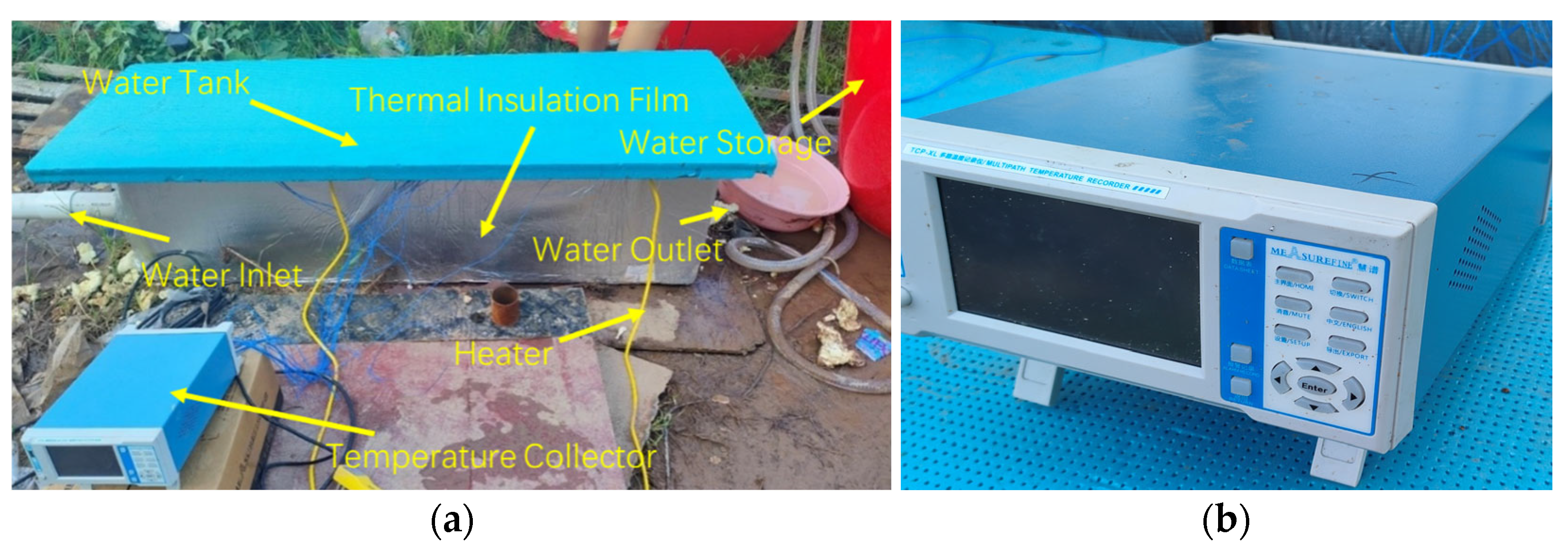
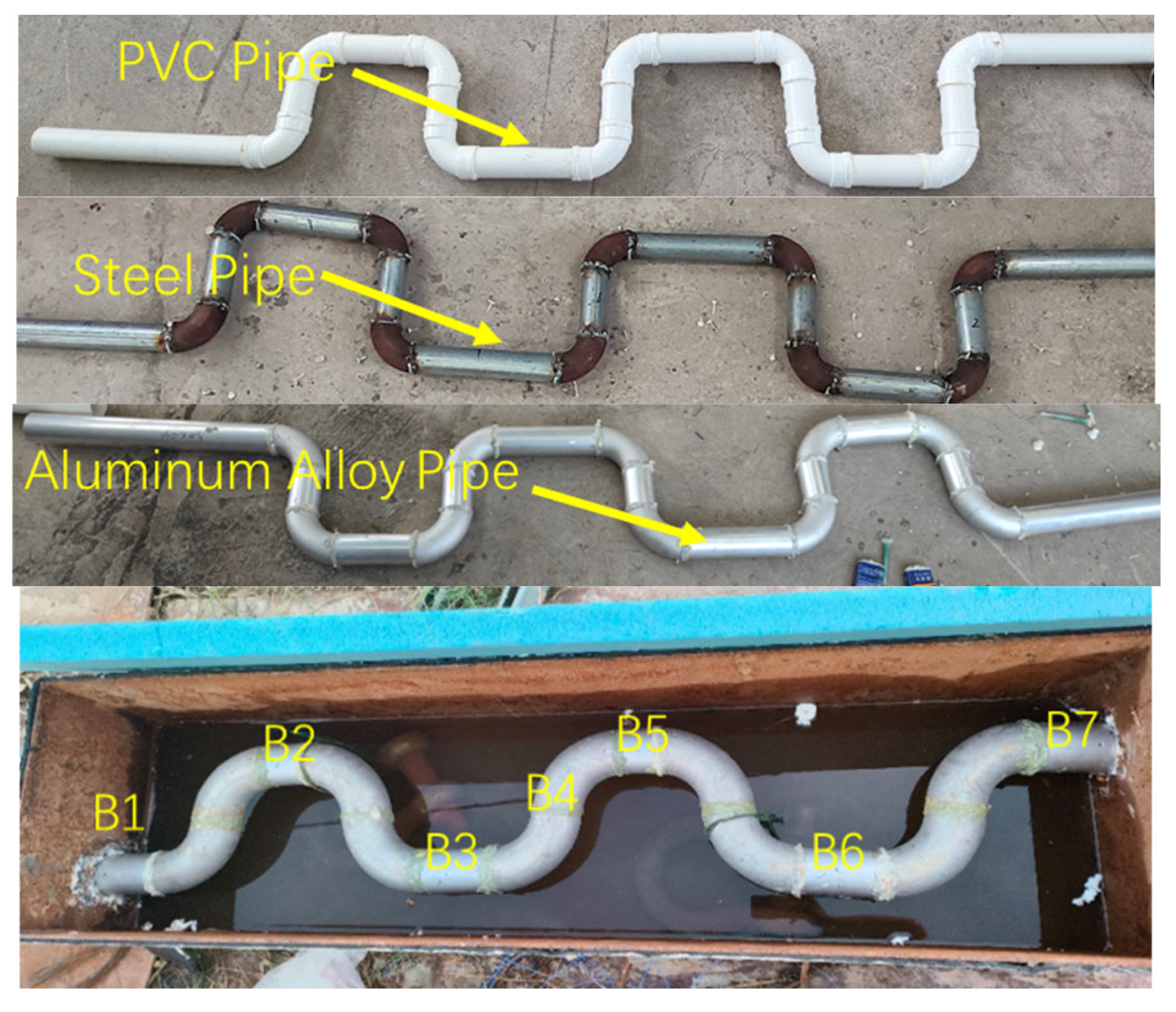
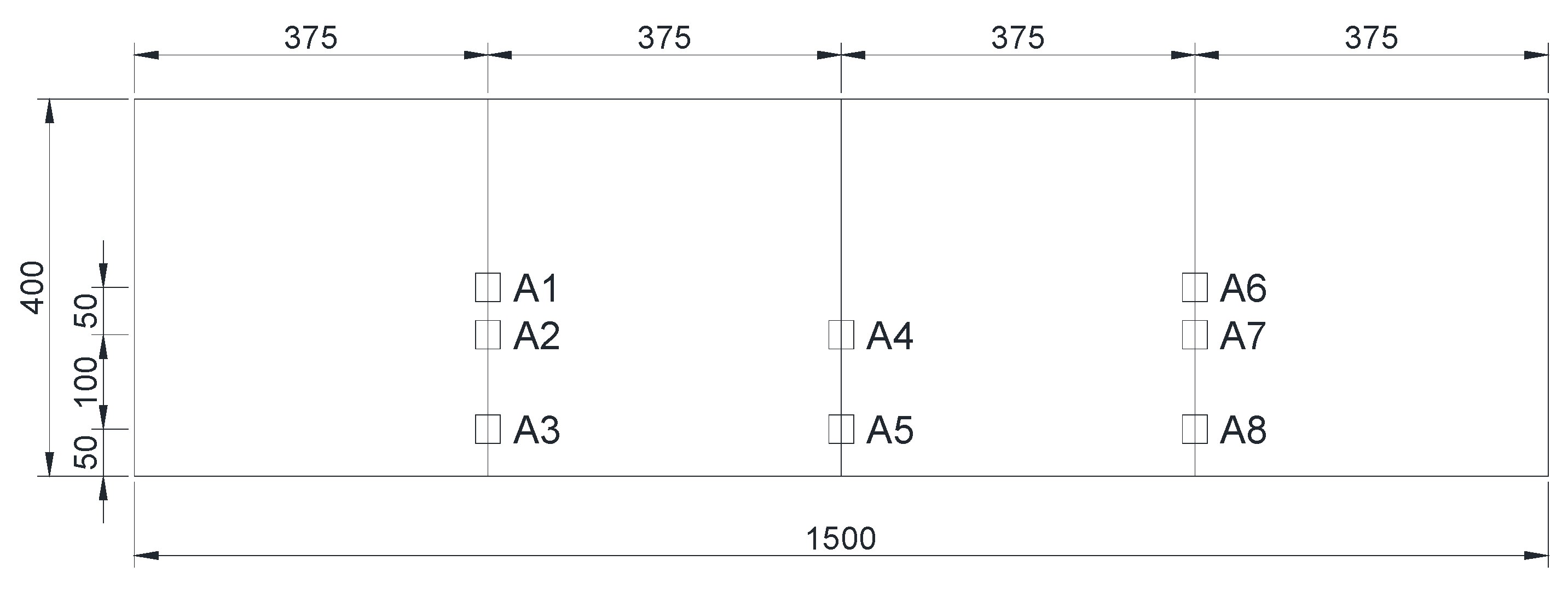
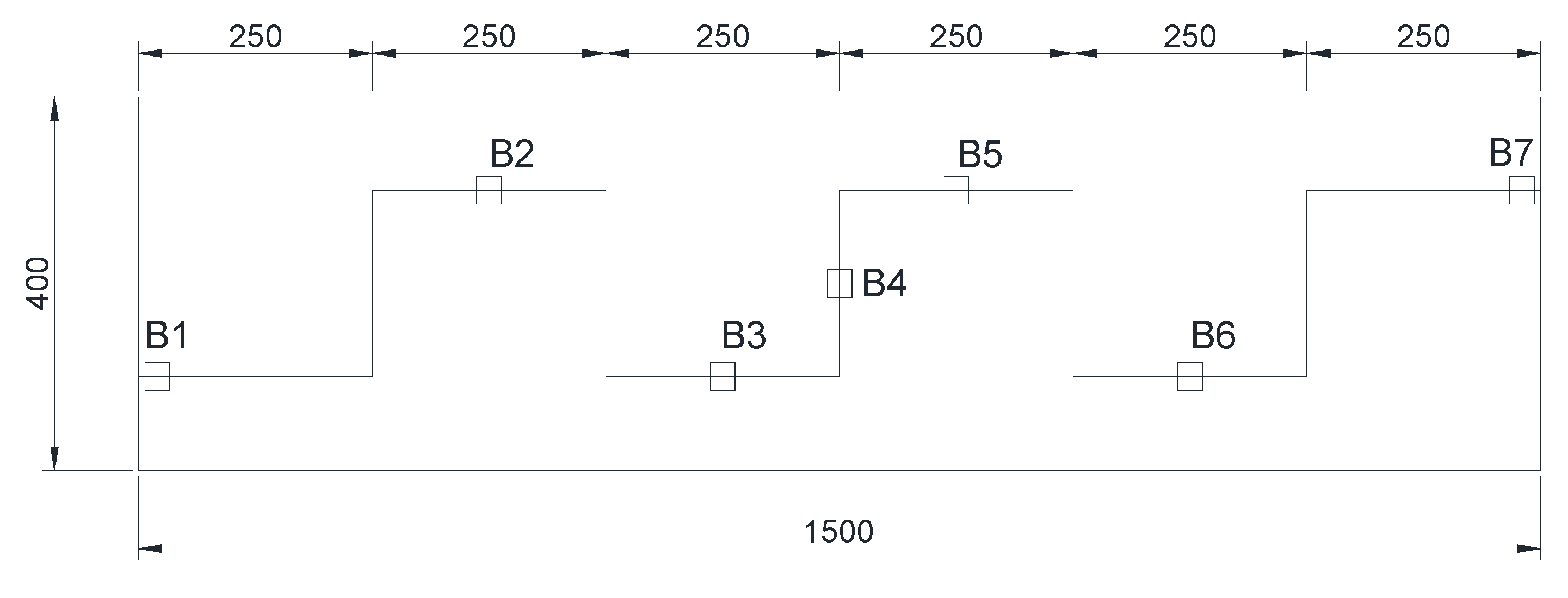
2.1. The Test Scheme

Cooling pipes are frequently employed in large concrete constructions to reduce the heat generated during hydration and control the formation of cracks. As a result, it is essential to accurately forecast the convective heat transfer coefficient, which signifies the transfer of heat between the fluid inside the pipe and the concrete. The main factors affecting this coefficient include pipe diameter, flow velocity, pipe material, arrangement form, and temperature of the cooling water. Accordingly, the pipe diameter, flow rate, pipe material, arrangement form and cooling water temperature are selected as the experimental parameters, the experimental device is designed for water cooling, the temperature changes at different locations are obtained through the deployment of temperature sensors, and the temperature changes under different influencing factors are analyzed in combination with the experimental results of the developed device.

The water tank is designed with a water circulation system and a measurement system, measuring 1.5 m × 0.4 m × 0.4 m in dimensions. The pump is linked to the cooling pipe inlet, drawing water from the bucket and controlling the flow rate. The initial temperature of the water tank is 60 °C, and the initial temperatures of the circulating water are 20 °C and 30 °C. An insulation film is applied externally to replicate adiabatic heat loss conditions and minimize heat loss to the surrounding environment. The field equipment layout and temperature acquisition instrument are shown in Figure 1.

The cooling pipe was installed in a water tank to simulate the heat exchange process between the pipe and the surrounding medium. Water was chosen as the medium for several reasons.

(1) Repeatability and Efficiency: Conducting experiments with concrete would require preparing new specimens for each test, which is time-consuming and resource intensive. The water tank setup allows for multiple experiments under controlled conditions, significantly improving experimental efficiency.

(2) Accuracy of Hydration Heat Simulation: Small concrete specimens may not accurately represent the hydration heat of mass concrete due to scale effects. The water tank provides a more controlled environment to study the heat exchange behavior, ensuring reliable and repeatable results.

(3) Temperature Regulation: Water allows for precise and rapid temperature adjustments, enabling us to study the effects of different cooling water temperatures and flow rates more effectively.

This experiment used steel pipes, PVC pipes, and aluminum pipes with three different pipe diameters, 32 mm, 42 mm, and 52 mm. In actual engineering cooling pipes, a serpentine arrangement was used, as illustrated in Figure 2.

The heat transfer process of the designed device consists of three parts.

(1) Convection between the medium outside the pipe and the outer surface of the pipe.

(2) Conduction through the pipe

(3) Convection occurs between the inner surface of the pipe and the cooling water of the pipe. In this study, the convective heat transfer coefficient is related to the third step in the process.

Using a TCP-32XL temperature inspector to measure the temperature, the temperature sensor sensitivity was 0.02 °C, the accuracy was ±0.1 °C, the temperature range was −20~150 °C, which can ensure the accuracy of the data in the experiment process. Before the equipment is used, the equipment manufacturer has carried out temperature calibration for TCP-32XL. Before the experiment, we used a thermometer (±0.1 °C) to test the accuracy of the temperature sensor and found that the temperature of the two was basically the same. The temperature measurement points included the following:

A.

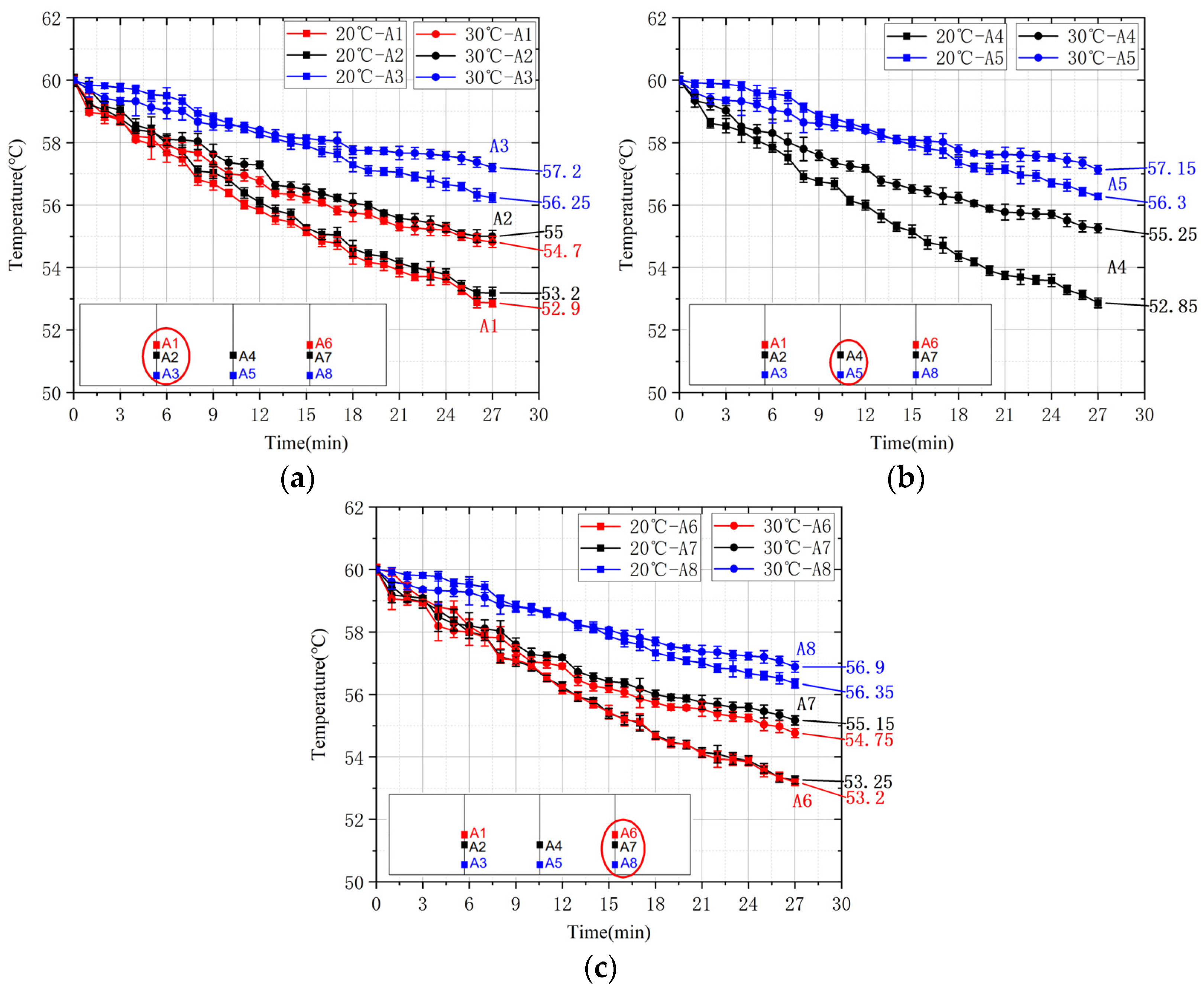
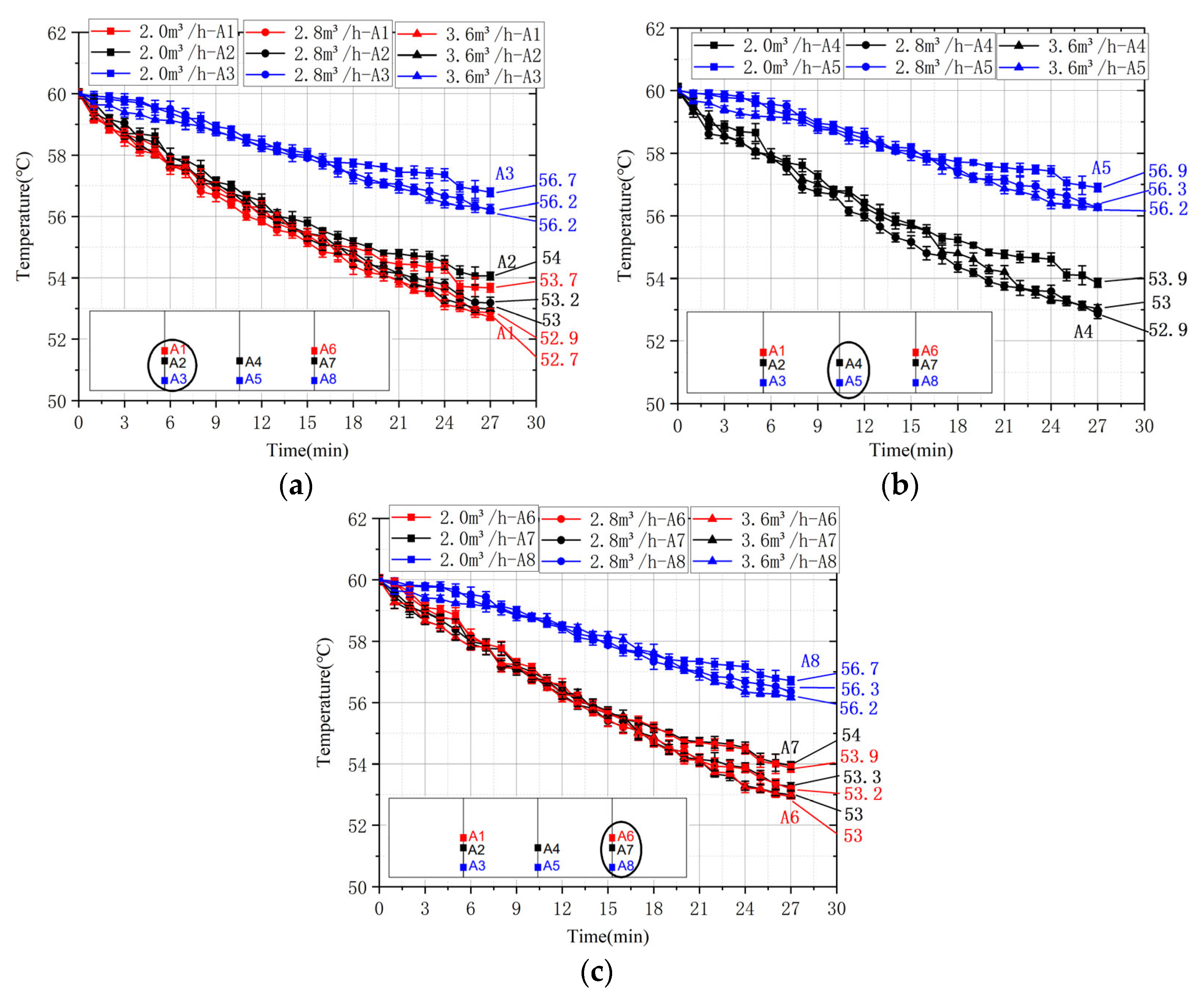
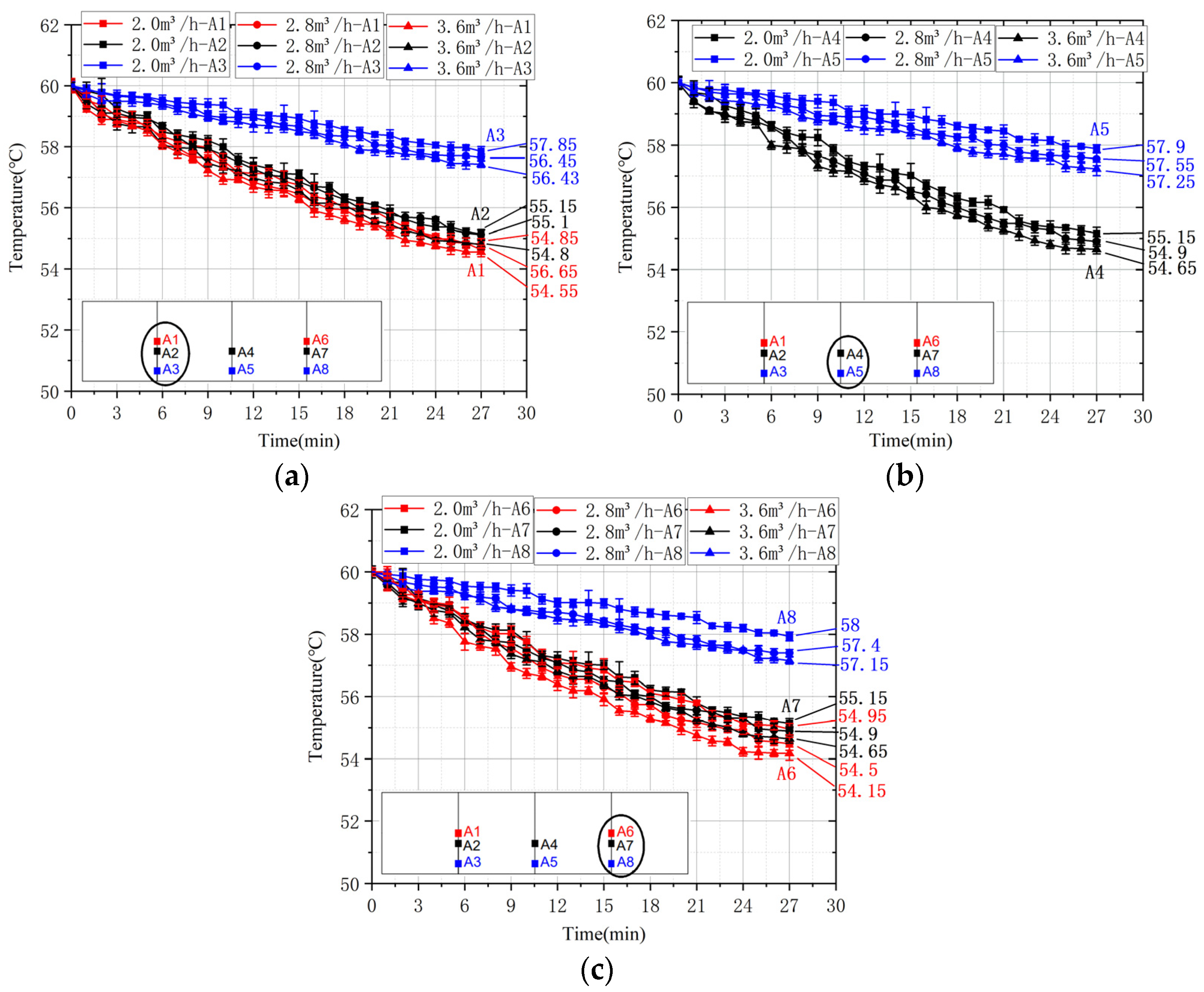
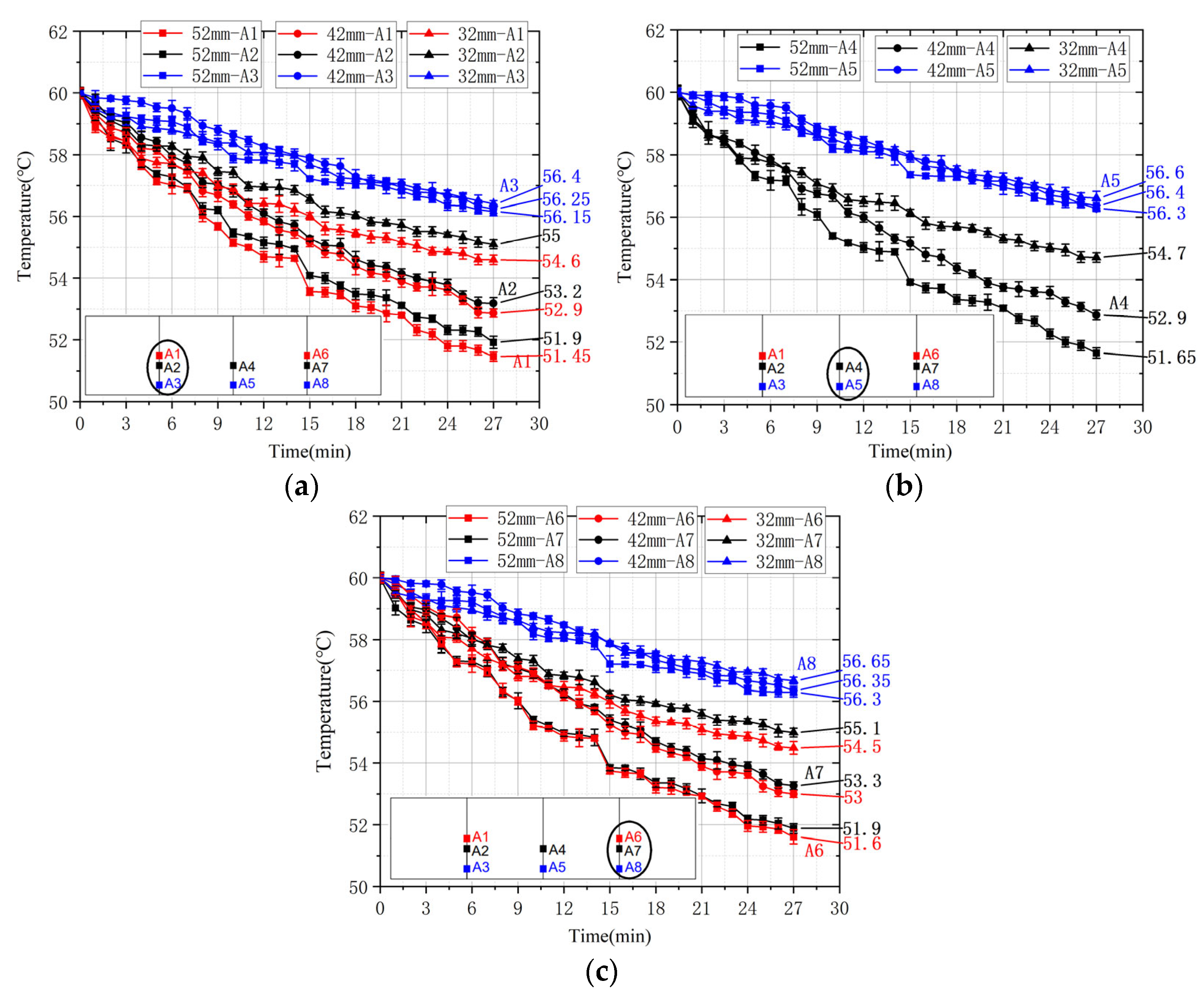
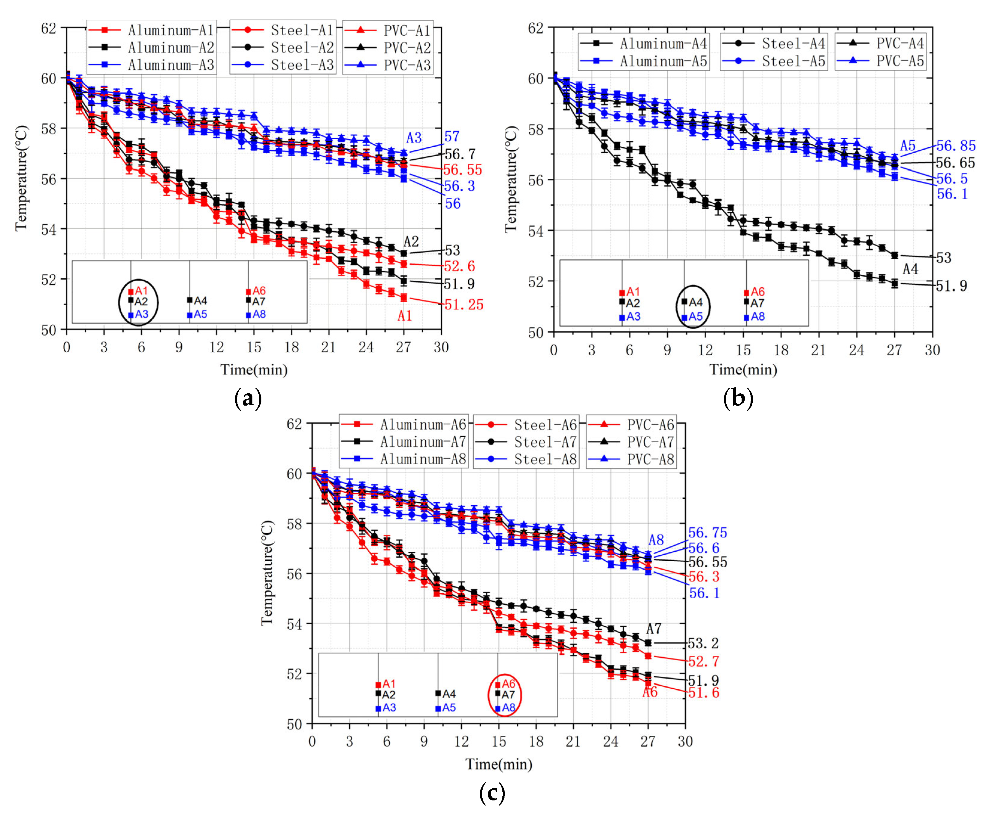
The tank water temperature is monitored at different points, such as near the cooling pipe inlet and outlet, and also at the middle of the outer wall of the pipe. The measurements are also taken at three different heights within the tank: the first layer (A1, A6) affixed to the cooling pipe, the second layer (A2, A4, A7) from the pipe 5 cm, and the third layer (A3, A5, A8) from the pipe 15 cm, as shown in Figure 3.

B.

Temperature changes in the water tank cooling tube temperature measurement points set to the center of each section of the tube to arrange a measurement point, the entrance and the exit of the layout of a measurement point, for a total of seven measurement points in the tube layout (B1~B7) in Figure 4.

2.2. Thermodynamic Properties of the Cooling Pipe

The effects of three commonly used cooling pipe materials on the temperature were investigated in this study. The materials for the pipes included steel, PVC, and aluminum alloy, and

Table 1. Thermal and mechanical properties of the cooling pipes.

	PVC	Steel	Aluminum Alloy
Thermal conductivity [KJ/m·h·°C)]	0.576	198	576
Specific heat [kJ/(kg °C)]	1.26	0.46	0.85
Density [kg/m3]	1600	7800	2680
Coefficient thermal expansion [10−6/°C]	70	11	23
Young’s modulus [GPa]	4.1	215	72
Poisson’s ratio [−]	0.4	0.3	0.3

displays the thermal properties of these three materials. The thermodynamic properties of the cooling pipes, including thermal conductivity, specific heat, density, coefficient of thermal expansion, Young’s modulus, and Poisson’s ratio, were sourced from material datasheets provided by the manufacturers and reference.

2.3. Experimental Parameters

Due to the different cooling pipe materials, pipe diameters, thermal conductivities, and cooling water parameters, tests of the thermal performance of different cooling pipe materials and cooling water parameters were performed.

Steel pipes, PVC pipes and aluminum alloy pipes are used as the cooling pipe materials, and each cooling pipe has a diameter of 32 mm, 42 mm, and 52 mm, of which the thickness of the pipe wall is 2 mm. Using different water flow rates and different water temperatures, an adiabatic water tank was cooled for 30 min, and the cooling changes in the water tank were monitored. The specific experimental parameters are detailed in

Table 2. Experimental parameters.

Diameter	Material	Temperature	Flow Rate
32 mm	Steel	20 °C	2.0 m3/h	2.8 m3/h	3.6 m3/h
		30 °C	2.0 m3/h	2.8 m3/h	3.6 m3/h
	Aluminum	20 °C	2.0 m3/h	2.8 m3/h	3.6 m3/h
		30 °C	2.0 m3/h	2.8 m3/h	3.6 m3/h
42 mm	Steel	20 °C	2.0 m3/h	2.8 m3/h	3.6 m3/h
		30 °C	2.0 m3/h	2.8 m3/h	3.6 m3/h
	Aluminum	20 °C	2.0 m3/h	2.8 m3/h	3.6 m3/h
		30 °C	2.0 m3/h	2.8 m3/h	3.6 m3/h
52 mm	PVC	20 °C	2.0 m3/h	2.8 m3/h	3.6 m3/h
		30 °C	2.0 m3/h	2.8 m3/h	3.6 m3/h
	Steel	20 °C	2.0 m3/h	2.8 m3/h	3.6 m3/h
		30 °C	2.0 m3/h	2.8 m3/h	3.6 m3/h
	Aluminum	20 °C	2.0 m3/h	2.8 m3/h	3.6 m3/h
		30 °C	2.0 m3/h	2.8 m3/h	3.6 m3/h

.

3. Test Results and Discussion

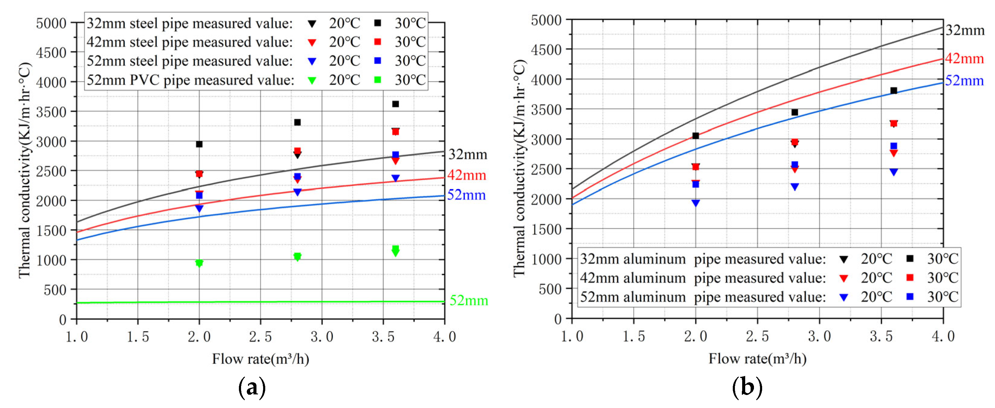
3.1. Effect of Water Temperature on Cooling

When the cooling water temperature is reduced from 30 °C to 20 °C, the temperature near the cooling tube decreases significantly after a period of water cooling as shown in Figure 5. The reduction in temperature is more pronounced in the region close to the cooling tube, while the effect of cooling water temperature on the final temperature diminishes with distance from the tube. The temperature differences at measurement points A3, A5, and A8 (15 cm from the cooling tube) were 0.6–0.9 °C, while at points A2, A4, and A7 (5 cm from the cooling tube), the differences were 1.8–2.4 °C. At points A1 and A6 (attached to the cooling tube wall), the temperature differences were 1.5–1.8 °C. Beyond 15 cm from the cooling tube, the change in cooling water temperature has minimal impact on the final temperature.

3.2. Effect of Water Flow Rate on Cooling

As shown in Figure 6, increasing the flow rate of the cooling water leads to a decrease in temperature around the cooling tube. However, beyond a certain flow rate, the temperature stabilizes, and further increases in flow rate have a diminishing effect on cooling efficiency. Specifically, when the flow rate was increased from 2.0 m³/h to 2.8 m³/h, the final temperatures at measurement points A3, A5, and A8 (15 cm from the cooling tube) decreased by 0.5 °C, while at points A2, A4, and A7 (5 cm from the cooling tube), the temperatures decreased by 0.9 °C. At points A1 and A6 (attached to the cooling tube wall), the temperatures decreased by 0.8 °C. When the flow rate was further increased from 2.8 m³/h to 3.6 m³/h, the temperature changes at all measurement points (A1–A8) were within a range of only 0.1 °C, indicating that the cooling efficiency stabilizes beyond a certain flow rate.

The stabilization of cooling efficiency beyond a flow rate of 2.8 m³/h can be attributed to the limitations imposed by the heat transfer dynamics between the cooling water and the water tank. At lower flow rates, the cooling water has sufficient time to absorb heat from water tank, resulting in a significant temperature drop. However, as the flow rate increases beyond a certain threshold, the cooling water passes through the pipe too quickly to fully absorb the heat, leading to diminishing returns in cooling efficiency. This phenomenon is further influenced by the pipe diameter, as larger diameters allow for greater heat exchange due to the increased surface area. Therefore, while higher flow rates can enhance cooling efficiency up to a point, the optimal flow rate must be carefully selected based on the pipe diameter and the specific cooling requirements of the project to avoid unnecessary energy consumption and operational costs.

Figure 6 shows the temperature variations at different flow rates when the pipe diameter is 42 mm. The results indicate that when the flow rate increases from 2.0 m³/h to 2.8 m³/h, the temperature change around the pipe diameter is relatively significant; however, when the flow rate further increases to 3.6 m³/h, the impact of the flow rate increase on the cooling effect becomes less obvious. Therefore, the critical flow rate for a pipe diameter of 42 mm is approximately 2.8 m³/h, corresponding to an optimal flow velocity of about 0.6 m/s. To further verify the limiting effect of pipe diameter on flow rate, water experiments were also conducted on 32 mm and 52 mm pipe diameters in Section 3.2 (commonly used pipe diameters in engineering include 32 mm, 42 mm and 52 mm). Figure 7 shows the temperature changes at different flow rates under a 32 mm pipe diameter. From a flow rate of 2.0 m³/h, the impact of further increasing the flow rate on the cooling effect is already very small. This indicates that the flow rate threshold for a 32 mm pipe diameter should be less than 2.0 m³/h, and the corresponding optimal flow velocity should be less than 0.7 m/s. Figure 8 shows the temperature changes at different flow rates under a 52 mm pipe diameter. We found that when the flow rate increased from 2.0 m³/h to 2.8 m³/h and then further to 3.6 m³/h, the temperature changes around the pipe diameter were relatively significant, and the flow rate had not yet reached the threshold. This indicates that the flow rate threshold for a 52 mm pipe diameter should be greater than 3.6 m³/h, and the corresponding optimal flow velocity should be greater than 0.5 m/s. The above research indicates that there is a critical threshold between flow rate and pipe diameter. Based on the analysis results mentioned above, we have selected 0.6 m/s as the optimal flow velocity applicable to all pipe diameters.

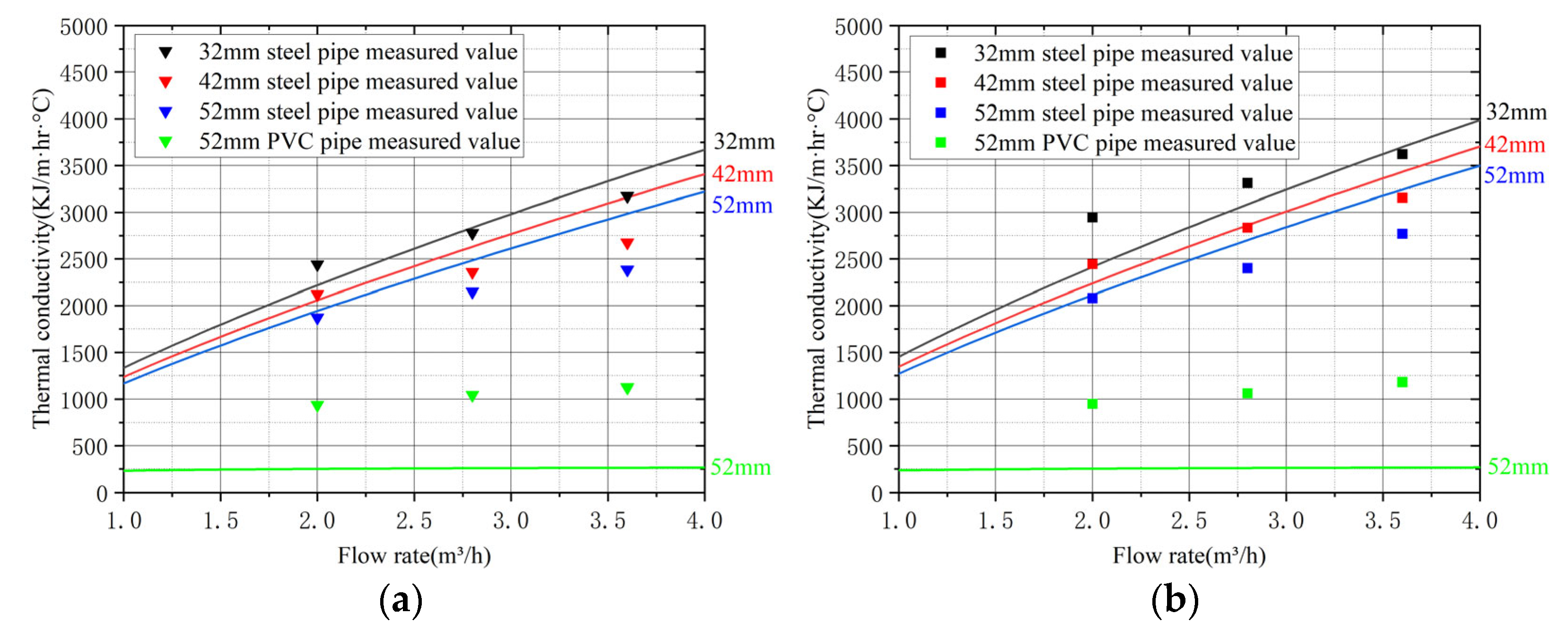
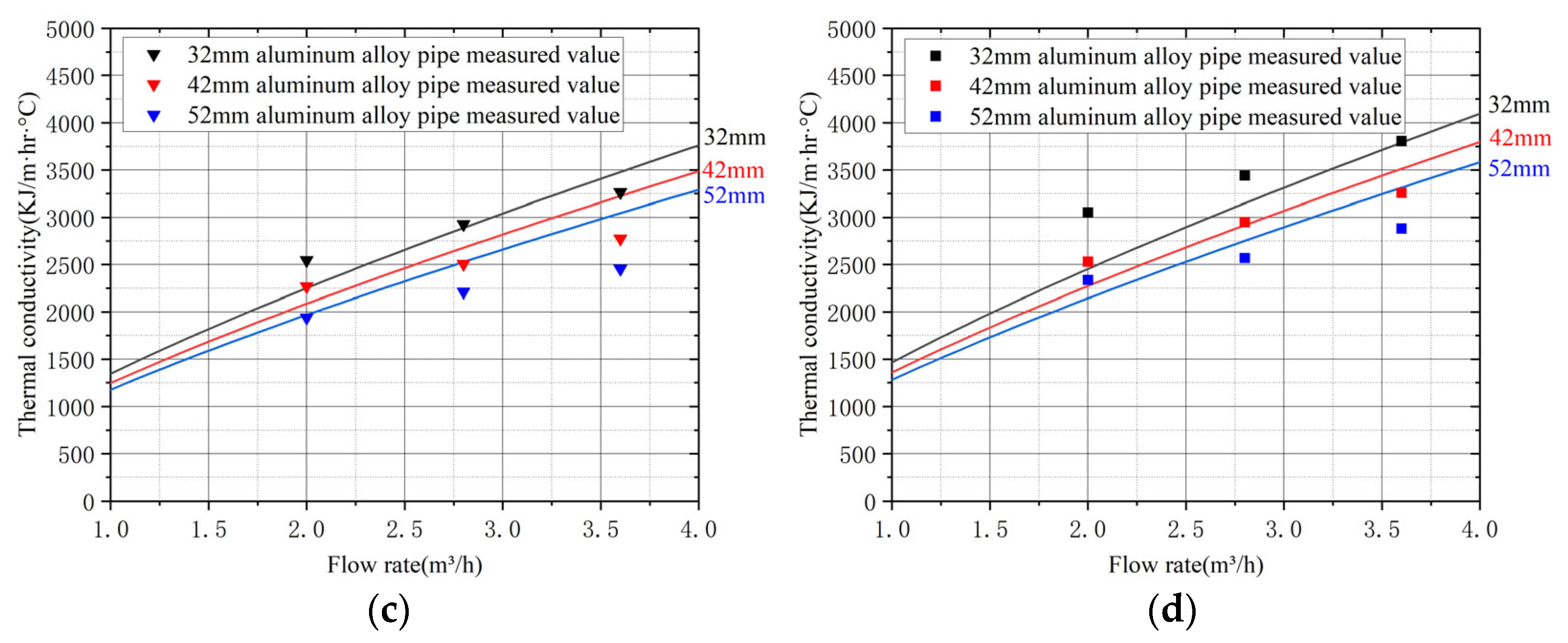
3.3. Effect of the Pipe Diameter on Cooling

The final temperature near the cooling tube decreases more significantly with increasing pipe diameter as shown in Figure 9. At measurement points A3, A5, and A8 (15 cm from the cooling tube), the temperature change with increasing pipe diameter is within 0.3 °C. However, at points closer to the cooling tube, the temperature reduction is more pronounced. When the pipe diameter is increased from 32 mm to 42 mm, the final temperatures at measurement points A2, A4, and A7 (5 cm from the cooling tube) decrease by approximately 1.6 °C, while at points A1 and A6 (attached to the cooling tube wall), the temperatures decrease by 1.8 °C. Further increasing the pipe diameter from 42 mm to 52 mm results in a temperature reduction of approximately 1.3 °C at points A2, A4, and A7, and a similar reduction of 1.4 °C at points A1 and A6.

Increasing the pipe diameter significantly improves cooling efficiency. Such as A1 measuring point, 32 mm diameter cooling from 60 °C to 54.6 °C, for 5.4 °C. When the diameter of the tube is 42 mm, it is cooled from 60 °C to 52.9 °C, which is 7.1 °C. According to the final cooling effect, the cooling effect is increased by 31%. When the pipe diameter is 52 mm, it cools from 60 °C to 51.5 °C, which is 8.5 °C. According to the final cooling effect, the cooling effect is increased by 20%. However, this improvement in cooling efficiency is accompanied by a significant increase in the temperature gradient around the cooling tube, which may increase the risk of thermal cracking.

3.4. Effect of Water Pipe Material on Cooling

As shown in Figure 10, the PVC pipe exhibited the smallest temperature change, with the temperature at point A1 decreasing from 60 °C to 56.55 °C. In contrast, the aluminum alloy pipe showed the largest temperature change, with the temperature at point A1 decreasing from 60 °C to 51.25 °C. The steel pipe’s temperature change was comparable to that of the aluminum alloy pipe, with the temperature at point A1 decreasing from 60 °C to 52.6 °C. The cooling efficiency of the aluminum alloy pipe was 2.5 times that of the PVC pipe, while the steel pipe’s cooling efficiency was 2 times that of the PVC pipe.

The PVC pipe shows good stability during the cooling process, and its cooling rate is relatively low, which can effectively avoid the problem of concrete cracking caused by too fast cooling rate. This kind of pipeline is suitable for construction scenarios with low strength requirements and large concrete volume. For high-strength concrete, since the hydration heat is mainly concentrated in the first two days after pouring, in order to prevent structural damage caused by excessive internal temperature, it is necessary to quickly reduce the maximum temperature inside the concrete. In this case, steel or aluminum alloy tubes are more applicable due to their higher thermal conductivity and cooling efficiency.

The performance of the three types of pipes materials is summarized in

Table 3. The performance of the three pipe materials.

	PVC	Steel	Aluminum Alloy
Cooling Efficiency [Based on PVC]	1	2	2.5
Thermal Conductivity [KJ/m·h °C)]	0.16	54	237
Cracking Risk	Low	Medium	High
Cost (RMB/m)	8	20	40
Recommended Use Case	Crack-sensitive zones	Balanced applications	High-efficiency zones

:

4. Model Validations

The heat transfer between the cooling pipe and the concrete will vary based on factors such as flow rate, the diameter of the pipe, material, arrangement form, and water temperature. It is crucial to take into account the convective heat transfer coefficient under these parameters and establish corresponding calculation models to accurately predict the impact of the cooling tube on the temperature inside mass concrete and control concrete cracking.

The interaction between the water in the tank and the cooling tube in the cooling process is described by the third type of boundary condition, which assumes that the heat transfer between the water in the tank and the cooling tube is directly proportional to the temperature difference.

$$q=\beta (Ta-Tb)$$

(1)

where $Tb$ is the fluid temperature, $q$ is the heat flow, $\beta$ is the convective heat transfer coefficient between the water tank and cooling medium, and $Ta$ is initial temperature.

The initial temperature is 60 °C, the water temperature is 20 °C/30 °C, the cooling tube is a round tube, the radius of the cooling tube is set to $r$, and the unit length of the cooling tube $\mathsf{\Delta }L$ at time $\mathrm{d}t$ in the cooling process is set to remove heat $Q$:

$$dQ=q\cdot \mathrm{d}t\cdot \pi r\cdot \mathsf{\Delta }L$$

(2)

The temperature change T close to the wall of the cooling tube after time t of cooling:

$$T=60-{\displaystyle \frac{{\int }_0^{t}dQ}{c\cdot \rho \cdot \mathsf{\Delta }L\ast \pi r^2}}$$

(3)

where $c$ is the specific heat capacity of the medium outside the tube, $\rho$ is the density of the medium outside the tube.

Equations (1) and (2) are brought into Equation (3) and obtained after collation:

$$\mathrm{Cooling} \mathrm{water} \mathrm{temperature} 20 °\mathrm{C}: T=20+{\displaystyle \frac{40}{1+0.000238\beta t/r}}$$

(4)

$$\mathrm{Cooling} \mathrm{water} \mathrm{temperature} 30 °\mathrm{C}: T=30+{\displaystyle \frac{30}{1+0.000238\beta t/r}}$$

(5)

The convective conductivity coefficients β for the specific conditions of this experiment are presented in

Table 4. Thermal conductivity β table.

Diameter	Material	Temperature	2.0 m3/h	2.8 m3/h	3.6 m3/h
32 mm	Steel	20 °C	2441.25	2776.90	3173.42
		30 °C	2946.23	3312.62	3622.08
	Aluminum	20 °C	2545.80	2927.80	3264.98
		30 °C	3051.2	3440.75	3806.79
42 mm	Steel	20 °C	2120.37	2360.33	2677.48
		30 °C	2444.96	2835.45	3155.77
	Aluminum	20 °C	2269.02	2505.81	2775.76
		30 °C	2531.26	2949.62	3257.57
52 mm	PVC	20 °C	937.99	1045.31	1125.9
		30 °C	950.56	1063.29	1182.42
	Steel	20 °C	1873.65	2149.97	2384.24
		30 °C	2080.89	2400.33	2769.89
	Aluminum	20 °C	1941.35	2213.10	2455.69
		30 °C	2236.64	2569.24	2882.36

as calculated from Equations (4) and (5).

In this study, by designing a water tank arranged with cooling water pipes, the temperature gradient caused by different cooling pipe materials, pipe diameters and cooling water temperatures and flow rates was experimentally investigated to analyze the temperature changes in different cases, and the convection coefficients were obtained from the basic heat transfer equations for each working condition. Since the convection coefficient in actual engineering is affected by many factors, to establish a convection model that considers multiple factors and is more in line with the actual measurements, this paper chooses two models, the parameter identification equation of the Dittus–Boelter equation [12] and the equivalent heat transfer coefficient of Yang Joo-Kyoung [13], and compares the measured experimental results with its results to evaluate the model and the present model. The effect of fitting the model to this experiment, further additions and corrections to the equations, and obtaining the calculation model of heat transfer between concrete and cold pipes using different cases.

4.1. The Dittus–Boelter Equation Parameter Identification Method

The Dittus–Boelter equation is widely utilized in practical engineering to calculate the convection coefficient of cooling water in concrete. This equation takes into account parameters such as the diameter and thermal conductivity of the cooling pipe, flow rate of the cooling water, and temperature. However, it is important to note that these parameters are based on ideal conditions, and the actual thermal field of water pipes in mass concrete can be influenced by numerous unforeseen factors. In a study conducted by Li, an advanced particle swarm optimization technique incorporating particle migration was employed to identify the parameters of the Dittus–Boelter equation within the HFCM using temperature data collected near the Dagangshan Arch Dam. The resulting parameters were then compared with those obtained from experimental results, providing valuable insights for further research in this area.

The Dittus–Boelter equation is widely used to calculate the convective heat transfer coefficient in cooling water pipes, but it is based on several key assumptions. First, the equation assumes fully developed turbulent flow, which is valid for Reynolds numbers (Re) between 10,000 and 200,000 and Prandtl numbers (Pr) between 0.7 and 120. Second, it assumes that the temperature difference between the fluid and the pipe wall is small, which may not hold true in cases where the cooling water temperature is significantly lower than the concrete temperature. Third, the equation does not account for the thermal resistance of the pipe material, which can affect the overall heat transfer efficiency, especially for materials with low thermal conductivity such as PVC. These limitations highlight the need for modifications to the Dittus–Boelter equation when applying it to mass concrete cooling systems, as demonstrated in this study.

4.1.1. The Basic Concept

The Dittus–Boelter equation, originally proposed by Dittus and Boelter [22], is recognized as the predominant equation in engineering for calculating convective heat transfer coefficients in cooling water pipes.

$$N_u=a{R}_e^b{P}_r^c={\displaystyle \frac{\beta d}{{\lambda }_w}}$$

(6)

$$R_e=d{u}_w{\rho }_w/{\mu }_w$$

(7)

$$P_r={\mu }_w{c}_w/{\lambda }_w$$

(8)

The convection coefficient is obtained from the above three equations:

$$\beta =a{R}_e^b{P}_r^c{\lambda }_w/d$$

(9)

where $R_e$ is the Reynolds number, $P_r$ is the Prandtl number, $u_w$ is the cooling water flow rate, $d$ is the tube diameter, ${\mu }_w$ is the cooling water viscosity, $N_u$ is the Nusselt number, ${\rho }_w$ is the cooling water density, $c_w$ is the specific heat of the cooling water, ${\lambda }_w$ is the thermal conductivity of the cooling water, and $a$, $b$, and c are the model coefficients.

The conditions of the Dittus–Boelter equation are as follows: the average temperature of the fluid and the temperature of the concrete are not very different, ${\mathrm{10,000}<R}_e<\mathrm{20,000}$, ${0.7<P}_r<120$, and $L/d\ge 60$; The temperature difference between the concrete and the cooling water typically does not exceed 25 °C., while the standard radius of the water pipe utilized is around 0.02 m; the length of the water pipe is 100~300 m, which can reach $L/d=2380~7142$, $P_r=6.3$, and $R_e=\mathrm{13,427}$; The flow rate of the cooling water meets the requirements of the Dittus–Boelter equation.

This study employs an enhanced particle swarm optimization technique utilizing particle migration to determine the parameters of the Dittus–Boelter equation within the HFCM framework. After inverse calculation, a = 0.026, b = 0.748 and c = 0.361 in Equation (9) are obtained.

The cooling water pipe itself has a certain thermal resistance, and different cooling pipe materials reduce the cooling effect differently, especially the PVC water pipe, so the equivalent heat transfer coefficient ${\beta }_s$ is calculated from the above equation:

$${\beta }_s={\displaystyle \frac{1}{\frac{1}{\beta }+\frac{c_p}{{\lambda }_p}}}$$

(10)

where $c_p$ is the thickness of the water pipe, ${\lambda }_p$ is the thermal conductivity of the water pipe.

4.1.2. Comparison of the Experimental and Calculated Results

The heat transfer coefficient ${\beta }_s$ curves were generated using the parameters from this experiment in Equations (9) and (10), and then compared with the data in Table 4.

Upon comparison with the Dittus–Boelter equation, it is evident from Figure 11 that the measured values for PVC pipes consistently exceed the theoretical values, while the differences between measured and theoretical convection coefficients for PVC pipes are minimal. In contrast, the measured values for steel and aluminum alloy pipes exhibit varying degrees of deviation from their theoretical counterparts.

Based on the empirical data, parameters a, b, and c in Equations (9) and (10) were fine-tuned using the “lsqcurvefit” function in MATLAB R2021b. The optimization process based on MATLAB is described as follows:

(1) The data $R_e$, $P_r$, ${\lambda }_w$, $d$ and $\beta$ are organized as column vectors in MATLAB.

(2) Convert the formula into a functional form.

(3) Using “lsqcurvefit” for least squares fitting.

(4) Calculate predicted values.

The comparison between the optimized curves and the measured values is depicted in Figure 12 The adjusted equations are provided below, and the R² of the fitted Dittus–Boelter equation is 0.899.

For metal pipes, when the water temperature is 20~30 °C, c exhibits a linear difference.

Water temperature is 20 °C: a = 0.625, b = 0.42, c = 0.361

Water temperature is 30 °C: a = 0.625, b = 0.42, c = 0.442

$${\beta }_{m1}={\displaystyle \frac{1}{\frac{1}{a{R}_e^b{P}_r^c{\lambda }_w/d}+\frac{c_p}{{\lambda }_p}}}$$

(11)

For PVC pipes, a, b, and c are the same as for metal pipes:

$${\beta }_{m1}={\displaystyle \frac{1}{\frac{1}{a{R}_e^b{P}_r^c{\lambda }_w/d}+\frac{c_p}{3.926}}}$$

(12)

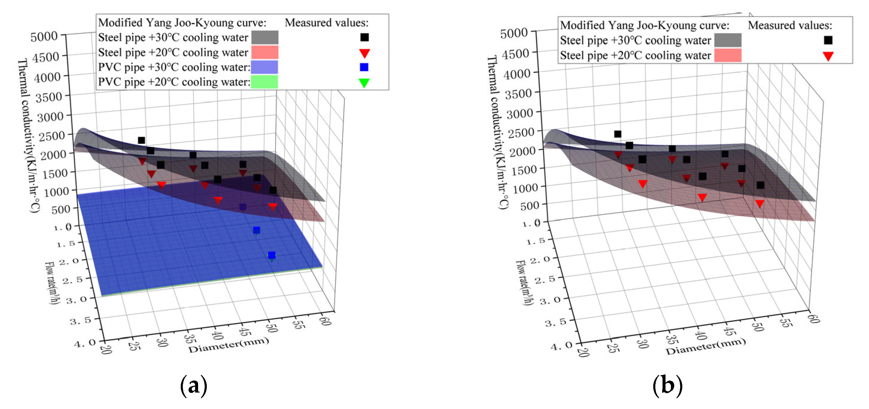
4.2. The Equivalent Heat Transfer Coefficient of Yang Joo-Kyoung

Yang Joo-Kyoung et al. [13] developed a device to measure the heat transfer coefficient based on the concept of internal forced convection. The main factors affecting the heat transfer coefficient in flow convection are the flow velocity, pipe diameter and thickness, and pipe material. A general prediction model for the heat transfer coefficient was proposed by combining the experimental results of the developed device. Yang Joo-Kyoung’s measurement device uses a straight pipe and does not consider the effect of the through-water temperature on heat transfer. The experimental results of this paper are compared and analyzed.

4.2.1. Basic Concept

Based on the concept of internal forced convection, the literature proposes a general prediction model for the heat transfer coefficient based on the main factors affecting the heat transfer coefficient in convection, such as the flow rate, pipe diameter and thickness, and pipe material, and finally obtains the equivalent heat transfer coefficient in Equation (13).

$${\beta }_e={\displaystyle \frac{1}{\frac{r_o\mathrm{l}\mathrm{n}{r}_o/r_i}{k\mathrm{\prime }}+\frac{r_o/r_i}{h_{ideal}}}}$$

(13)

Considering that the equivalent heat transfer coefficient in Equation (13) consists of the cooling water flow rate, the thermal conductivity of the piping material and the piping geometry, such as the outer and inner radii $({\beta }_e=f(r_i,r_o,k_p,u))$, Equation (14) is proposed as a general model for the convective heat transfer coefficient.

$${\beta }_e={\displaystyle \frac{1}{\frac{r_{o}ln{r}_o/r_i}{\alpha k_p}+\frac{r_o/r_i}{1258r_i^{-0.2}{u}^{0.8}}}}$$

(14)

where $k_p$ is the thermal conductivity of the pipe material, $r_i$ is the inner radius of the cooling pipe, $r_o$ is the outer radius of the cooling pipe, and $u$ is the flow rate of the cooling water. $\alpha$ varies with the type of pipe material and the geometry of the pipe and can be used to obtain different values of $\alpha$ according to different cooling pipe materials by using the Equations (15) and (16).

$$\alpha =0.2909{\displaystyle \frac{r_o}{r_i}}-0.2848(\mathrm{for}\mathrm{metal}\mathrm{pipe})$$

(15)

$$\alpha =1.094\hspace{1em}\hspace{1em}(\mathrm{for}\mathrm{PVC}\mathrm{pipe})$$

(16)

4.2.2. Comparison of the Experimental and Calculated Results

The heat transfer coefficient $h_e$ curves for different cooling water pipe parameters are obtained by substituting the parameters used in this experiment into Equation (14) and are compared with the results in Table 4.

Figure 13 depicts a comparison between the Yang Joo-Kyoung equation and the measured values, revealing that the measured values of the PVC pipe consistently surpass the theoretical values. Additionally, there is minimal variation between the measured and theoretical convection coefficient values of the PVC pipe. It should be noted that the Yang Joo-Kyoung equation does not account for through-water temperature effects. Furthermore, when steel pipes are used, measured values generally surpass theoretical values, whereas with aluminum alloy pipes, they tend to fall below theoretical expectations.

From Equations (14)–(16), according to the measured data using the “lsqcurvefit” function in MATLAB to correct $\alpha$, the comparison between the corrected curve and the measured value is illustrated in Figure 14 The corrected equation is as follows, and the R² of the fitted Yang Joo-Kyoung equation is 0.885.

$$\alpha =\left(0.2909{\displaystyle \frac{r_o}{r_i}}-0.2848\right)\times {\displaystyle \frac{\mathrm{10,075.2}}{{\mathsf{\Delta }}_t\times k_p}}(\mathrm{for}\mathrm{metal}\mathrm{pipe})$$

(17)

$$\alpha =5.3252-0.0169\times {\mathsf{\Delta }}_t\hspace{1em}\hspace{1em}(\mathrm{for}\mathrm{PVC}\mathrm{pipe})$$

(18)

where ${\mathsf{\Delta }}_t$ is the disparity between the temperature of the cooling water and the initial temperature.

$${\beta }_{m2}={\displaystyle \frac{1}{\frac{r_{o}ln{r}_o/r_i}{\alpha k_p}+\frac{r_o/r_i}{1258r_i^{-0.2}{u}^{0.8}}}}$$

(19)

4.3. Error Analysis and Limitations

While the experimental setup was designed to minimize errors, several potential sources of error were identified and addressed. First, although insulation material is covered around the water tank, minor heat losses could still occur due to imperfect insulation, which may introduce small errors in the temperature measurements. Since insulation material cannot be installed at the inlet and outlet, a certain amount of temperature loss will also occur. To mitigate this, the insulation was regularly inspected and maintained throughout the experiments. Second, the non-uniform heating of the water tank could lead to temperature variations within the tank, affecting the accuracy of the cooling efficiency measurements. To address this, a high-power water heater with a built-in temperature control system was used to ensure uniform heating. The temperature distribution within the tank was monitored using multiple temperature sensors, and any significant variations were corrected by adjusting the heater settings. Third, external environmental factors, such as ambient temperature fluctuations and air currents, could influence the cooling efficiency and temperature measurements. To minimize these effects, the experiments were conducted in a controlled laboratory environment with stable ambient temperature and humidity.

There are several potential limitations when applying these results to practical engineering. For instance, the thermal properties of concrete, such as thermal conductivity and specific heat, can vary significantly depending on the mix design, aggregate type, and curing conditions. This variability may affect the accuracy of the proposed heat transfer models, particularly in structures with unconventional concrete mixes or additives. Additionally, environmental conditions, such as extreme temperatures, humidity, and wind speed, can influence the cooling efficiency and the risk of thermal cracking. In hot and dry climates, for example, the rapid evaporation of water from the concrete surface may exacerbate temperature gradients and increase the risk of cracking. Conversely, in cold climates, the cooling effect of the pipes may need to be carefully controlled to prevent excessive cooling and potential freezing of the concrete.

5. Application

5.1. General Situation

The heat transfer of two large-volume concrete structures under different working conditions is analyzed and compared with the temperature measured on site to further verify the applicability of the modified formula to the actual heat transfer phenomenon of concrete structures. The measuring points at 1/4 of the structure are arranged as depicted in Figure 15 with positions A1–A3 and B1–B3 (on the same vertical plane as the cooling pipe). The distances from the surface to the upper, middle, and lower measuring points are 0.05 m, 1.5 m, 2.95 m.

The strength grades of the mass concrete structure are C25 (measuring points A1–A3) and C60 (measuring points B1–B3). The cooling pipes are arranged in 42 mm steel tubes with a water flow rate of 3.0 m³/h for 5 days. The pertinent thermodynamic parameters are presented in

Table 5. Thermal properties of the concrete and water.

	C25	C60	Water
Thermal conductivity [KJ/m·h·°C)]	9.927	9.351	2.16
Specific heat [kJ/(kg °C)]	0.896	0.912	4.2
Density [kg/m3]	2430	2480	1000
Coefficient thermal expansion [10−6/°C]	10	10	/
Adiabatic temperature rise [°C)]	35	52.75	/
Poisson’s ratio [−]	0.2	0.2	/

and

Table 6. Mechanical properties of the concrete.

Age	3 d	7 d	14 d	28 d
Compressive strength [MPa]	23.7	26.5	31.9	34.8
Young’s modulus [GPa]	/	/	/	42
Splitting tensile strength [MPa]	2.23	2.51	2.42	3.24

.

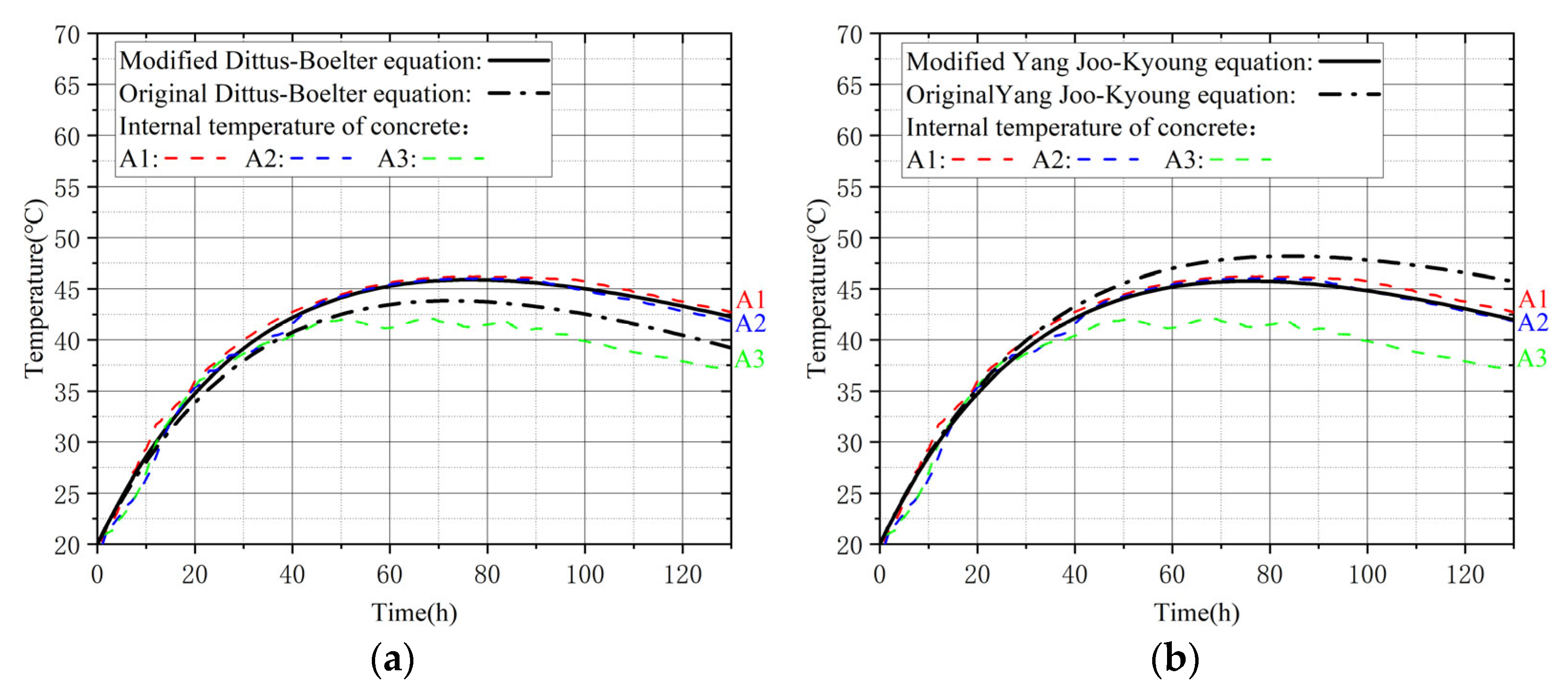
5.2. Comparison Between the Measured Temperature and Modified Formula Temperature

The C25 concrete experiences a temperature rise of 35 °C due to adiabatic conditions, while the molding temperature on the day of casting is 20 °C. Neglecting the cooling effect of internal cooling pipes, the internal temperature of the concrete can be calculated as follows:

$$T=20+35\times (1-e^{-0.027t})$$

(20)

After the embedded cooling tube is used for cooling, the temperature change under the influence of cooling water should be considered. According to the Dittus–Boelter equation modified by Equations (11) and (12), the convection coefficient (${\beta }_{m1}=2496\mathrm{K}\mathrm{J}/\mathrm{m}·\mathrm{h}·°\mathrm{C}$) corresponding to the cooling condition can be obtained.

According to the Yang Joo-Kyoung equation modified by Equations (17)–(19), the convection coefficient (${\beta }_{m2}=2549\mathrm{K}\mathrm{J}/\mathrm{m}·\mathrm{h}·°\mathrm{C}$) corresponding to the cooling condition is obtained.

The convection coefficient is brought into Equations (1) and (2) to obtain the cooling value of the cooling tube. According to Equation (20), the internal temperature change in the concrete under the influence of the cooling tube is finally obtained as follows:

$$T_D=20+35\times (1-e^{-0.027t})-{\displaystyle \frac{{\int }_0^{t}35\beta \pi r(1-e^{-0.027t})dt}{c\cdot \rho \cdot V}}$$

(21)

The calculation process of C60 concrete is the same as above, and the calculation results of Equation (21) are compared with the measured temperature values in the field, as shown in Figure 16 and Figure 17.

Figure 16 shows that measuring points A1–A3 are located within the C25 concrete. A comparison of the calculated results obtained using the modified Dittus–Boelter equation and the modified Yang Joo-Kyoung equation with the measured values at A1 and A2 revealed strong agreement between them. However, it should be noted that the measured values at A3 appear lower than the theoretical values due to influences from external convection effects. Prior to correction, the Dittus–Boelter equation yields excessively large theoretical convection coefficients, resulting in lower calculated temperatures than the actual values, whereas the Yang Jo-Kyoung equation produces overly small coefficients, leading to higher calculated temperatures than the observed temperatures. After being modified, both equations offer enhanced depictions of the internal temperature fluctuations in concrete when cooling pipes are present. It is crucial to consider the impact of external convective heat transfer when approaching the boundaries of concrete structures.

Figure 17 shows that measuring points B1–B3 are located within the C60 concrete. The original Dittus–Boelter equation is smaller than the measured value, and the original Yang Jou-Kyoung equation is larger than the measured value. The calculated results of the modified Dittus–Boelter equation and the modified Yang Jou-Kyoung equation closely align with the measured values. But there is also a certain deviation for the B3 point.

6. Conclusions

In this study, a water tank was designed to study the influence of various factors such as pipe material, pipe diameter, cooling water temperature and flow rate on the cooling of cooling pipes. Then, according to our experimental data, the Dittus–Boelter equation and the Yang Joo-Kyoung equation were modified. Finally, in order to verify the practicability of the modified equation, two concrete blocks were selected for research. The main conclusions are as follows. We can draw the following conclusions:

i.

Among the three types of cooling pipes investigated in this study, aluminum alloy pipes exhibit superior performance, with a cooling efficiency 2.5 times greater than that of PVC pipes. Steel pipes demonstrate a 2 times improvement over PVC pipes, while PVC pipes show relatively slower cooling efficiency.

ii.

Increasing the pipe diameter significantly enhances the overall cooling effect. Specifically, when increasing from 32 mm to 42 mm in diameter, there is a remarkable 31% increase in cooling efficiency; further increasing from 42 mm to 52 mm results in an additional 20% improvement.

iii.

In practical engineering, in order to ensure that the cooling pipe diameter can be fully utilized, it is recommended that the cooling water flow velocity is not less than 0.6 m/s.

iv.

Based on the comparison of the experimental findings with the original Dittus–Boelter equation and the Yang Joo-Kyoung equation, it was observed that the original equation exhibits a relatively large prediction error for PVC pipes, while for steel pipes and aluminum alloy pipes, the error ranges under different conditions. By further refining the modified heat exchange prediction model, estimation of heat transfer coefficients relative to flow and pipeline properties can be achieved.

References

1. Liu, X.; Duan, Y.; Cheng, Y.; Chang, X.; Zhang, C.; Zhou, W. Precise simulation analysis of the thermal field in mass concrete with a pipe water cooling system. Appl. Therm. Eng. 2015, 78, 449–459. [Google Scholar] [CrossRef]
2. Tasri, A.; Susilawati, A. Effect of material of postcooling pipes on temperature and thermal stress in mass concrete. Structures 2019, 20, 204–212. [Google Scholar] [CrossRef]
3. Tasri, A.; Susilawati, A. Effect of cooling water temperature and space between cooling pipes of postcooling system on temperature and thermal stress in mass concrete. J. Build. Eng. 2019, 24, 100731. [Google Scholar] [CrossRef]
4. Pilch, M.; Batog, M.; Klemczak, B.; Żmij, A. Analysis of Cracking Risk in Early Age Mass Concrete with Different Aggregate Types. Procedia Eng. 2017, 193, 234–241. [Google Scholar]
5. Liu, J.; Tian, Q.; Wang, Y.; Li, H.; Xu, W. Evaluation Method and Mitigation Strategies for Shrinkage Cracking of Modern Concrete. Engineering 2021, 7, 348–357. [Google Scholar] [CrossRef]
6. Hu, Y.; Chen, J.; He, M.; Mao, J.; Liu, X.; Zhou, C.; Yuan, Z. A comparative study of temperature of mass concrete placed in August and November based on on-site measurement. Case Stud. Constr. Mater. 2021, 15, e00694. [Google Scholar] [CrossRef]
7. Barnes, L.; Bourchy, A.; Chalencon, F.; Joron, A.; Torrenti, J.M.; Bessette, L. Optimisation of concrete mix design to account for strength and hydration heat in massive concrete structures. Cem. Concr. Compos. 2019, 103, 233–241. [Google Scholar]
8. Zhu, B. Pipe cooling of concrete dam from earlier age with smallertemperature difference and longer time. Water Resour. Hydropower Eng. 2009, 1, 44–50. (In Chinese) [Google Scholar]
9. Myers, G.T.; Fowkes, D.N.; Ballim, Y. Modelling the Cooling of Concrete by Piped Water. J. Eng. Mech. 2009, 135, 1375–1383. [Google Scholar] [CrossRef]
10. Yang, J.; Hu, Y.; Zuo, Z.; Jin, F.; Li, Q. Thermal analysis of mass concrete embedded with double-layer staggered heterogeneous cooling water pipes. Appl. Therm. Eng. 2012, 35, 145–156. [Google Scholar] [CrossRef]
11. Singh, R.P.; Rai, C.D. Effect of Piped Water Cooling on Thermal Stress in Mass Concrete at Early Ages. J. Eng. Mech. 2017, 144, 04017183. [Google Scholar] [CrossRef]
12. Liu, X.; Duan, Y.; Zhou, W.; Chang, X. Modelling the Piped Water Cooling of a Concrete Dam Using the Heat-Fluid Coupling Method. J. Eng. Mech. 2013, 139, 1278–1289. [Google Scholar] [CrossRef]
13. Yang, J.; Lee, Y.; Kim, J. Heat Transfer Coefficient in Flow Convection of Pipe-Cooling System in Massive Concrete. J. Adv. Concr. Technol. 2011, 9, 103–114. [Google Scholar] [CrossRef]
14. Yu, P.; Li, R.; Bie, D.; Liu, X.; Yao, X.; Duan, Y. Precise Simulation of Heat-Flow Coupling of Pipe Cooling in Mass Concrete. Materials 2021, 14, 5142. [Google Scholar] [CrossRef]
15. Chen, S.; Su, P.; Shahrour, I. Composite element algorithm for the thermal analysis of mass concrete Simulation of cooling pipes. Int. J. Numer. Methods Heat Fluid Flow 2011, 21, 434–447. [Google Scholar] [CrossRef]
16. Ding, J.; Chen, S. Simulation and feedback analysis of the temperature field in massive concrete structures containing cooling pipes. Appl. Therm. Eng. 2013, 61, 554–562. [Google Scholar] [CrossRef]
17. Zuo, Z.; Hu, Y.; Li, Q.; Liu, G. An extended finite element method for pipe-embedded plane thermal analysis. Finite Elem. Anal. Des. 2015, 102–103, 52–64. [Google Scholar] [CrossRef]
18. Yudong, X.; Chunxiang, Q. A novel numerical method for predicting the hydration heat of concrete based on thermodynamic model and finite element analysis. Mater. Des. 2023, 226, 111675. [Google Scholar]
19. Nguyen, T.C.; Bui, A.K. The temperature nomogram to predict the maximum temperature in mass concrete. Mag. Civ. Eng. 2024, 17, 12605. [Google Scholar]
20. Seyednavid, M.; Liang, H.C. Prediction of the early age thermal behavior of mass concrete containing SCMs using ANSYS. J. Therm. Anal. Calorim. 2023, 148, 7899–7917. [Google Scholar]
21. Mansour, M.D.; Ebid, M.A. Predicting thermal behavior of mass concrete elements using 3D finite difference model. Asian J. Civ. Eng. 2024, 25, 1601–1611. [Google Scholar] [CrossRef]
22. Dittus, F.W.; Boelter, L.M.K. Heat transfer in automobile radiators of the tubular type. Univ. Calif. Publ. Eng. 1930, 2, 443–461. [Google Scholar] [CrossRef]
Figure 1. Experimental device. (a) Water tank arrangement; (b) TCP-32XL temperature inspector.
Buildings 15 02014 g001
Figure 2. Plumbing diagram.
Buildings 15 02014 g002
Figure 3. Water tank measuring point (mm).
Buildings 15 02014 g003
Figure 4. Cooling tube measuring point (mm).
Buildings 15 02014 g004
Figure 5. The 42 mm aluminum alloy pipe under different cooling water temperatures (20 °C and 30 °C) with a flow rate of 2.8 m3/h. (a) A1, A2, and A3; (b) A4 and A5; (c) A6, A7, and A8.
Buildings 15 02014 g005
Figure 6. The 42 mm aluminum alloy pipe under different cooling water flow rates (2.0 m3/h, 2.8 m3/h, and 3.6 m3/h) with a water temperature of 20 °C. (a) A1, A2, and A3; (b) A4 and A5; (c) A6, A7, and A8.
Buildings 15 02014 g006
Figure 7. The 32 mm aluminum alloy pipe under different cooling water flow rates (2.0 m3/h, 2.8 m3/h, and 3.6 m3/h) with a water temperature of 20 °C. (a) A1, A2, and A3; (b) A4 and A5; (c) A6, A7, and A8.
Buildings 15 02014 g007
Figure 8. The 52 mm aluminum alloy pipe under different cooling water flow rates (2.0 m3/h, 2.8 m3/h, and 3.6 m3/h) with a water temperature of 20 °C. (a) A1, A2, and A3; (b) A4 and A5; (c) A6, A7, and A8.
Buildings 15 02014 g008
Figure 9. Aluminum alloy pipes with different diameters (32 mm, 42 mm, and 52 mm) under a cooling water temperature of 20 °C and a flow rate of 2.8 m3/h. (a) A1, A2, and A3; (b) A4 and A5; (c) A6, A7, and A8.
Buildings 15 02014 g009
Figure 10. Different cooling pipe materials (aluminum alloy, steel, and PVC) with a pipe diameter of 52 mm, a cooling water temperature of 20 °C, and a flow rate of 2.8 m3/h. (a) A1, A2, and A3; (b) A4 and A5; (c) A6, A7, and A8.
Buildings 15 02014 g010
Figure 11. Comparison of the Dittus–Boelter equation with measured values (the solid line is the equation value and the point is the measured value): (a) in 20 °C cooling water for steel and PVC pipes; (b) in 30 °C cooling water for steel and PVC pipes; (c) in 20 °C cooling water for aluminum alloy pipes; (d) in 30 °C cooling water for aluminum alloy pipes.
Buildings 15 02014 g011aBuildings 15 02014 g011b
Figure 12. Comparison between the modified Dittus–Boelter equation and the measured values (the surface is the corrected equation value, and the point is the measured value). (a) Steel and PVC pipes; (b) aluminum alloy tube.
Buildings 15 02014 g012
Figure 13. Comparison of the Yang Joo-Kyoung equation with measured values (the solid line is the equation value and the point is the measured value). (a) Steel and PVC pipes; (b) aluminum alloy tube.
Buildings 15 02014 g013
Figure 14. Comparison between the modified Yang Joo-Kyoung equation and the measured values (the surface is the corrected equation value, and the point is the measured value). (a) Steel and PVC pipes; (b) aluminum alloy tube.
Buildings 15 02014 g014
Figure 15. Concrete structure. (The arrow points to zoom in on the details) (a) Concrete A (C25); (b) Concrete B (C60).
Buildings 15 02014 g015
Figure 16. Comparison of the modified equation and measured values for Concrete A. (a) The Dittus–Boelter equation; (b) the Yang Joo-Kyoung equation.
Buildings 15 02014 g016
Figure 17. Comparison of the modified equation and measured values for Concrete B. (a) The Dittus–Boelter equation; (b) the Yang Joo-Kyoung equation.
Buildings 15 02014 g017