Asphalt and Aggregate Fluorescence Tracing Based on Sensors and Ambient Parameter Optimization

Abstract

Fluorescence tracing effectively identifies asphalt stripping on aggregate surfaces, showing promise for characterizing asphalt–aggregate adhesion in pavement performance detection. However, this method’s effectiveness depends on sensor parameters and ambient conditions. This study developed a fluorescence tracing image acquisition system and employed a five-factor, six-level orthogonal experiment to optimize sensor parameters. We compared multilayer perceptron (MLP) regression, Kolmogorov–Arnold networks regression, and Laplacian sharpening for image quality assessment, with MLP proving superior. The results indicate that (1) image quality is primarily influenced by camera aperture, followed by focal length, exposure time, UV light–camera distance, and object–camera distance; (2) the optimal parameters were 100,000 ms exposure time, 8 mm focal length, 44 cm object–camera distance, aperture of 6, and 30 cm UV light–camera distance; (3) a green background with combined UV and daylight illumination in a glass box yielded the highest image quality score (0.7084); and (4) images acquired under these optimized conditions displayed fluorescence tracing and asphalt regions with superior clarity. This study optimizes the fluorescence tracing method for quantifying the adhesion between asphalt and aggregate and promotes an intellectual approach to material performance detection in pavement engineering.

1. Introduction

The adhesion between asphalt and aggregates is one of the key factors affecting the durability and lifespan of roads [1]. When the adhesion of an asphalt binder decreases, it causes the aggregates to separate from the surface, leading to crack propagation, pothole formation, and a decline in the overall performance of the road structure [2,3]. Therefore, developing reliable methods to assess the adhesion between asphalt and aggregates is crucial for improving the durability of pavement engineering [4].

Various methods have been employed in the engineering field to evaluate the adhesion performance between asphalt and aggregates. (1) The Mechanical Tensile Test System evaluates the adhesion strength between asphalt and aggregates indirectly using tensile (shear) tests, such as pull-off tests, shear adhesion tests, and mechanical tensile peeling tests [5,6,7,8,9,10]. (2) The Surface Energy Evaluation System assesses adhesion by measuring the surface free energy of both asphalt and aggregates. Common methods include contact angle, pendant drop, and Wilhelmy plate methods [11,12,13,14,15,16]. Recently, the application of Atomic Force Microscopy (AFM) has enhanced the precision and reliability of nanoscale analysis [17,18]. (3) The Bonding Area Evaluation System suggests that adhesion occurs not only between asphalt and aggregates but also between asphalt mastic and aggregates. It evaluates adhesion based on interaction indices [4]. (4) The Asphalt Stripping Evaluation System evaluates the exposure level of aggregates after asphalt detachment by applying load or moisture to strip asphalt from aggregate surfaces. It includes qualitative analyses (e.g., boiling water test, immersion test) [19] and quantitative analyses (e.g., photometric method, solvent elution method) [20,21]. Among these, the boiling water test (ASTM D3625) serves as a traditional and experience-driven method that has been around for years [22]. That said, its reliance on visual inspection introduces subjectivity and accuracy limitations.

In recent years, the integration of image processing technology with the boiling water test has transformed the evaluation process from subjective measurement to objective quantification, thus improving the accuracy of assessments [23]. Tayebali et al. proposed a method for analyzing the coating quality of asphalt mixtures after the boiling water test using a colorimeter device [24]. Cui P et al. quantified the degree of asphalt coating on basalt and steel slag particle samples by combining digital image analysis and active adhesion assessment techniques [25]. Arbabpour Bidgoli et al. employed a registered image processing method to analyze the detachment of an asphalt coating under the influence of moisture [26]. However, when the color of the aggregates is similar to that of the asphalt, existing image processing methods struggle to precisely delineate the boundary between the asphalt and aggregates. To address this, Y Peng and colleagues proposed a fluorescence tracing-based BAP (bituminous-coated aggregate particle) image processing technique and developed a new fluorescence tracing method to accurately quantify the loss area of the asphalt coating [27].

The fluorescence tracing method offers significant advantages in evaluating the adhesion between asphalt and aggregates, especially when their colors are similar. However, the current research has not fully considered the impact of camera shooting parameters, sensor placement, and ambient factors on image quality, as well as on the asphalt and fluorescence identification from fluorescence tracing images. To address this gap, this study conducts the following specific tasks, as shown in Figure 1:

• Developing an efficient and stable fluorescence tracing image acquisition system.
• Comparing and evaluating different image quality assessment algorithms to identify a suitable one for this experiment.
• Creating MATLAB^® 2022b programs based on the HVS (hue, saturation, and value) principles to accurately calculate asphalt and fluorescence pixels under UV (ultraviolet) light.
• Determining the optimal parameter combination for the imaging system through orthogonal experiments.
• Investigating ambient factors affecting image quality and optimizing imaging conditions.
• Comparing average fluorescence pixels and average asphalt pixels under different imaging conditions with the optimal setup and analyzing the variations.

2. Materials and Methods

2.1. Material Preparation

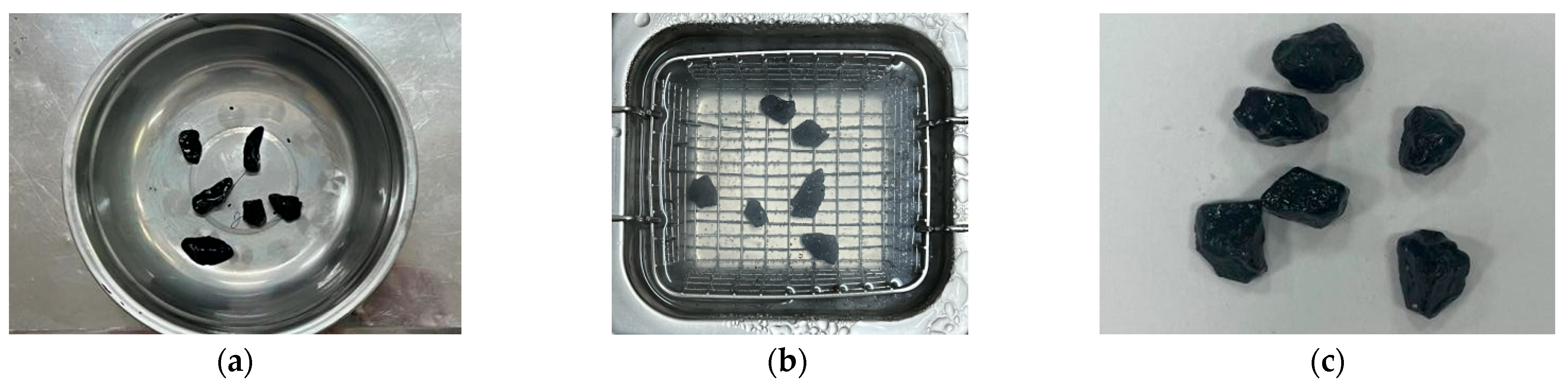
In this study, 70# asphalt was used, and basalt served as the coarse aggregate, with a particle size ranging from 4.75 mm to 9.5 mm. The asphalt stripping tests were conducted following ASTM D3625 and related studies to prepare the BAP (bituminous-coated aggregate particle) samples [22]. The coarse aggregates were dried in a laboratory oven at 105 ± 5 °C for 4–6 h. Meanwhile, the asphalt was heated from 150 °C to 170 °C until it was fully melted. Then, the samples were weighed out to 19.7 g of basalt and blended with asphalt, which accounted for 5.5% ± 0.2% of the aggregate’s total weight. After thorough mixing, the composite was spread evenly onto a tray and cooled to room temperature for later use, as shown in Figure 2a.

Sequentially, the prepared BAP was immersed in a water bath container at 85 ± 5 °C for 30 min. During this process, any asphalt floating on the surface was removed in a timely manner, as shown in Figure 2b. After the test, the specimens were taken out and cooled to room temperature, ensuring that the BAP specimens were in a suitable condition for visual assessment of asphalt stripping. Then, the preparation of the water-damaged specimen was complete, as illustrated in Figure 2c.

2.2. Fluorescence Tracing Method and Imaging Equipment

2.2.1. Fluorescence Tracing of the Asphalt and Aggregate

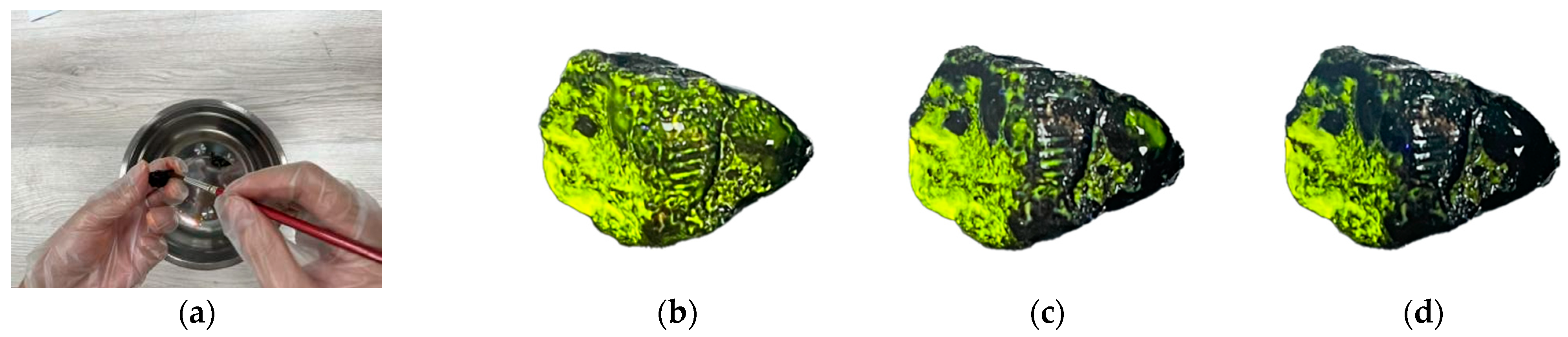
This study was based on related research using fluorescence tracing methods [27]. Fluorescent dye was evenly applied to the surfaces of the BAP samples, with the dye application being moderate, as shown in Figure 3a. Under UV (ultraviolet) light, the surface of the BAP samples exhibits a bright yellow fluorescence effect, as illustrated in Figure 3b. Over time, the fluorescence tracing effect on the asphalt gradually diminishes, while the fluorescence tracing on the aggregate does not significantly weaken, as shown in Figure 3c. After 60 min, the fluorescence effect on the asphalt becomes noticeably weaker, but fluorescence is still observable on the aggregate, as depicted in Figure 3d. Based on this, it is convenient to distinguish between the aggregate and asphalt regions by the distribution of fluorescence, allowing for an accurate assessment of the asphalt stripping rate.

2.2.2. Fluorescence Tracing Image Acquisition System

The fluorescence tracing image acquisition apparatus is shown in Figure 4a and consists primarily of a UV light source, an industrial camera, an aluminum alloy base plate, columns, and a dovetail slide rail platform, among other components. The device allows for precise adjustments of the following parameters: the distance between the camera lens and the sample stage, the horizontal distance between the camera and the UV light source, the angle between the UV light source and the sample stage, and the brightness of the UV light source. These adjustment functions enabled us to independently or collaboratively adjust each parameter to capture the optimal fluorescence images.

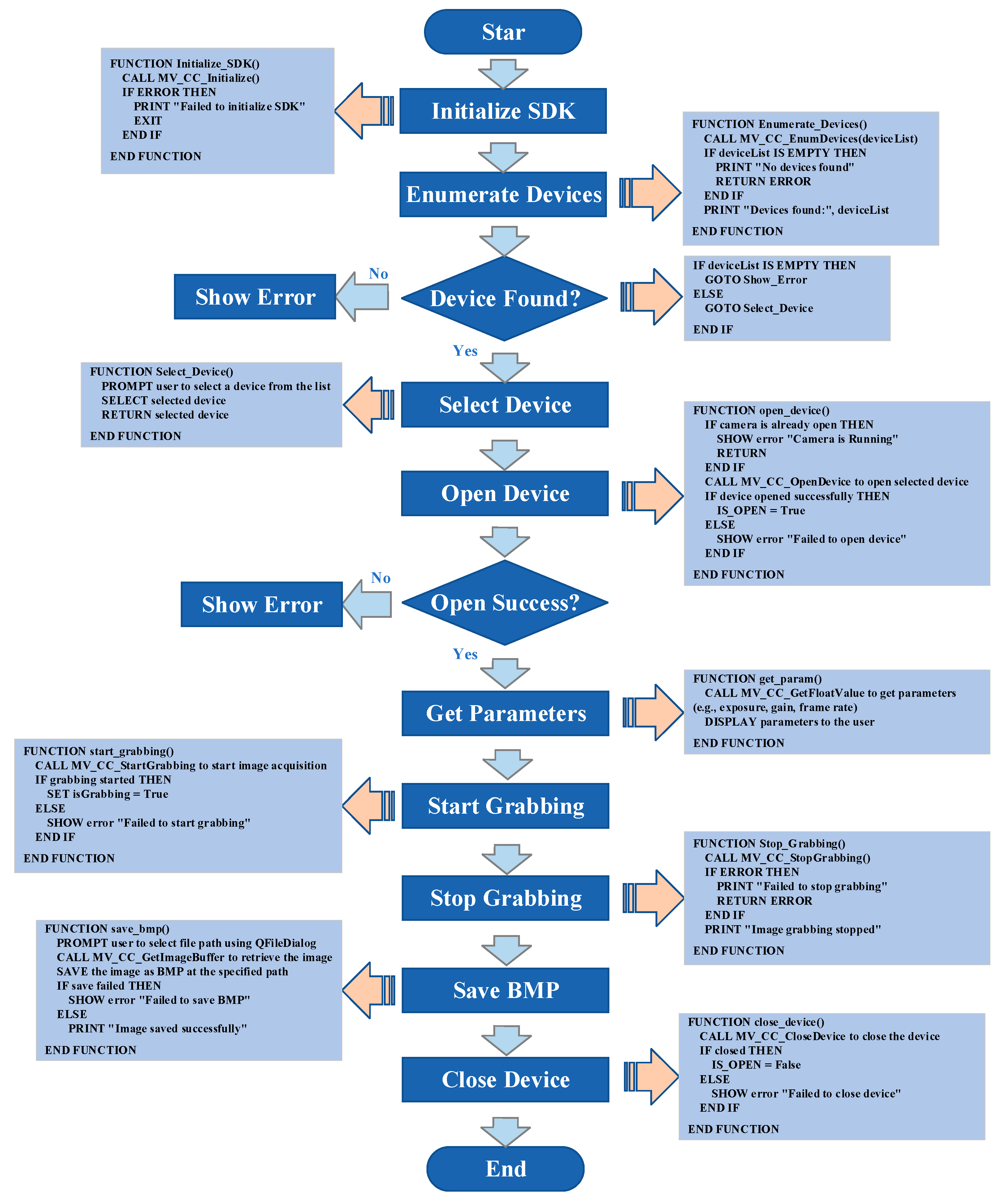
In addition, this research utilized the Haikang Vision SDK 4.1.0 (software development kits), with the programming language Python 3.10 and the GUI (Graphical User Interface) library PyQt5, to develop a set of image acquisition tools. This system provides real-time display and self-defined storage functions for the integrated image management program. The interface is shown in Figure 4b, with the detailed flow of the Haikang^® industrial SDK (manufactured by Haikang Vision, based in Hangzhou, China) for primary data acquisition and corresponding code examples shown in Figure 5.

3. Calibration of a Fluorescence Tracing Imaging System

3.1. Fluorescence Tracing Image Quality Assessment Algorithms

This study obtained fluorescence images by photographing the fluorescence-traced samples under UV light. Researchers [28] recommend assessing image quality with the constraints of lightweight, accurate, and robust no-reference. Thus, the MLP (multilayer perceptron) regression head, the KAN (Kolmogorov–Arnold Network) regression head, and the classical Laplacian sharpness method [29] were adopted to complete this job by means of measuring image sharpness. The MLP and KAN image quality assessment experiments in this study were conducted using the open-source LAR-IQA framework, available on GitHub (https://github.com/nasimjamshidi/LAR-IQA, accessed on 10 March 2025). Specifically, these models were pre-trained and validated in the original LAR-IQA study using multiple public image quality datasets (e.g., KADID-10K, TID2013, KONIQ-10K). In this work, we adopted the released implementations and applied the models directly without retraining. This enabled reliable image quality scoring while leveraging the validated performance of the original framework. The most appropriate image sharpness assessment method was then selected based on a comparative analysis of the effectiveness of all three methods.

(1)

MLP regression.

The MLP regression head uses a traditional multilayer perceptron structure: MLP is one of the traditional neural network architectures. When used for image quality assessment tasks, input image features are processed through a series of fully connected layers and ReLU (Rectified Linear Unit) activation functions, finally generating quality scores [30]. Its image quality evaluation formula is given in Equation (1):

$$\widehat{\mathit{y}}={\mathit{W}}_{\mathbf{2}}\cdot \mathit{R}\mathit{e}\mathit{L}\mathit{U}\left({\mathit{W}}_{\mathbf{1}}\cdot \mathit{x}+{\mathit{b}}_{\mathbf{1}}\right)+{\mathit{b}}_{\mathbf{2}}$$

(1)

where $\widehat{\mathit{y}}$ represents the quality score of the image (namely, the image sharpness), $\mathit{x}$ denotes the image features extracted using MobileNetV3, ${\mathit{W}}_{\mathbf{1}}$ and ${\mathit{W}}_{\mathbf{2}}$ represent the weights of the fully connected layers, ${\mathit{b}}_{\mathbf{1}}$ and ${\mathit{b}}_{\mathbf{2}}$ denote the bias terms, and ReLU refers to the Rectified Linear Unit, which is a nonlinear activation function.

(2)

KAN regression.

The KAN regression head adopts a more complex structure to handle image quality assessment tasks. Unlike the MLP regression head, the KAN regression head utilizes B-spline basis functions and SILU (Sigmoid Linear Unit) activation functions for nonlinear mapping. After the input image features undergo full connection layer processing, they are first compressed to 128 dimensions and then further processed through the nonlinear transformation of KAN, ultimately generating an image quality score [28]. The expression for the image quality assessment of the KAN regression head is presented in Equation (2):

$$\widehat{\mathit{y}}=\sum _{\mathit{i}=\mathbf{1}}^{\mathbf{128}}{\mathit{w}}_{\mathit{i}}\cdot {\mathit{\varphi }}_{\mathit{i}}^{\left(\mathit{l}\right)}\left(\mathit{z}\right)$$

(2)

where $\widehat{\mathit{y}}$ represents the image quality score (namely, the image sharpness), z is an intermediate representation obtained through feature compression, derived from the transformation of input image features after passing through a fully connected layer, and ${\mathit{\varphi }}_{\mathit{i}}^{\left(\mathit{l}\right)}\left(\mathit{z}\right)$ indicates each B-spline basis function applied to the intermediate representation z processed by the SILU activation function and the B-spline basis function. ${\mathit{w}}_{\mathit{i}}$ is the trainable weight for each B-spline basis function, updated during training to adjust the contribution of each basis function to the final image quality score.

(3)

Laplacian operator.

The Laplacian operator method is applied the Laplace transform as a single-index metric for image sharpness assessment. The Laplace transform uses the second derivative of an image to capture its edges and detail information, thereby measuring image sharpness [31]. The Laplacian operator is defined in Equation (3):

$$\mathit{L}\left(\mathit{x},\mathit{y}\right)={\displaystyle \frac{{\mathbf{\partial }}^{\mathbf{2}}\mathit{I}\left(\mathit{x},\mathit{y}\right)}{\mathbf{\partial }{\mathit{x}}^{\mathbf{2}}}}+{\displaystyle \frac{{\mathbf{\partial }}^{\mathbf{2}}\mathit{I}\left(\mathit{x},\mathit{y}\right)}{\mathbf{\partial }{\mathit{y}}^{\mathbf{2}}}}$$

(3)

where $\mathit{I}\left(\mathit{x},\mathit{y}\right)$ represents the grayscale value at pixel point $\left(\mathit{x},\mathit{y}\right)$, and ${\displaystyle \frac{{\mathbf{\partial }}^{\mathbf{2}}}{\partial {\mathit{x}}^{\mathbf{2}}}}$ and ${\displaystyle \frac{{\mathbf{\partial }}^{\mathbf{2}}}{\mathbf{\partial }{\mathit{y}}^{\mathbf{2}}}}$ are the second-order partial derivatives in the horizontal and vertical directions, respectively. In practice, the following 3 × 3 convolution kernel shown in Equation (4) is often used to approximate the Laplacian operator:

$$\mathit{K}=\left[\begin{array}{ccc}0& 1& 0\\ 1& -4& 1\\ 0& 1& 0\end{array}\right]$$

(4)

After obtaining the Laplacian response map $\mathit{L}\left(\mathit{x},\mathit{y}\right)$ through convolution operation, the overall clarity of the image can be quantified by its variance, as defined in Equation (5):

$$Var(L)={\displaystyle \frac{1}{N}}\sum _{x=1}^W\sum _{y=1}^H{\left(L\right(x,y)-{\mu }_L)}^2$$

(5)

where $\mathit{V}\mathit{a}\mathit{r}\left(\mathit{L}\right)$ is the variance (namely, the image sharpness) of the Laplacian response map $\mathit{L}\left(\mathit{x},\mathit{y}\right)$, W and H are the width and height of the image, $\mathit{N}=\mathit{W}\times \mathit{H}$ is the total number of pixels, and ${\mathit{\mu }}_{\mathit{L}}$ is the mean value of the Laplacian response. The larger the variance, the richer the high-frequency details (such as edges and textures) contained in the image. Thus, a higher variance indicates higher image sharpness.

3.2. Fluorescence and Asphalt Region Identification

This section aimed to identify aggregate surface and asphalt areas in fluorescence tracing images and counted the number of pixels in these regions. To achieve this goal, two functions, named the AnalyzeHSV and the CalculatePixels, in MATLAB^® 2022b software were defined to identify the aggregate and asphalt.

Before calling the function, manual background removal was performed on the original image shown in Figure 6a, resulting in the background-free image shown in Figure 6b. Then, the AnalyzeHSV function was used to read the image and convert it into the HSV (hue, saturation, and value) color space [32]. This function calculates the minimum and maximum values of hue (H), saturation (S), and value (V) in the foreground region of the image [33], as shown in Figure 6c. These statistical results reflect the color range of the BAP samples in the image, helping further extract fluorescent regions. The calculated HSV range of the foreground region serves as the basis for subsequent image processing.

In the CalculatePixels function, the HSV range returned by the AnalyzeHSV function is utilized. Based on the set threshold, fluorescent regions were extracted, as shown in Figure 6d. Subsequently, the function employs a dynamic grayscale thresholding method [34], which analyzes the grayscale histogram of the image to automatically calculate a threshold that adapts to the image content. This enables the automatic segmentation of the image regions, thereby extracting the asphalt area. Finally, the function calculates and outputs the pixel counts of the aggregate and asphalt regions.

3.3. Camera and Illumination Parameter Determination Based on Orthogonal Experiment

This section aimed to determine the optimal shooting parameters for the fluorescence tracing system. The orthogonal experiment was designed to select the suitable image quality evaluation methods from the MLP regression head, the KAN regression head, and the Laplacian operator herein. Further, the sensor parameter of the fluorescence tracing system was obtained by a parameter refinement experiment in terms of fine-tuning the experimental factors.

(1)

The orthogonal experiment.

The selected five factors in the orthogonal experiment encompass the exposure time (A) of the camera, the focal length of the camera (B), the height of the camera lens (C), the aperture of the camera (D), and the horizontal distance between the UV light and camera (E).

To effectively investigate the influence of these five experimental factors, each with six levels, we employed the standard orthogonal array L36 (6⁵). This approach significantly reduces the experimental workload compared to a full-factorial design, which would necessitate 7776 experiments, while still maintaining statistical significance. The other orthogonal arrays were not compatible with the factor-level configuration in this study. Consequently, the L36 array provided the optimal balance between comprehensiveness and practicality for our experimental objectives. The image quality assessment method presented in Section 3.1 was employed herein. The experimental factors and their corresponding levels are detailed in

Table 1. Factors and levels of the orthogonal experimental design.

No.	Factor	Level
		1	2	3	4	5	6
(A)	Exposure time (ms)	15,000	30,000	45,000	60,000	75,000	100,000
(B)	Focal length (mm)	0	4	8	12	16	20
(C)	Height of the camera lens (cm)	24	32	40	48	56	64
(D)	Aperture	1	2	3	4	5	6
(E)	The horizontal distance Between the UV light and camera (cm)	10	14	18	22	26	30

Note: Focal length = 0 mm refers to the default minimum setting of the camera without lens extension.

.

The response variable denoted the image quality score. The five factors were assigned different levels. The detailed L36 orthogonal experimental design table is provided in Appendix A.

Range analysis was employed to evaluate the factors of the orthogonal experiment. The range in the analysis was defined as the difference between the extreme values of the data [35]. A larger range indicates a higher sensitivity of the factor to the experimental outcome [36]. The calculation steps for range analysis are given in Equations (6) and (7) [37]:

$${\mathit{k}}_{\mathit{i}\mathit{j}}={\displaystyle \frac{{\mathit{K}}_{\mathit{i}\mathit{j}}}{\mathbf{6}}}$$

(6)

$$\mathit{R}=\mathit{m}\mathit{a}\mathit{x}\left({\mathit{k}}_{\mathit{i}\mathbf{1}},{\mathit{k}}_{\mathit{i}\mathbf{2}},\dots ,{\mathit{k}}_{\mathit{i}\mathbf{6}}\right)-\mathit{m}\mathit{i}\mathit{n}\left({\mathit{k}}_{\mathit{i}\mathbf{1}},{\mathit{k}}_{\mathit{i}\mathbf{2}},\dots ,{\mathit{k}}_{\mathit{i}\mathbf{6}}\right)$$

(7)

where ${\mathit{K}}_{\mathit{i}\mathit{j}}$ and ${\mathit{k}}_{\mathit{i}\mathit{j}}$, respectively, stand for the sum and the average value of the experimental results, which contain the factor $\mathit{i}$ with $\mathit{j}$ level; R represents the range of the factor; $\mathit{m}\mathit{a}\mathit{x}\left({\mathit{k}}_{\mathit{i}1},{\mathit{k}}_{\mathit{i}2},\dots ,{\mathit{k}}_{\mathit{i}\mathit{s}}\right)$ is the highest average value of the factor across all levels; and $\mathit{m}\mathit{i}\mathit{n}\left({\mathit{k}}_{\mathit{i}1},{\mathit{k}}_{\mathit{i}2},\dots ,{\mathit{k}}_{\mathit{i}\mathit{s}}\right)$ is the lowest average value of the factor across all levels.

(2)

Parameter refinement experiment.

Since the preliminary optimal parameters of the fluorescence tracing system and the acceptable fluorescence image quality method were obtained by the above experiment, a follow-up parameter refinement experiment was conducted. The optimal parameters of the fluorescence tracing system were accurately determined by fine-tuning the level of one factor while keeping the other factors unchanged. For example, the levels of factor A were adjusted while the levels of factors B, C, D, and E were kept unchanged. Subsequently, the factors B, C, D, and E were sequentially optimized.

During the fine-tuning process of the parameters, factors A, B, C, D, and E were adjusted up and down with a smaller step size based on the initially determined optimal levels. If the initially optimal levels reached the set maximum or minimum values, corresponding downward or upward adjustments were made.

3.4. Ambient Factor Experimental Design

Previous studies have demonstrated that ambient factors (e.g., illumination conditions) significantly affect image quality [38,39]. Therefore, it is necessary to quantify the influence of ambient factors on the fluorescence tracing image identification.

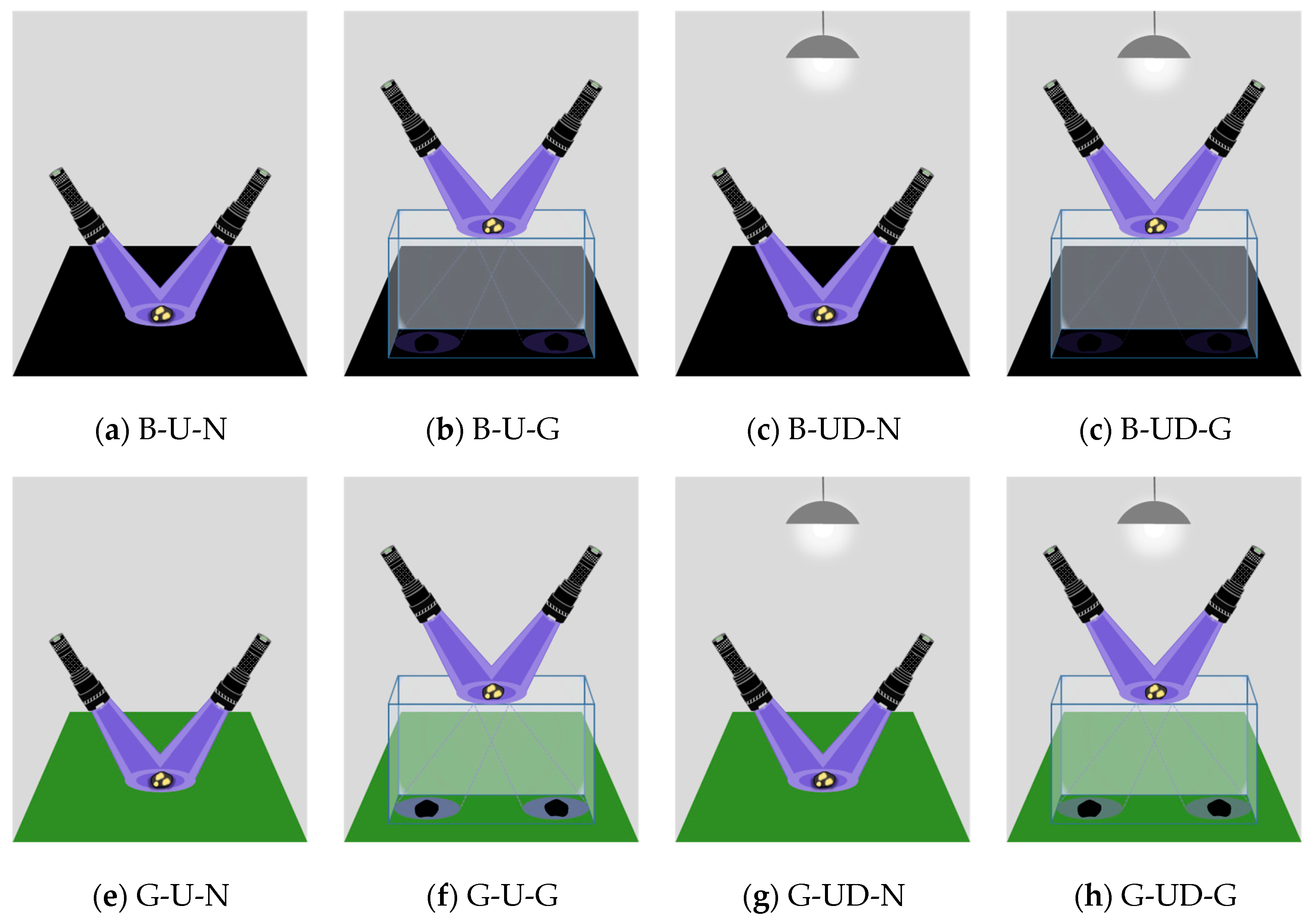
The experiment in this section was based on the optimized fluorescence tracing imaging system and the acceptable image quality evaluation algorithm, both of which were derived from the aforementioned sections. Then, in order to comprehensively evaluate the impact of ambient factors on fluorescence tracing imaging quality, a full factorial experiment was designed concerning the background color (black and green), illumination conditions (UV light and UV light + daylight), and stage transparency (presence or absence of a glass box), as shown in Figure 7. In order to facilitate intuitive visualization of the differences among the three ambient factors (background color, daylight, and glass box) in graphical representations, each factor was uniformly labeled using concise abbreviations. The definitions of the abbreviations are provided in

Table 2. Definitions of abbreviations for ambient conditions.

Abbreviation	Background	Illumination	Stage
B-U-N	Black paper	UV light	None of the Box
B-U-G	Black paper	UV light	Glass Box
B-UD-N	Black paper	UV light + Daylight	None of the Box
B-UD-G	Black paper	UV light + Daylight	Glass Box
G-U-N	Green paper	UV light	None of the Box
G-U-G	Green paper	UV light	Glass Box
G-UD-N	Green paper	UV light + Daylight	None of the Box
G-UD-G	Green paper	UV light + Daylight	Glass Box

.

The ambient factors influencing the image quality were analyzed based on the refined parameters of the fluorescence tracing system and the selected fluorescence image quality assessment method beforehand. This section captured 36 images for each of the 8 ambient conditions, namely, 288 images are prepared in total.

4. Results

4.1. Image Quality Assessment Algorithm Selection

In the determination of the parameters of the image acquisition system, this section employed three distinct algorithms (as shown in Section 3.1 above) to score the 36 sets of photographs captured during the orthogonal experiment. The detailed orthogonal experiment design tables corresponding to each image quality assessment algorithm are presented in Appendix A (

Table A1. Image quality scores using the MLP regression head.

Case	A	B	C	D	E	Image Quality Scores
1	15,000	0	24	1	10	0.3305
2	30,000	20	24	2	18	0.3007
3	45,000	16	24	3	22	0.5805
4	60,000	12	24	4	30	0.6701
5	75,000	8	24	5	10	0.6498
6	100,000	4	24	6	18	0.6555
7	15,000	4	32	2	14	0.3320
8	30,000	0	32	3	22	0.2909
9	45,000	20	32	4	26	0.3791
10	60,000	16	32	5	10	0.6301
11	75,000	12	32	6	14	0.6481
12	100,000	8	32	1	22	0.5954
13	15,000	8	40	3	18	0.6250
14	30,000	4	40	4	26	0.5520
15	45,000	0	40	5	30	0.4786
16	60,000	20	40	6	14	0.5999
17	75,000	16	40	1	18	0.4053
18	100,000	12	40	2	26	0.6008
19	15,000	12	48	4	22	0.2970
20	30,000	8	48	5	30	0.6803
21	45,000	4	48	6	10	0.5914
22	60,000	0	48	1	18	0.3551
23	75,000	20	48	2	22	0.3329
24	100,000	16	48	3	30	0.4781
25	15,000	16	56	5	26	0.3471
26	30,000	12	56	6	10	0.6093
27	45,000	8	56	1	14	0.4479
28	60,000	4	56	2	22	0.5508
29	75,000	0	56	3	26	0.4740
30	100,000	20	56	4	10	0.5273
31	15,000	20	64	6	30	0.4780
32	30,000	16	64	1	14	0.3179
33	45,000	12	64	2	18	0.3717
34	60,000	8	64	3	26	0.6178
35	75,000	4	64	4	30	0.6372
36	100,000	0	64	5	14	0.6037

,

Table A2. Image quality scores using the KAN regression head.

Case	A	B	C	D	E	Image Quality Scores
1	15,000	0	24	1	10	0.6174
2	30,000	20	24	2	18	0.5952
3	45,000	16	24	3	22	0.5833
4	60,000	12	24	4	30	0.5899
5	75,000	8	24	5	10	0.6137
6	100,000	4	24	6	18	0.6119
7	15,000	4	32	2	14	0.6173
8	30,000	0	32	3	22	0.5764
9	45,000	20	32	4	26	0.5737
10	60,000	16	32	5	10	0.5886
11	75,000	12	32	6	14	0.6445
12	100,000	8	32	1	22	0.6044
13	15,000	8	40	3	18	0.6043
14	30,000	4	40	4	26	0.5763
15	45,000	0	40	5	30	0.5549
16	60,000	20	40	6	14	0.5710
17	75,000	16	40	1	18	0.6040
18	100,000	12	40	2	26	0.6019
19	15,000	12	48	4	22	0.5763
20	30,000	8	48	5	30	0.6472
21	45,000	4	48	6	10	0.5779
22	60,000	0	48	1	18	0.5940
23	75,000	20	48	2	22	0.5815
24	100,000	16	48	3	30	0.5890
25	15,000	16	56	5	26	0.5436
26	30,000	12	56	6	10	0.5893
27	45,000	8	56	1	14	0.6168
28	60,000	4	56	2	22	0.6099
29	75,000	0	56	3	26	0.5912
30	100,000	20	56	4	10	0.5655
31	15,000	20	64	6	30	0.5365
32	30,000	16	64	1	14	0.6104
33	45,000	12	64	2	18	0.5935
34	60,000	8	64	3	26	0.6610
35	75,000	4	64	4	30	0.6523
36	100,000	0	64	5	14	0.6221

and

Table A3. Image quality scores based on the Laplacian operator.

Case	A	B	C	D	E	Image Quality Scores
1	15,000	0	24	1	10	0
2	30,000	20	24	2	18	0.0120
3	45,000	16	24	3	22	1.2409
4	60,000	12	24	4	30	6.3075
5	75,000	8	24	5	10	10.5818
6	100,000	4	24	6	18	14.4248
7	15,000	4	32	2	14	0.0007
8	30,000	0	32	3	22	0.0382
9	45,000	20	32	4	26	4.3439
10	60,000	16	32	5	10	9.7514
11	75,000	12	32	6	14	12.2380
12	100,000	8	32	1	22	0.0110
13	15,000	8	40	3	18	0.0095
14	30,000	4	40	4	26	2.1140
15	45,000	0	40	5	30	8.2501
16	60,000	20	40	6	14	11.0371
17	75,000	16	40	1	18	0.0037
18	100,000	12	40	2	26	1.9917
19	15,000	12	48	4	22	0.5980
20	30,000	8	48	5	30	9.1996
21	45,000	4	48	6	10	11.3034
22	60,000	0	48	1	18	0.1898
23	75,000	20	48	2	22	1.6344
24	100,000	16	48	3	30	5.5243
25	15,000	16	56	5	26	3.3744
26	30,000	12	56	6	10	9.2646
27	45,000	8	56	1	14	0.2543
28	60,000	4	56	2	22	1.0252
29	75,000	0	56	3	26	4.6251
30	100,000	20	56	4	10	11.0999
31	15,000	20	64	6	30	10.3437
32	30,000	16	64	1	14	0.0915
33	45,000	12	64	2	18	1.4590
34	60,000	8	64	3	26	4.8969
35	75,000	4	64	4	30	9.6415
36	100,000	0	64	5	14	21.0981

).

Table 3. Results of the range analysis using the MLP regression head.

	A	B	C	D	E
K1	2.4095	2.5328	3.1870	2.4521	3.3384
K2	2.7511	3.3188	2.8756	2.4889	2.9495
K3	2.8492	3.6161	3.2616	3.0662	2.7133
K4	3.4238	3.1970	2.7348	3.0628	2.6474
K5	3.1473	2.7590	2.9564	3.3896	2.9707
K6	3.4607	2.6179	3.0264	3.5821	3.4223
k1	0.4016	0.4221	0.5312	0.4087	0.5564
k2	0.4585	0.5531	0.4793	0.4148	0.4916
k3	0.4749	0.6027	0.5436	0.5110	0.4522
k4	0.5706	0.5328	0.4558	0.5105	0.4412
k5	0.5246	0.4598	0.4927	0.5649	0.4951
k6	0.5768	0.4363	0.5044	0.5970	0.5704
Range R	0.1752	0.1806	0.0878	0.1883	0.1291

Note: The subscripts of K and k represent the level number; the same applies below.

shows that the order of the factors affecting image quality is as follows: aperture (D) > focal length (B) > exposure time (A) > horizontal distance between the UV light and camera (E) > height of the camera lens (C). Based on this order, the initial optimal parameter combination was obtained through extreme difference analysis: A₆B₃C₃D₆E₆. The specific parameters are as follows: exposure time of 100,000 ms, focal length of 8 mm, height of the camera lens of 40 cm, aperture of 6, and horizontal distance between the UV light and camera of 30 cm.

As shown in

Table 4. Results of the range analysis using the KAN regression head.

	A	B	C	D	E
K1	3.4955	3.5559	3.6114	3.6470	3.5526
K2	3.5948	3.6457	3.6049	3.5993	3.6820
K3	3.5000	3.7474	3.5123	3.6051	3.6029
K4	3.6144	3.5954	3.5660	3.5340	3.5318
K5	3.6872	3.5189	3.5163	3.5701	3.5476
K6	3.5948	3.4234	3.6758	3.5311	3.5698
k1	0.5826	0.5927	0.6019	0.6078	0.5921
k2	0.5991	0.6076	0.6008	0.5999	0.6137
k3	0.5833	0.6246	0.5854	0.6009	0.6005
k4	0.6024	0.5992	0.5943	0.5890	0.5886
k5	0.6145	0.5865	0.5860	0.5950	0.5913
k6	0.5991	0.5706	0.6126	0.5885	0.5950
Range R	0.0319	0.0540	0.0272	0.0193	0.0250

, the significance ranking of the various factors affecting image quality is as follows: focal length (B) > exposure time (A) > height of the camera lens (C) > horizontal distance between the UV light and camera (E) > aperture (D). The initial optimal parameter combination is A₅B₃C₆D₁E₂, which corresponds to an exposure time of 75,000 ms, a focal length of 8 mm, a height of the camera lens of 64 cm, an aperture of 1, and a horizontal distance of 14 cm between the UV light and the camera.

As shown in

Table 5. Results of the range analysis using the Laplacian operator.

	A	B	C	D	E
K1	14.3263	34.2014	32.5670	0.5505	52.0010
K2	20.7200	38.5096	26.3833	6.1231	44.7198
K3	26.8517	24.9531	23.4062	16.3349	16.0988
K4	33.2079	31.8588	28.4495	34.1048	4.5478
K5	38.7245	19.9863	29.6435	62.2554	21.3461
K6	54.1499	38.4710	47.5307	68.6116	49.2667
k1	2.3877	5.7002	5.4278	0.0917	8.6668
k2	3.4533	6.4183	4.3972	1.0205	7.4533
k3	4.4753	4.1589	3.9010	2.7225	2.6831
k4	5.5346	5.3098	4.7416	5.6841	0.7580
k5	6.4541	3.3311	4.9406	10.3759	3.5577
k6	9.0250	6.4118	7.9218	11.4353	8.2111
Range R	6.6373	3.0872	4.0208	11.3435	7.9089

, the significance ranking of the various factors affecting image quality is as follows: aperture (D) > horizontal distance between the UV light and camera (E) > exposure time (A) > height of the camera lens (C) > focal length (B). The initial optimal parameter combination is A₆B₂C₆D₆E₁. The specific parameters are as follows: exposure time of 100,000 ms, focal length of 4 mm, height of the camera lens 64 cm, aperture of 6, and the horizontal distance between the UV light and camera of 10 cm.

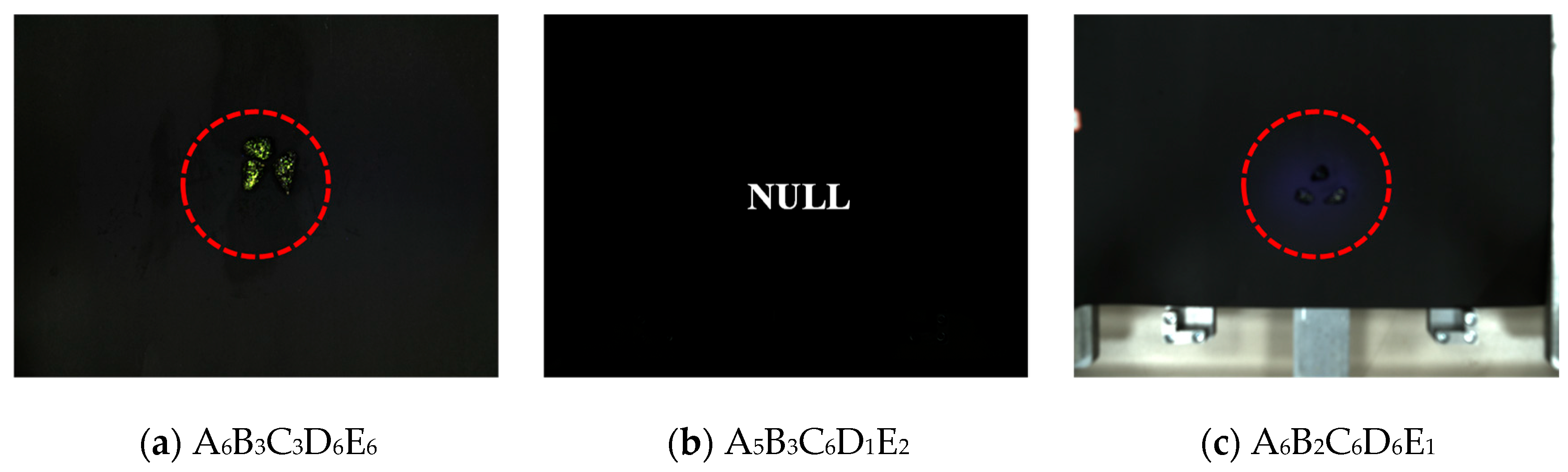
In short, three sets of optimal parameters derived from the orthogonal experiments were employed to capture images, and the comparative results of these images are depicted in Figure 8.

As shown in Figure 8, among the three preliminary optimal parameters obtained from the three image quality assessment algorithms, the images processed with the image quality assessment algorithm utilizing the MLP regression head demonstrated superior sharpness compared to the other two groups. Therefore, for the subsequent parameter refinement experiments, the MLP regression head image quality assessment method was selected.

4.2. Parameter Determination of the Image Acquisition System

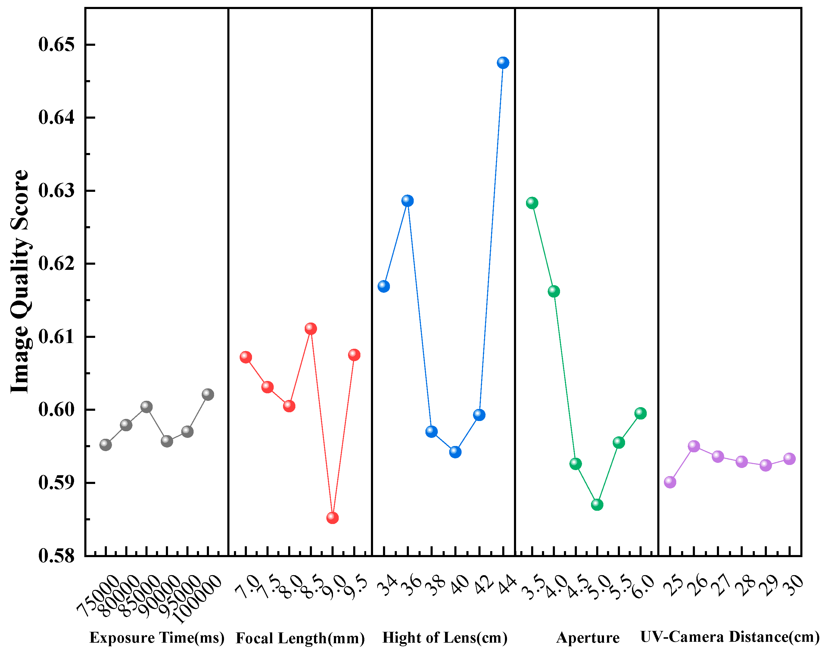
To further improve image quality, a refinement experiment was performed. Other factors were held at their initially optimized levels, while each individual factor was adjusted independently. The resulting image quality score was then calculated as the response variable. The optimization results for each parameter are depicted in Figure 9, illustrating the trend of image quality variation across different parameters, as described below.

The parameter refinement experiments demonstrated that the imaging system achieved the highest image quality score under the parameter combination of exposure time (100,000 ms), focal length (8 mm), height of the camera lens (44 cm), aperture (6), and UV–camera horizontal distance (30 cm), which was superior to the imaging performance obtained with the preliminary optimal parameter set.

4.3. The Impact of Ambient Factors on Image Quality

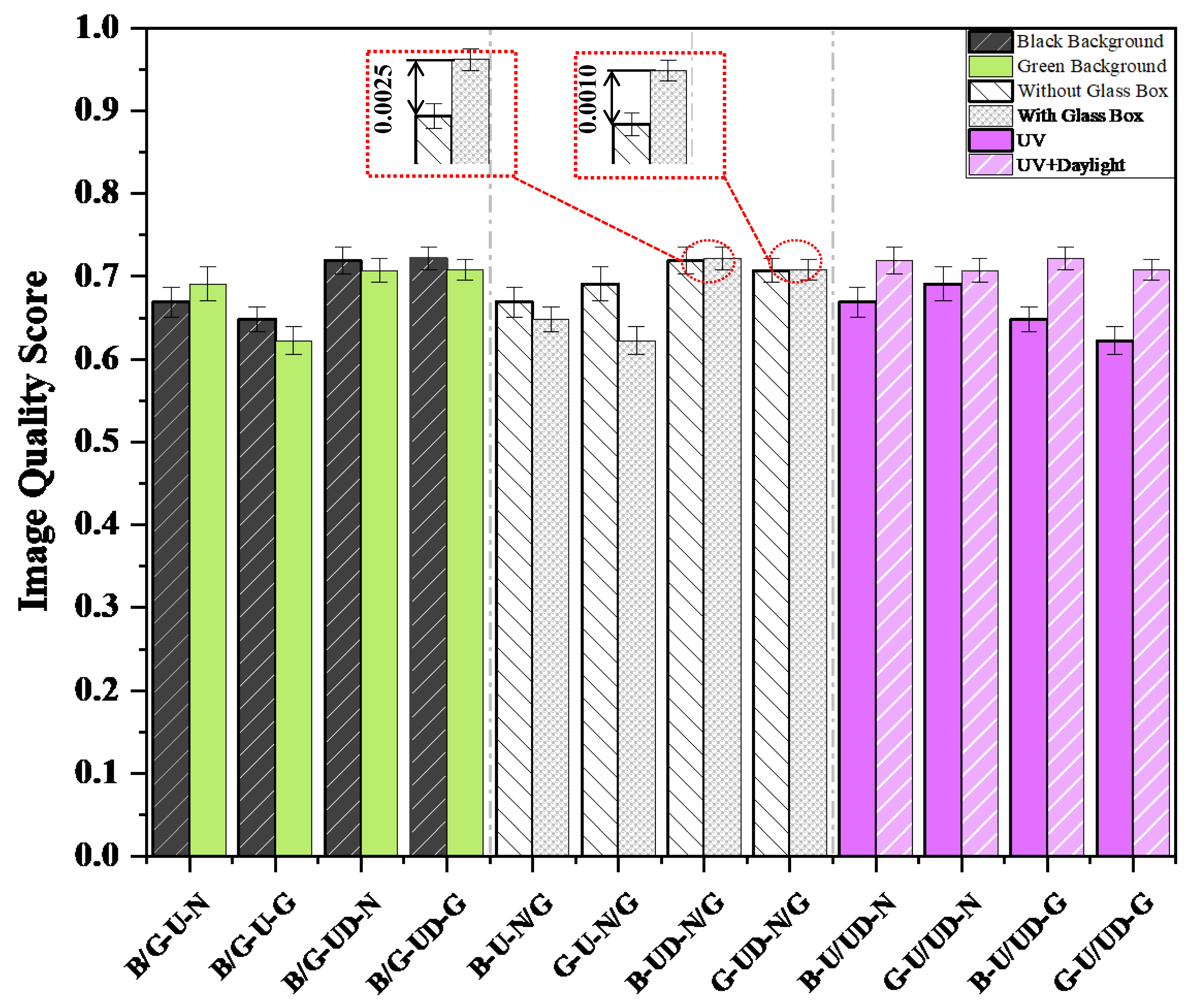
This section examined the changes in image quality when a single environmental variable was altered and explored the regularities underlying these changes. Figure 10 presents the image quality scores under the variation in a single factor.

(1)

Impact of the Background Color.

In the comparative study of background colors, the image quality scores with a black background were generally higher than those with a green background. The highest score for the black background was 0.7217, compared to 0.7084 for the green background, indicating that the black background scores were 1.88% higher than the green background.

(2)

Impact of the Glass Box.

In the absence of daylight (UV light), the environment without a glass box scored an average of 7.13% higher than that with a glass box, indicating that the glass box results in lower image quality in the absence of daylight. With the daylight on (UV light + daylight), the environment with a glass box scored an average of 0.24% higher than that without a glass box, suggesting that the glass box has a minimal impact on image quality when lighting is present.

(3)

Impact of Lighting Conditions.

The introduction of daylight (UV light + daylight) significantly improved image quality, with scores averaging an 8.73% increase compared to the conditions without daylight.

Based on the above analysis, the final configuration adopted was G-UD-G (green background, UV light + daylight, glass box), which not only yielded a higher image quality score (0.7084) but also provided higher chromatic contrast with the green background. Moreover, the glass box effectively eliminated shadows, enhancing the stability of the images. These advantages can significantly reduce the complexity of subsequent image processing, such as segmentation and fluorescence region extraction, thereby providing a more reliable basis for further analysis.

4.4. The Effect of Ambient Factors on the Average Pixels of the BAP Samples

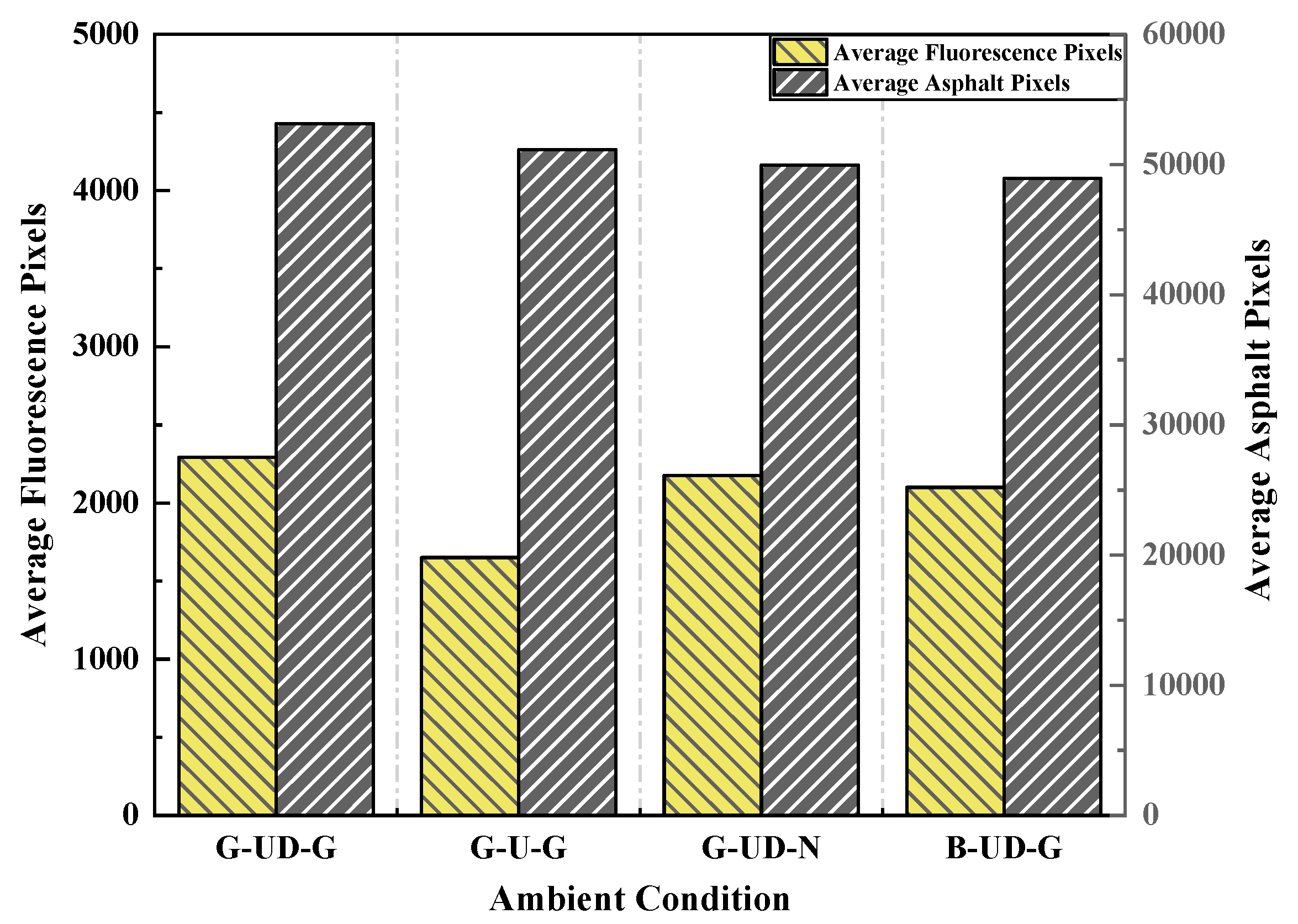
In this section, environmental factors such as lighting, the presence or absence of a glass box, and background color were individually adjusted. Under these varying conditions, images of all six faces of six BAP samples were captured. The average fluorescence and asphalt pixels were then extracted and calculated from the images, with the statistical results presented in Figure 11.

As depicted in Figure 11, the number of fluorescent pixels and asphalt pixels captured by the camera varies significantly under different conditions. For instance, under the background condition G-UD-G, which offers the highest clarity, the average number of fluorescent pixels recorded is 2293. In contrast, the conditions G-U-G, G-UD-N, and B-UD-G exhibit decreases of 643, 118, and 193 pixels, respectively, compared to G-UD-G. Similarly, the average number of asphalt pixels under G-UD-G is 53145, while G-U-G, G-UD-N, and B-UD-G show reductions of 2001, 3198, and 4222 pixels, respectively. These findings indicate that under the optimal background condition, both fluorescent and asphalt features are more distinctly recognizable by the camera.

5. Discussion

While this study primarily focuses on fluorescence tracing for individual bitumen-coated aggregate particles (BAPs), we recognize the importance of extending the method to more complex specimens, such as asphalt mixture samples. Specifically, materials like rutting slabs and Marshall samples, which contain multiple aggregates and varied surface roughness, pose challenges for image processing and accurate adhesion assessment.

The proposed fluorescence imaging system was optimized for individual BAPs under controlled laboratory conditions. However, given its modular setup, the system has the potential to be adapted for assessing adhesion in asphalt mixtures by adjusting key parameters such as exposure time, focal length, ambient lighting, and background conditions. This flexibility makes the system suitable for different types of asphalt mixtures, as long as adjustments to imaging parameters are made to accommodate the increased surface variability and complexity of the specimens.

Despite the promising potential, the challenge remains in the heterogeneity in asphalt mixtures. Unlike single aggregate particles, asphalt mixtures have multiple aggregate types with different shapes, sizes, and surface roughness, which can impact the fluorescence intensity and distribution. Additionally, the non-uniformity of fluorescence signals across different aggregates in a mixture can make it difficult to accurately assess adhesion without further algorithmic development.

Future work will focus on refining the image processing algorithms to handle these complexities effectively. Specifically, the algorithms will need to account for the increased texture variation, surface irregularities, and optical differences between different types of aggregates in the mixture. Validation of the method will also be conducted with larger asphalt mixture samples, including those used in field settings, to ensure the system’s reliability and scalability.

Moreover, further studies will explore the replicability of the proposed method under real-world conditions, such as varying ambient lighting, non-ideal imaging angles, and different asphalt mixture compositions. By refining these aspects, we aim to improve the system’s applicability for practical use in quality assurance/quality control processes at asphalt mixing plants, as well as in forensic analysis of pavement failures.

6. Conclusions

This study developed a comprehensive fluorescence tracing image acquisition system by integrating orthogonal experimental design with image quality assessment algorithms. Through a systematic five-factor, six-level orthogonal experiment, an acceptable image quality assessment algorithm was identified for the specific requirements. Parameter refinement experiments were conducted to enhance image quality. The investigation extended beyond parameter optimization to explore the influence of ambient factors on both image quality and pixel point measurements of the fluorescence-traced asphalt mixture image. The key findings of this research are as follows:

(1)

Among the image quality assessment algorithms, i.e., the MLP regression head, the KAN regression head, and the Laplacian operator sharpness assessment method, the MLP regression head demonstrated the best performance in fluorescence tracing experiments.

(2)

Through the five-factor, six-level orthogonal experiment and range analysis, the significance of each factor on image quality was ranked as follows: aperture (D) > focal length (B) > exposure time (A) > horizontal distance between the UV light and camera (E) > height of the camera lens (C).

(3)

Through orthogonal experimentation, the optimized parameter combination was identified as follows: exposure time of 100,000 ms, focal length of 8 mm, height of the camera lens of 44 cm, aperture of 6, and the horizontal distance between the UV light and the camera of 30 cm.

(4)

Under the G-UD-G condition, which uses a green background, UV light + daylight, and a glass box, ambient factor analysis showed that the image quality score was relatively high (score = 0.7084), ensuring image clarity and stability.

(5)

The optimized background conditions G-UD-G significantly enhance the camera’s ability to capture fluorescent and asphalt pixels, resulting in clearer feature recognition.

This research provides specific guidelines for applying fluorescence tracing methods to quantify asphalt–aggregate adhesion, with particular emphasis on image quality optimization. The findings demonstrate that optimized capture parameters and controlled ambient conditions significantly enhance fluorescence image quality while minimizing external interference. Moreover, these methodological advancements offer broad applications in moisture damage assessment of asphalt and aggregate mixtures, pavement durability evaluation, and practical scenarios, such as quality assurance/quality control procedures in asphalt mixing plants and forensic analysis of pavement failures, as well as other related civil engineering fields.

References

- Guo, F.; Pei, J.; Zhang, J.; Xue, B.; Sun, G.; Li, R. Study on the adhesion property between asphalt binder and aggregate: A state-of-the-art review. Constr. Build. Mater. 2020, 256, 119474. [Google Scholar] [CrossRef]
- Cong, P.; Guo, X.; Ge, W. Effects of moisture on the bonding performance of asphalt-aggregate system. Constr. Build. Mater. 2021, 295, 123667. [Google Scholar] [CrossRef]
- Cui, W.T. Moisture-Induced Failure of Adhesion Performance at the Asphalt-Aggregate Interface. Master’s Thesis, Guangzhou University, Guangzhou, China, 2021. [Google Scholar] [CrossRef]
- Huang, G.; Zhang, J.; Wang, Z.; Guo, F.; Li, Y.; Wang, L.; He, Y.; Xu, Z.; Huang, X. Evaluation of asphalt-aggregate adhesive property and its correlation with the interaction behavior. Constr. Build. Mater. 2023, 374, 130909. [Google Scholar] [CrossRef]
- Alkofahi, N.; Khedaywi, T. Stripping Potential of Asphalt Mixtures: State of the Art. Int. J. Pavement Res. Technol. 2021, 15, 29–43. [Google Scholar] [CrossRef]
- Dong, M.; Sun, B.; Thom, N.; Li, L. Characterisation of temperature and loading rate dependent bond strength on the Bitumen-aggregate interface using direct shear test. Constr. Build. Mater. 2023, 394, 132284. [Google Scholar] [CrossRef]
- Liddell, H.P.H.; Erickson, L.M.; Tagert, J.P.; Arcari, A.; Smith, G.M.; Martin, J. Mode mixity and fracture in pull-off adhesion tests. Eng. Fract. Mech. 2023, 281, 109120. [Google Scholar] [CrossRef]
- Rahim, A.; Thom, N.; Airey, G. Development of compression pull-off test (CPOT) to assess bond strength of bitumen. Constr. Build. Mater. 2019, 207, 412–421. [Google Scholar] [CrossRef]
- Sek Yee, T.; Hamzah, M.O.; Van den Bergh, W. Evaluation of moisture susceptibility of asphalt-aggregate constituents subjected to direct tensile test using imaging technique. Constr. Build. Mater. 2019, 227, 116642. [Google Scholar] [CrossRef]
- Zhou, L.; Huang, W.; Xiao, F.; Lv, Q. Shear adhesion evaluation of various modified asphalt binders by an innovative testing method. Constr. Build. Mater. 2018, 183, 253–263. [Google Scholar] [CrossRef]
- Caputo, P.; Miriello, D.; Bloise, A.; Baldino, N.; Mileti, O.; Ranieri, G.A. A comparison and correlation between bitumen adhesion evaluation test methods, boiling and contact angle tests. Int. J. Adhes. Adhes. 2020, 102, 102680. [Google Scholar] [CrossRef]
- Haghshenas Hamzeh, F.; Rea, R.; Reinke, G.; Yousefi, A.; Haghshenas Davoud, F.; Ayar, P. Effect of Recycling Agents on the Resistance of Asphalt Binders to Cracking and Moisture Damage. J. Mater. Civ. Eng. 2021, 33, 04021292. [Google Scholar] [CrossRef]
- Tu, C.; Luo, R.; Huang, T. Influence of Infiltration Velocity on the Measurement of the Surface Energy Components of Asphalt Binders Using the Wilhelmy Plate Method. J. Mater. Civ. Eng. 2021, 33, 04021243. [Google Scholar] [CrossRef]
- Wang, Y.-Z.; Shi, J.-T.; Wang, X.-D.; Yang, G. Research on Adhesive Properties between Asphalt and Aggregates at High Temperature. J. Highw. Transp. Res. Dev. 2020, 14, 53–62. [Google Scholar] [CrossRef]
- Xu, O.; Xiang, S.; Yang, X.; Liu, Y. Estimation of the surface free energy and moisture susceptibility of asphalt mastic and aggregate system containing salt storage additive. Constr. Build. Mater. 2022, 318, 125814. [Google Scholar] [CrossRef]
- Zhu, S.; Kong, L.; Peng, Y.; Chen, Y.; Zhao, T.; Jian, O.; Zhao, P.; Sheng, X.; Li, Z. Mechanisms of interface electrostatic potential induced asphalt-aggregate adhesion. Constr. Build. Mater. 2024, 438, 137255. [Google Scholar] [CrossRef]
- Ji, X.; Hou, Y.; Zou, H.; Chen, B.; Jiang, Y. Study of surface microscopic properties of asphalt based on atomic force microscopy. Constr. Build. Mater. 2020, 242, 118025. [Google Scholar] [CrossRef]
- Sun, E.; Zhao, Y.; Cai, R. Characterization of microstructural evolution of asphalt due to water damage using atomic force microscopy. Constr. Build. Mater. 2024, 438, 137175. [Google Scholar] [CrossRef]
- Liu, X.; Chen, S.; Ma, T.; Wu, X.; Yang, J. Investigation of Adhesion Property between Asphalt Binder and Aggregate Using Modified Boiling Methods for Hot and Wet Area. J. Mater. Civ. Eng. 2023, 35, 04022467. [Google Scholar] [CrossRef]
- Geng, J.; Sun, X.; Chen, M.; Lan, Q.; Wang, W.; Kuang, D. Relationship of Adhesion Performance between Asphalt Binder Using Solvent Elution Method and Crushed Pebbles Asphalt Mixture. J. Mater. Civ. Eng. 2022, 34, 04022162. [Google Scholar] [CrossRef]
- Wang, H.; Chen, G.; Kang, H.; Zhang, J.; Rui, L.; Lyu, L.; Pei, J. Asphalt-aggregates interface interaction: Correlating oxide composition and morphology with adhesion. Constr. Build. Mater. 2024, 457, 139317. [Google Scholar] [CrossRef]
- Xiao, R.; Polaczyk, P.; Wang, Y.; Ma, Y.; Lu, H.; Huang, B. Measuring moisture damage of hot-mix asphalt (HMA) by digital imaging-assisted modified boiling test (ASTM D3625): Recent advancements and further investigation. Constr. Build. Mater. 2022, 350, 128855. [Google Scholar] [CrossRef]
- Esmaeili, R.; Javadi, S.; Jamshidi, H.; Esmaeili Taheri, M.; Khani Sanij, H. Stripping propensity detection of HMA Mixes: With focus on image processing method. Constr. Build. Mater. 2022, 352, 129022. [Google Scholar] [CrossRef]
- Tayebali, A.A.; Kusam, A.; Bacchi, C. An Innovative Method for Interpretation of Asphalt Boil Test. J. Test. Eval. 2018, 46, 1622–1635. [Google Scholar] [CrossRef]
- Cui, P.; Wu, S.; Xiao, Y.; Wang, F.; Wang, F. Quantitative evaluation of active based adhesion in Aggregate-Asphalt by digital image analysis. J. Adhes. Sci. Technol. 2019, 33, 1544–1557. [Google Scholar] [CrossRef]
- Arbabpour Bidgoli, M.; Hajikarimi, P.; Pourebrahimi Mohammad, R.; Naderi, K.; Golroo, A.; Moghadas Nejad, F. Introducing Adhesion–Cohesion Index to Evaluate Moisture Susceptibility of Asphalt Mixtures Using a Registration Image-Processing Method. J. Mater. Civ. Eng. 2020, 32, 04020376. [Google Scholar] [CrossRef]
- Peng, Y.; Zhao, T.; Zeng, Q.; Deng, L.; Kong, L.; Ma, T.; Zhao, Y. Interpretation of stripping at the bitumen–aggregate interface based on fluorescence tracing method. J. Mater. Res. Technol. 2023, 25, 5767–5780. [Google Scholar] [CrossRef]
- Jamshidi Avanaki, N.; Ghildyal, A.; Barman, N.; Zadtootaghaj, S.J.a.e.-p. LAR-IQA: A Lightweight, Accurate, and Robust No-Reference Image Quality Assessment Model. arXiv 2024, arXiv:2408.17057. [Google Scholar] [CrossRef]
- Fuentes-Carbajal, J.A.; Carrasco-Ochoa, J.A.; Martínez-Trinidad, J.F.; Flores-López, J.A. Machine Learning and Image-Processing-Based Method for the Detection of Archaeological Structures in Areas with Large Amounts of Vegetation Using Satellite Images. Appl. Sci. 2023, 13, 6663. [Google Scholar] [CrossRef]
- Sendjasni, A.; Larabi, M.-C. PW-360IQA: Perceptually-Weighted Multichannel CNN for Blind 360-Degree Image Quality Assessment. Sensors 2023, 23, 4242. [Google Scholar] [CrossRef]
- Zhu, M.; Yu, L.; Wang, Z.; Ke, Z.; Zhi, C. Review: A Survey on Objective Evaluation of Image Sharpness. Appl. Sci. 2023, 13, 2652. [Google Scholar] [CrossRef]
- Lv, C.; Li, J.; Kou, Q.; Zhuang, H.; Tang, S. Stereo Matching Algorithm Based on HSV Color Space and Improved Census Transform. Math. Probl. Eng. 2021, 2021, 1857327. [Google Scholar] [CrossRef]
- Waldamichael, F.G.; Debelee, T.G.; Ayano, Y.M. Coffee disease detection using a robust HSV color-based segmentation and transfer learning for use on smartphones. Int. J. Intell. Syst. 2022, 37, 4967–4993. [Google Scholar] [CrossRef]
- Li, J.; Gui, X. Fully Automatic Grayscale Image Segmentation: Dynamic Thresholding for Background Adaptation, Improved Image Center Point Selection, and Noise-Resilient Start/End Point Determination. Appl. Sci. 2024, 14, 9303. [Google Scholar] [CrossRef]
- Xie, N.; Wei, W.; Ba, J.; Yang, T. Operation parameters study on the performance of PEMFC based orthogonal test method. Case Stud. Therm. Eng. 2024, 61, 105035. [Google Scholar] [CrossRef]
- Gao, X.; Zhang, Y.; Zhang, H.; Wu, Q. Effects of Machine Tool Configuration on Its Dynamics Based on Orthogonal Experiment Method. Chin. J. Aeronaut. 2012, 25, 285–291. [Google Scholar] [CrossRef]
- Zou, G.; Xu, J.; Wu, C. Evaluation of factors that affect rutting resistance of asphalt mixes by orthogonal experiment design. Int. J. Pavement Res. Technol. 2017, 10, 282–288. [Google Scholar] [CrossRef]
- Arad, B.; Kurtser, P.; Barnea, E.; Harel, B.; Edan, Y.; Ben-Shahar, O. Controlled Lighting and Illumination-Independent Target Detection for Real-Time Cost-Efficient Applications. The Case Study of Sweet Pepper Robotic Harvesting. Sensors 2019, 19, 1390. [Google Scholar] [CrossRef]
- Feng, X.; Li, J.; Hua, Z.; Zhang, F. Low-light image enhancement based on multi-illumination estimation. Appl. Intell. 2021, 51, 5111–5131. [Google Scholar] [CrossRef]