Study on Semi-Rigid Joint Performance and Stability Bearing Capacity of Disc-Type Steel Pipe Support

Abstract

The current lack of standardized calculation methods for disc-buckle-type steel pipe supports, coupled with unsafe calculation length coefficients, has resulted in frequent safety incidents leading to severe casualties and economic losses. In this paper, the semi-rigidity characteristics of joints were investigated through the field bending test of disc-buckle steel pipe supports. Through analysis of the bending moment–rotation curves obtained from these tests, accurate initial bending stiffness values and a calculation model for semi-rigid joints were established. Numerical simulation and analytical correction method were employed to determine the effective length correction coefficient ${\mathsf{\mu }}_0$ under various erection parameters while accounting for joint semi-rigidity. The findings indicate that the slenderness ratio derived by the revised effective length coefficient is 8.13% greater than the standard value, primarily because current standards fail to adequately consider the constraint effect of the crossbar. The correction coefficient proposed in this paper provides a theoretical foundation for the safe construction of disc-type steel pipe supports, and holds significant value for engineering applications.

1. Introduction

Disc-buckle-type steel pipe supports have been extensively adopted in contemporary construction engineering due to their advantages of expeditious installation, substantial load-bearing capacity, and superior self-locking performance [1,2]. Nevertheless, collapse incidents involving steel pipe supports are frequently reported during both construction and operational phases [3]. This can be primarily attributed to insufficient research regarding the joint stiffness values within the disc-type steel pipe support system, which has consequently led to inadequate understanding of the overall stability characteristics of these supports [4,5]. According to statistical data from AISC 360-22, approximately 30% of scaffold collapse incidents are attributed to inaccurate estimation of joint connection stiffness. This indicates a significant discrepancy between the stiffness assumptions specified in current codes and the actual mechanical behavior of rosette-type steel tube scaffold joints in engineering practice [6]. Therefore, investigating the semi-rigid properties of bolted joints and their influence on support stability is of considerable theoretical and practical significance, as it provides crucial safety assurances for implementation in actual construction projects.

The effective length coefficient in the Euler formula is determined according to the boundary constraints of the structural member. However, compression members with true pinned connections at both ends are rarely encountered in practice, and the analysis must account for the constraints imposed by interconnected members [7]. The calculation length coefficient employed in the stability analyses of disc-type steel pipe supports is derived from the ‘Steel Structure Design Standard’ [8]. Since the joint connection mechanism exhibits characteristics between rigid and hinged semi-rigid joints, direct application of the μ value table from the ‘Steel Structure Design Standard’ may lead to unsafe design outcomes.

Current research on the mechanical behavior and stability analysis of steel tube scaffolding is largely based on traditional steel structures. For example, Reference [9] investigated the mechanical performance of coupler-type formwork supports using full-scale experimental methods. Through numerical simulation, they identified the buckling modes of scaffold components and validated the experimental loading scheme. The study revealed that the structural response and failure modes of the scaffold system vary significantly under different loading conditions. Reference [10] derived a general formula for the effective length factor of semi-rigid frame columns based on the slope–deflection equations, incorporating the nonlinear moment–rotation behavior of joints. This approach was used to investigate the stability of semi-rigidly connected frame structures under lateral loading. Reference [11] developed a theoretical model for lateral displacement of semi-rigid frame joints using the slope–deflection method, and validated the flexural, axial, and shear deformations of beam–column joints through finite element analysis. Reference [12] investigated the critical buckling load of steel tube scaffold systems under eccentric loading using finite element modeling, and proposed a generalized empirical formula for rapid assessment of system instability risk. The aforementioned studies focus on conventional scaffold systems and employ experimental analysis, numerical simulation, and theoretical methods to investigate the mechanical behavior, failure modes, and stability of steel tube supports. However, these approaches are not directly applicable to rosette-type scaffolds, which feature a unique pin–rosette joint configuration. In this study, a full-scale experimental program is conducted to capture the mechanical self-locking characteristics of rosette joints, and a three-stage stiffness degradation model is established. The relationship between joint moment and rotation under end-loading conditions is explored specifically for rosette-type steel tube scaffolds.

With regard to localized studies on rosette joints, Reference [13] derived a formula for the stability bearing capacity of semi-rigid scaffolds using the energy method, revealing the relationship between structural stability and the flexural stiffness of joints. However, their derivation was based on an idealized elastic–plastic assumption and did not capture the stiffness discontinuity observed during the initial loading phase of rosette joints. In contrast, this study experimentally identifies a distinct initial stiffness threshold in rosette joints and quantifies the modification effect of ledger confinement on the effective length factor—an empirical insight not addressed in the aforementioned work. Reference [14] investigated the load–displacement behavior of rosette-type scaffold systems through numerical simulation. However, their analysis was confined to the linear elastic behavior of straight and curved segments of the scaffold, lacking empirical data to support the nonlinear evolution of joint stiffness. Reference [15] employed a two-parameter logarithmic model to fit the stiffness response of rosette joints, focusing primarily on the influence of ledger quantity on joint stiffness. Nevertheless, this model did not adequately capture the stiffness discontinuity characteristic of the wedge-locking phase of the pin. In this study, a trilinear moment–rotation model based on experimental data is established to more precisely characterize the stiffness jump during the wedge engagement phase. Reference [16] obtained torque–rotation curves of rosette joints through torsional testing and proposed a three-segment linear model that effectively describes the semi-rigid nature of the joints, although their research concentrated on torsional stiffness and did not cover the full bending stiffness response. Reference [17] conducted experimental and finite element analyses on insert-type frame joints under both positive and negative bending, verifying the semi-rigid characteristics of the joints and examining the effects of insertion depth and disc thickness on joint capacity. However, their findings have yet to be validated in practical engineering scenarios, limiting their applicability. In contrast, the present study focuses on rosette-type steel tube support systems and provides new theoretical and engineering references for analyzing the semi-rigid joint behavior and stability of these systems. Reference [18] proposed a joint stiffness modeling approach based on nonlinear numerical methods that integrates joint nonlinearity with material inelasticity for space grid structures, but the model is relatively complex and not readily applicable to the stiffness degradation analysis of rosette scaffolds. Reference [19] proposed an interval matrix stiffness method to investigate the effects of uncertain semi-rigid connection stiffness on structural performance; however, the application of semi-rigid connections in practical engineering remains limited.

In summary, existing studies on the stiffness modeling of rosette joints are largely confined to the elastic stage or rely on idealized elastic–plastic assumptions. There is a lack of systematic research on the stiffness evolution of rosette joints throughout the entire loading process—from initial engagement to failure. Building upon previous work, this study designs and conducts both bending tests and finite element analyses specifically targeting rosette joints. By refining theoretical formulations, the semi-rigid characteristics of joints in rosette-type steel tube scaffolding systems are taken into account. The main research contributions are as follows:

(1)

A bending stiffness test is conducted for the connection joint of Φ48-type disc-buckle steel pipe support, with the disc-buckle joint exhibiting semi-rigid connection characteristics. Meanwhile, nonlinear fitting of the test data is performed. Through quantitative analysis, a more conservative reference value for the semi-rigid calculation model of the joint is provided, and the recommended value for the bending stiffness of the semi-rigid joint is determined.

(2)

The finite element analysis software is utilized to numerically simulate the entire bending test process of the joint. The mechanical performance at each stage of the joint is analyzed, and a trilinear function model for the bending moment–rotation angle of the joint is proposed.

(3)

By combining with the test and numerical simulation results, a more conservative node stiffness value is selected to correct the effective length coefficient, and specific effective length coefficient values under various setting parameters are provided, offering data for reference in practical engineering calculations.

(4)

Taking an airport expansion project as the case study, the recommended values of bending stiffness of joints investigated in this paper are validated by calculating the slenderness ratio of corrected length coefficient.

2. Bending Stiffness Test of Disc-Buckled Steel Pipe Support Joint

2.1. Test Purpose

The primary objective of this study was to conduct a joint bending test on $\Phi$48-type steel pipe supports. Displacement values of both horizontal and vertical bars were measured at fixed reference points using displacement meters under field conditions. The progressive displacement patterns of these components during incremental loading were systematically analyzed to derive a conservative bending moment–rotation curve for the disc-buckle connection joint. Based on the characteristics of the curve, parametric analysis of the semi-rigid joints was performed to determine accurate initial bending stiffness values and to develop a comprehensive calculation model for semi-rigid joints.

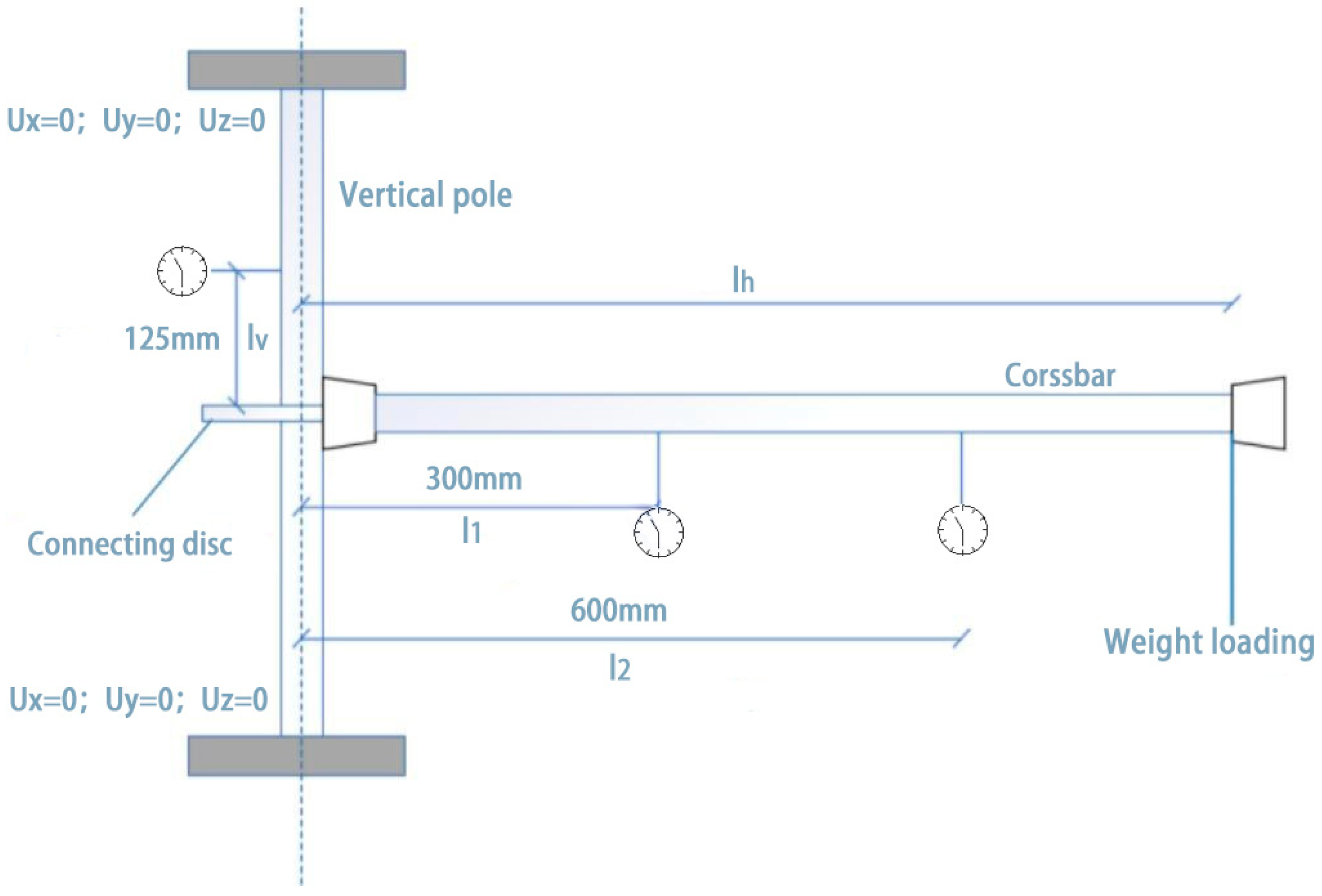
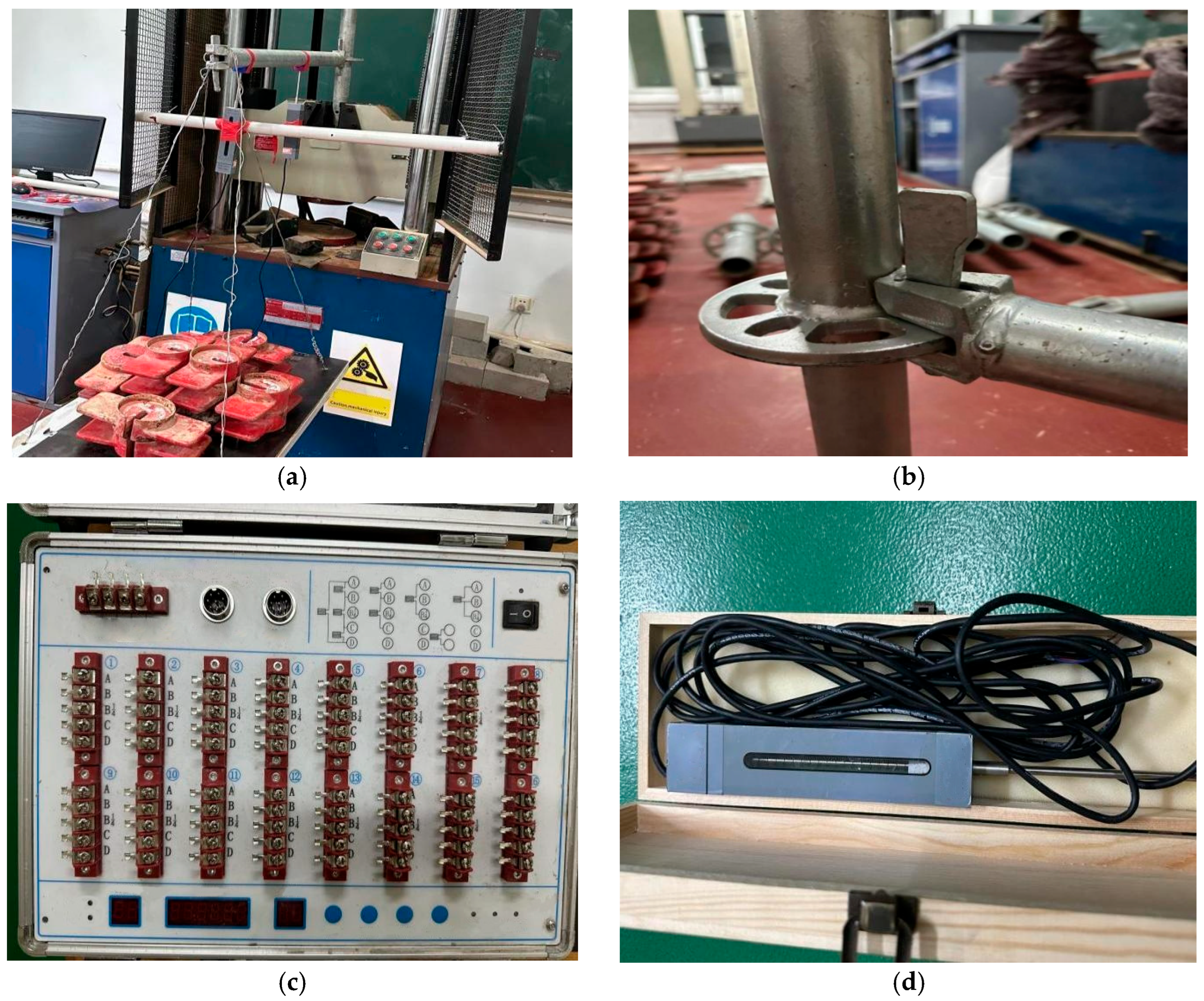
2.2. Test Scheme

The bending stiffness test was conducted using a $\Phi$48-type disc-buckle component. The vertical pole was secured to a universal testing machine, establishing fixed connection boundary conditions at both ends. Horizontal bars were positioned at distances of 300 mm and 600 mm from the axis of the vertical bar. Displacement meters were installed at the upper end of the vertical bar, positioned 125 mm vertically from the horizontal bar axis to ensure precise displacement measurements. Prior to initiating the formal test, pre-loading procedures were implemented. Displacement meter readings were recorded after the vertical rod and the horizontal rods were securely fixed. Testing commenced only after the displayed values stabilized and proper functioning of all measurement devices was confirmed. The formal loading protocol involved the incremental application of weights at the free end of the crossbar, with uniform 100 N increments at each loading stage. After each increment, measurements were recorded only after monitoring data had fully stabilized, and the change values of YWD displacement meter were captured using a uT7116 high-speed static strain gauge. The displacement meter values were continuously monitored until no further changes were observed, at which point the loading process was terminated. The average rotation angle data was subsequently calculated and adopted as the definitive test result. Galvanized steel pipes were utilized throughout this experimental investigation. To prevent potential slippage of the displacement meters during operation, round covers were affixed at the contact points between the displacement meters and the horizontal bar, thereby ensuring stability and maintaining data accuracy throughout the testing procedure.

The experimental investigation utilized six sets of disc-type steel pipe members, which were randomly selected from the construction site. For each assembly, the connection between the horizontal and vertical bars was secured by completely wedging the bolt using a hammer, thereby establishing consistent joint conditions across all test specimens. The test schematic representation of the testing configurations is illustrated in Figure 1. The detailed specifications and material properties of the testing components and instrumentation are presented in

Table 1. Test component specifications and materials.

Component Name	Upright Stanchion	Crossbar	Connecting Disc	Bolt
Specification/mm	$\Phi$48 × 3.2	$\Phi$48 × 2.5	130 × 10	5
material quality	Q345A	Q235B	Q235B	Q235B

. Figure 2 provides a photographic documentation of the actual joint bending test during execution.

2.3. Test Model

During the test, respective displacements were generated in both horizontal and vertical bars. These displacement measurements were subsequently converted into relative rotation angles between the horizontal and vertical bars following load application:

$$\theta ={\displaystyle \frac{1}{2}}\sum _{\mathrm{i}=1}^{\mathrm{n}=2}[{\tan }^{-1}{\displaystyle \frac{{∆}_i}{{\mathrm{l}}_{\mathrm{i}}}}-{\tan }^{-1}{\displaystyle \frac{{∆}_v}{{\mathrm{l}}_{\mathrm{v}}}}]$$

(1)

In the formula, the following symbols are used:

• ${∆}_i$—The displacement value generated by the bar;
• ${∆}_v$—The horizontal displacement value of the pole;
• ${\mathrm{l}}_{\mathrm{v}}$—The vertical distance from the measuring point on the vertical bar to the axis of the horizontal bar;
• ${\mathrm{l}}_{\mathrm{i}}$—The horizontal distance from the measuring point on the vertical bar to the measuring point on the horizontal bar.

Under vertical concentrated loading conditions, the bending moment and corresponding bending stiffness of the plate buckle joint were determined using the following relationship:

$$\mathrm{k}={\displaystyle \frac{M}{\theta }}=2F{\mathrm{l}}_{\mathrm{h}}/\sum _{\mathrm{i}=1}^{\mathrm{n}=2}\left[{\tan }^{-1}{\displaystyle \frac{{∆}_i}{{\mathrm{l}}_{\mathrm{i}}}}-{\tan }^{-1}{\displaystyle \frac{{∆}_v}{{\mathrm{l}}_{\mathrm{v}}}}\right]$$

(2)

In the formula, the following symbols are used:

• ${\mathrm{l}}_{\mathrm{h}}$—The horizontal distance between the action point of the vertical concentrated force of the horizontal bar and the axis of the vertical bar;
• $F$—The concentrated load applied vertically by the transverse bar;
• $M$—The bending moment of the plate-buckle joint.

The calculation model employed for the joint bending stiffness test is illustrated in Figure 3.

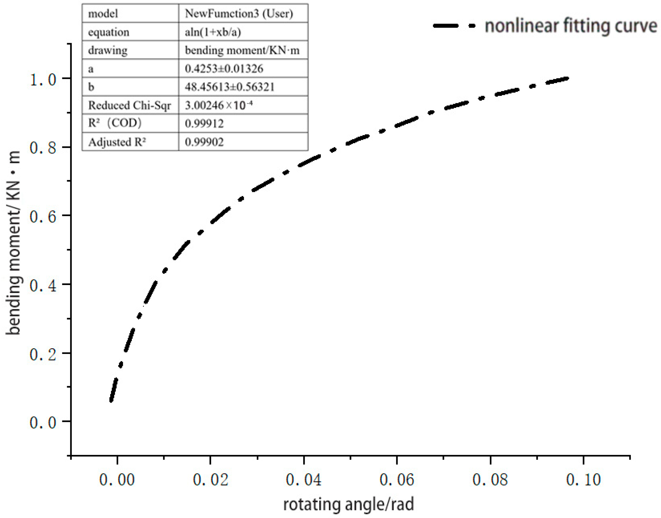
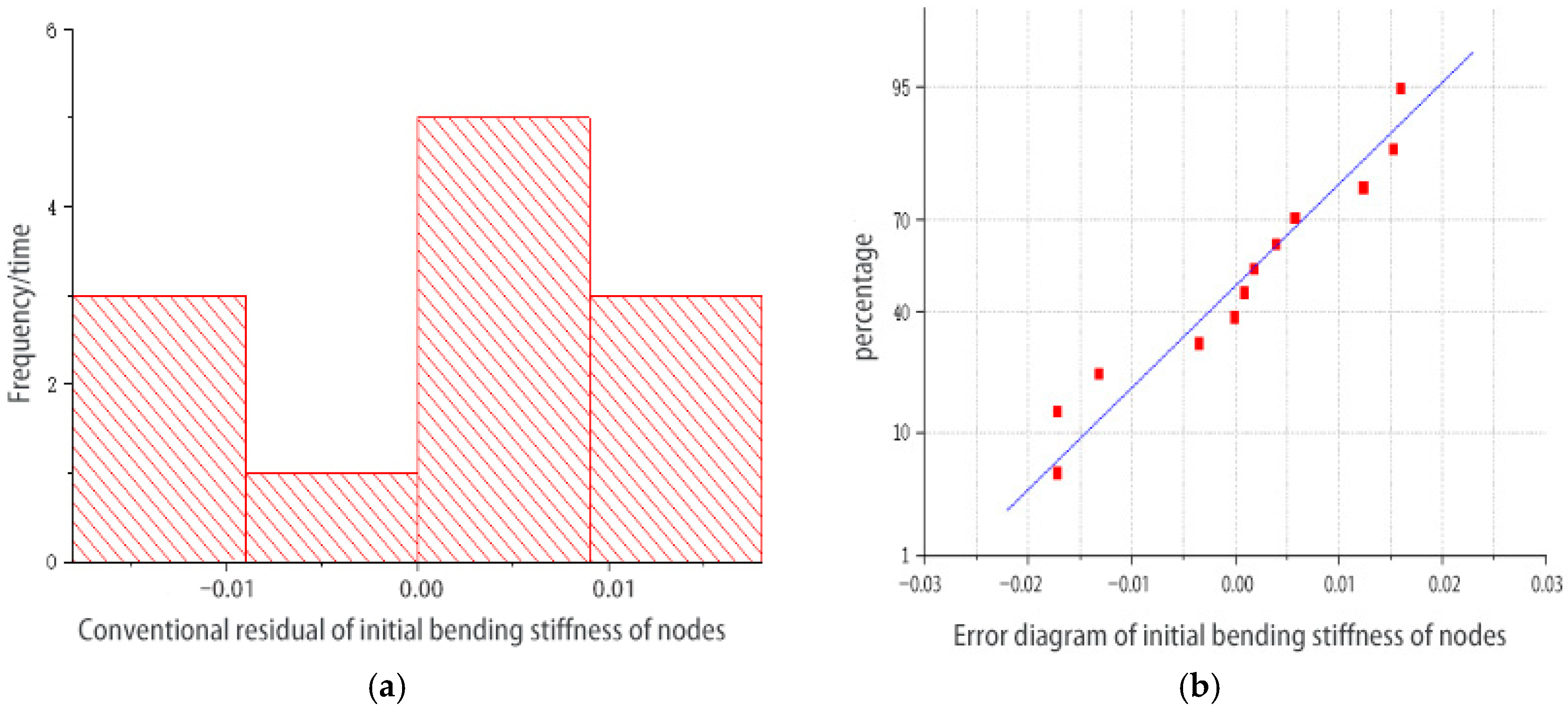
2.4. Experimental Data Processing

The experimental data obtained from joint bending stiffness tests was processed by substituting the measured values into Equation (1) to calculate the relative rotation angles. The relative rotation angles were subsequently imported into specialized graphical analysis software to generate scatter plots representing the relationship between bending moments and rotational deformation. Nonlinear regression analysis was then performed on these data points to establish the characteristic bending moment–rotation relationship curve for the disc-buckle joint. The resultant curve, which characterizes the semi-rigid behavior of the connection, is presented in Figure 4. In the figure, HG-1 to HG-6 represent the six ledgers of the six groups of rosette-type steel tube specimens, respectively.

As illustrated in Figure 4, a nonlinear relationship can be observed between the bending moment and the rotation angle of the plate-buckle joint. The experimental data reveals that during the initial loading phase, minimal changes occur in the vertical displacement of the transverse bar, resulting in relatively small rotation angles and deformation, while the joint exhibits a higher initial stiffness value. As the joint is progressively subjected to concentrated force, both rotation angle and deformation at the joint gradually increase. The declining slope of the curve in Figure 4 indicates a progressive reduction in joint stiffness. In the limiting state of the joint’s bending stiffness, the curve’s progression noticeably decelerates, the joint stiffness degenerates, and a transformation from rigid connection to semi-rigid connection is observed. Based on the aforementioned curves, a two-parameter logarithmic nonlinear mathematical model was employed using mathematical statistical software to fit the semi-rigid model data of the disc-buckle joints. To accurately determine the initial bending stiffness value of the joints, an average was calculated from the six experimental data sets, yielding an initial bending stiffness value of 48.456 kN·m/rad. The resultant fitting curve is presented in Figure 5.

The fitting function is

$$M=0.4253\ln (1+{\displaystyle \frac{48.456}{0.4253}}\theta )$$

(3)

By calculating the fitted frequency distribution of the six sample groups, a frequency histogram was plotted, as shown in Figure 6.

The initial bending stiffness of joints exhibits some variability due to various factors; however, as shown in Figure 6, the fitted initial bending stiffness demonstrates good agreement with small errors.

3. Finite Element Simulation Analysis

In this study, the finite element model of steel tubular joints was established using ABAQUS 2024 finite element software. Finite element analysis was conducted based on joint test to simulate loading process of joint bending test.

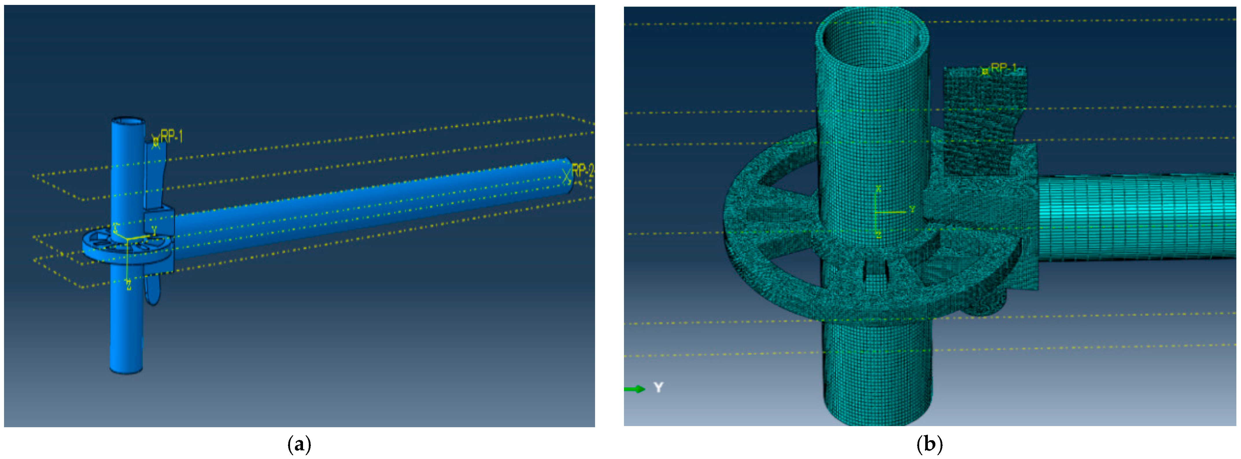
3.1. Finite Element Module Method

(1)

Element Selection

The model was constructed utilizing C3D8 R elements, with solid elements being modeled according to the actual dimensions of the connecting disc, bolt, and lock head.

(2)

Boundary Condition

To replicate the authentic test conditions, both ends of the vertical rod were fixed in the card slot of the universal testing machine. When applying boundary conditions in ABAQUS, the six degrees of freedom at both ends of the vertical rod were constrained to achieve fixed support at both termini. A reference point was established at the loading position of the transverse rod, and the cross section of the transverse rod was coupled and connected. Surface-to-surface contact was implemented between components. The connection relationships between components were simulated by defining tangential friction contact and normal hard contact.

(3)

Constitutive Model

The yield behavior of the steel tube material adheres to the von Mises criterion. In the model, an elastic modulus of $\mathrm{E}=2.06\times {10}^5 \mathrm{M}\mathrm{P}\mathrm{a}$ and a Poisson ‘s ratio of $\mathsf{\mu }=0.3$ were applied. To accurately characterize the plastic region of the material, appropriate conversions were performed through specific formulations based on the actual stress–strain relationship of the material.

The constitutive equation is

$$\sigma =\left\{\begin{array}{c}\mathrm{E}{\mathsf{\epsilon }}_{\mathrm{n}\mathrm{o}\mathrm{m}}\\ {\sigma }_{nom}\ln (1+{\epsilon }_{nom})\end{array}\right.$$

(4)

In the formula, the following symbols are used:

• $\mathrm{E}$—Elastic modulus;
• ${\epsilon }_{nom}$—True strain;
• ${\sigma }_{nom}$—True stress.

(4)

Model Building

After creating the individual components of the rosette joint, the assembly was performed, and meshing was applied to the upright, ledger, connecting rosette, pin, and locking head to establish a refined finite element model. During this process, a mesh size of 3.5 mm was uniformly assigned to all components to ensure the accuracy of the analysis results.

To further verify the stability of the simulation results, a mesh sensitivity analysis was conducted. The model was meshed with three different element sizes (5 mm, 10 mm, and 15 mm), and the moment–rotation relationship at the joint was calculated for each. The results indicated that reducing the mesh size from 15 mm to 10 mm caused significant changes in the moment–rotation curve, whereas further reduction from 10 mm to 3.5 mm resulted in less than 1% variation. Therefore, to balance computational accuracy and efficiency, a mesh size of 3.5 mm was selected for the finite element modeling in this study.

To achieve a more accurate simulation of the structural response, ten analysis steps were established, with each step corresponding to a specific loading level, which represents the incremental loading process in the finite element simulation. Upon submission of the model, static finite element analysis was conducted. The finite element model is illustrated in Figure 7.

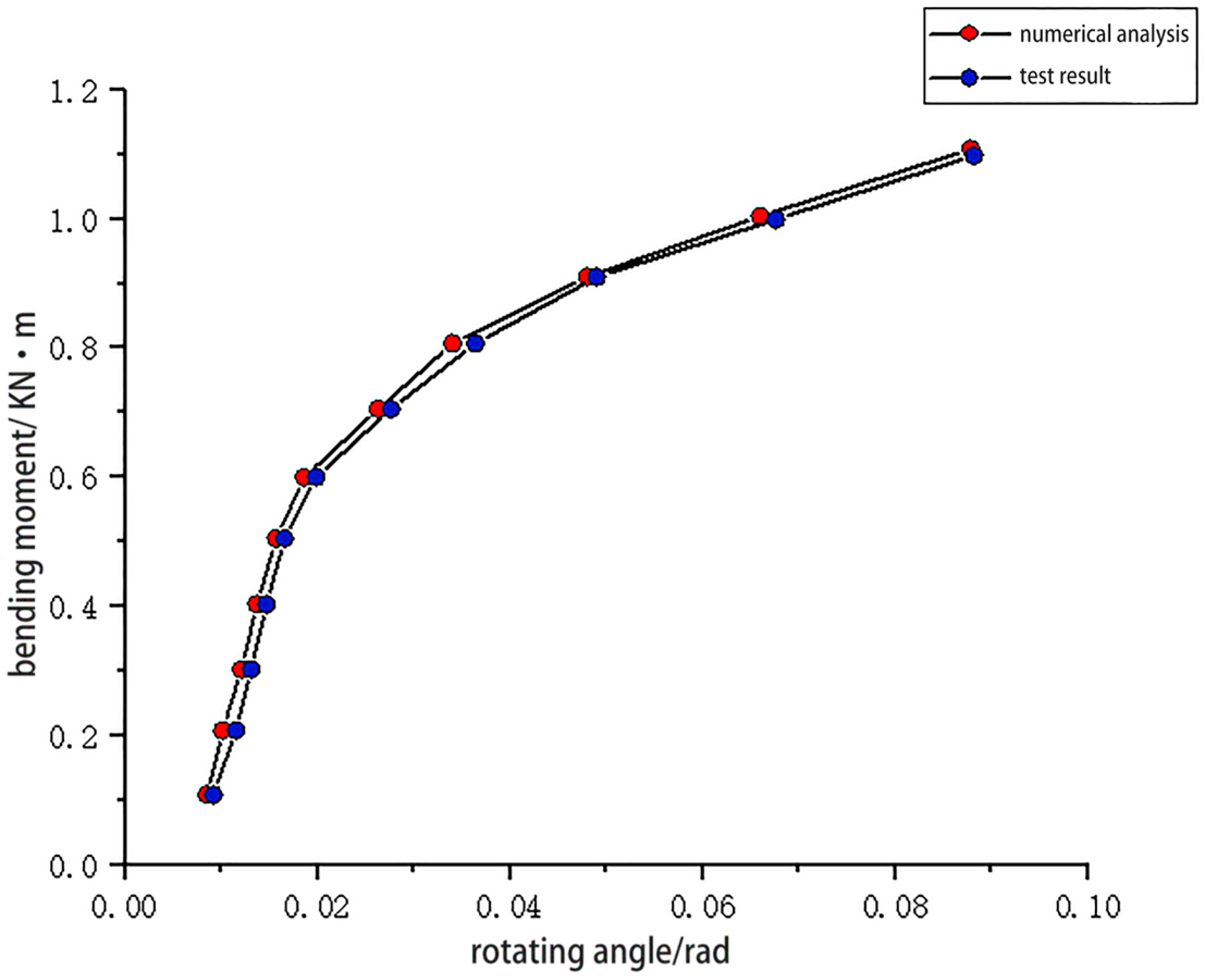
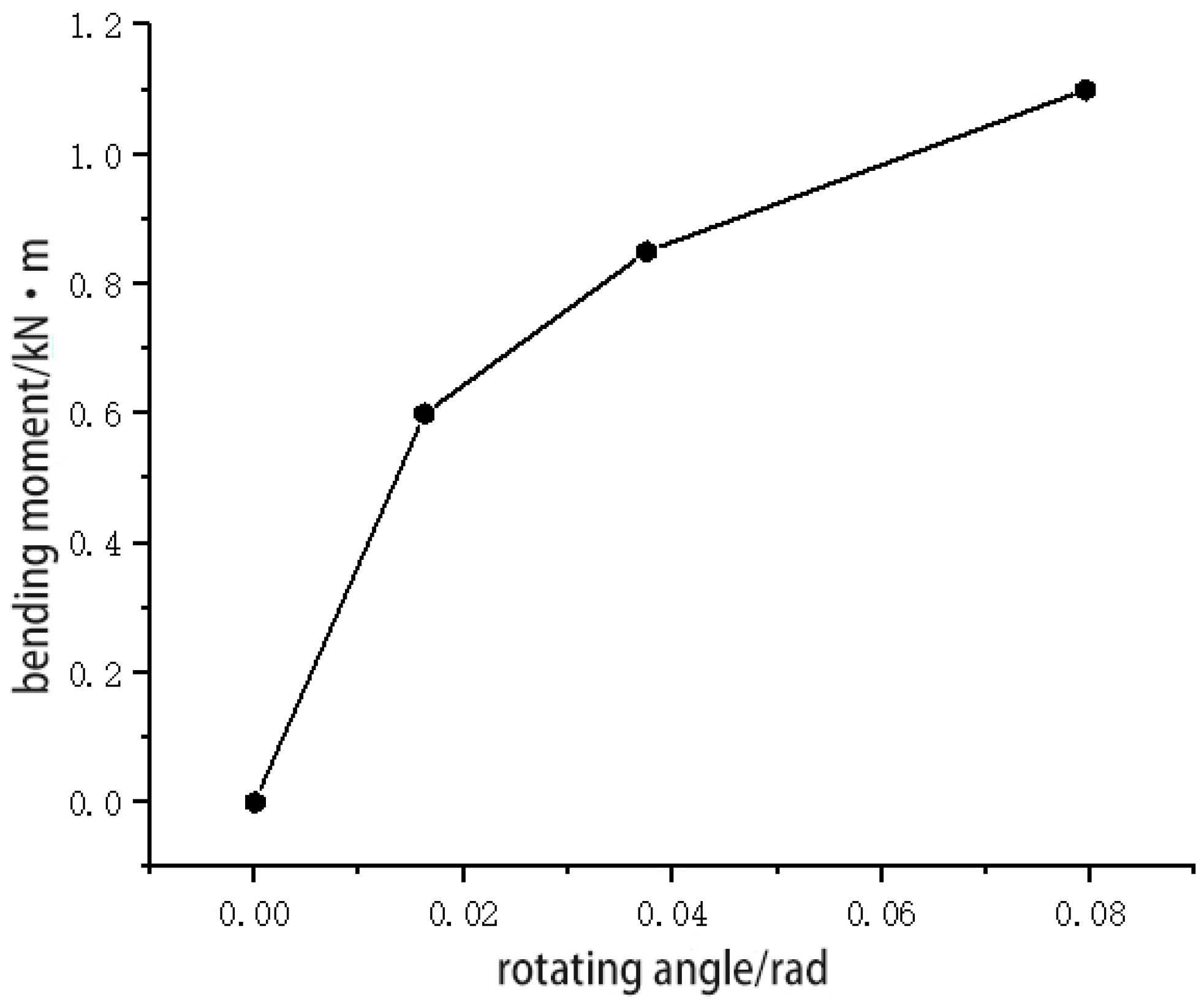
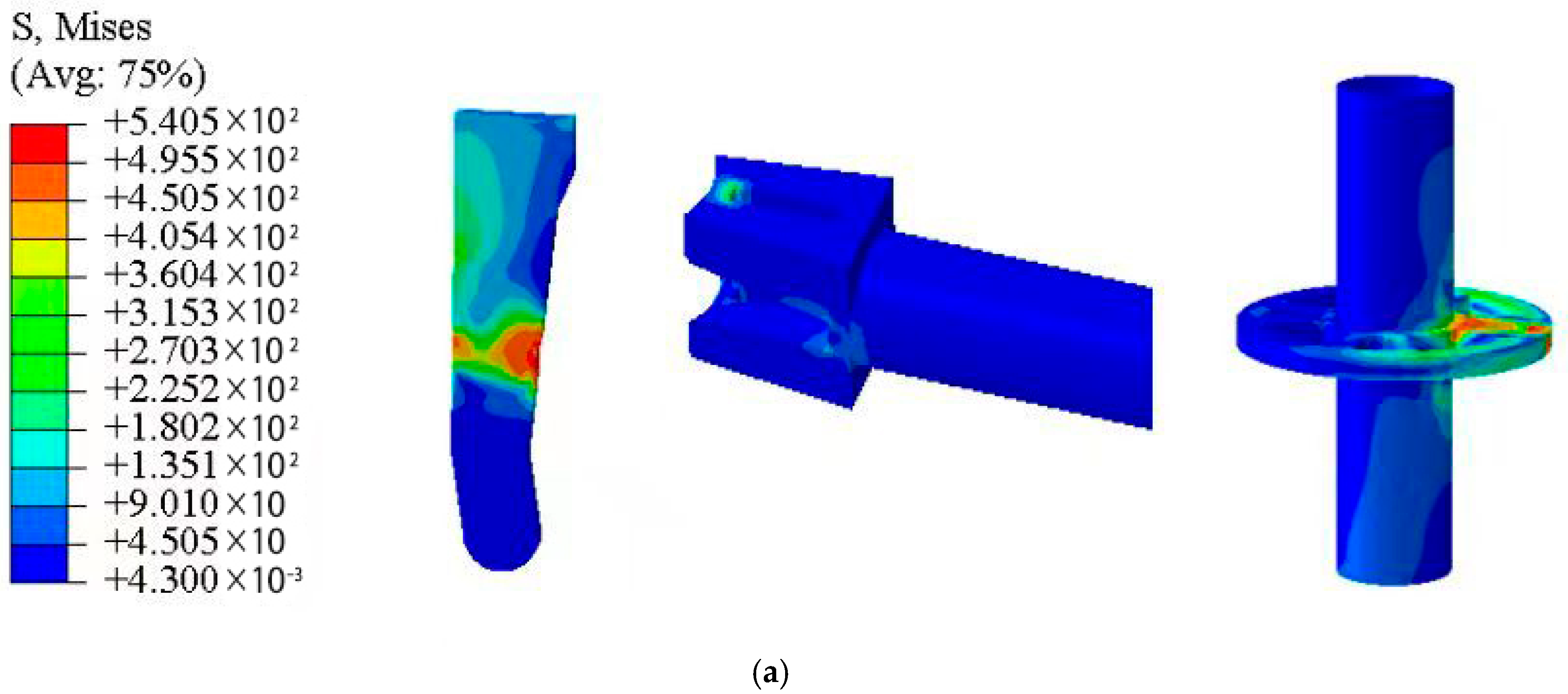
3.2. Numerical Simulation Results

Based on the model wherein the pin was fixed in position, gravity was applied to the end of the crossbar, and the test load was subsequently applied to the extremity of the crossbar at the maximum distance from the vertical bar, following the loading protocol specified in the experiment. Upon completion of the finite element numerical simulation, analysis of the simulation results revealed three distinct stages of joint force behavior. The moment–rotation angle values of the joint under loading conditions were obtained, and subsequently plotted into a moment–rotation angle comparison diagram of the joint, as illustrated in Figure 8.

During the loading process, the buckle joint undergoes a transition from elasticity to elastoplasticity, exhibiting significant nonlinear characteristics in its bending stiffness throughout this transformation [20]. When the joint moment is less than 600 N·m, the moment–rotation curve of the rosette joint can be approximated as a straight line. At this initial loading stage, the joint stiffness remains nearly constant, indicating that the rosette joint is assumed to be in the elastic phase. When the moment is between 600 N·m and 800 N·m, an inflection point appears on the bending curve, and the bending stiffness decreases, indicating the joint has entered the elastic–plastic stage. When the moment exceeds 800 N·m, the slope of the curve decreases again, reflecting a further reduction in stiffness due to the progressive expansion of the plastic zone within the rosette joint. Between 800 N·m and 1100 N·m, the moment–rotation curve gradually converges, suggesting that the joint has entered the plastic deformation development stage.

In summary, this paper proposes a three-stage function of the bending stiffness value of the disc-buckled joint based on test and numerical simulation.

$$\mathrm{M}=\left\{\begin{array}{c}34.423\mathsf{\theta }(0\le \mathrm{M}\le 0.6\mathrm{k}\mathrm{N}·\mathrm{m})\\ 0.3867+12.2387\mathsf{\theta }(0.6\mathrm{k}\mathrm{N}·\mathrm{m}\le \mathrm{M}\le 0.8\mathrm{k}\mathrm{N}·\mathrm{m})\\ 2.4736+5.4576\mathsf{\theta }(0.8\mathrm{k}\mathrm{N}·\mathrm{m}\le \mathrm{M}\le 1.1\mathrm{k}\mathrm{N}·\mathrm{m})\end{array}\right.$$

(5)

The moment–rotation trilinear diagram of the joint is shown in Figure 9:

When the bending moment of the joint is below 600 N·m, the bending moment–rotation curve of the disc-buckle joint can be approximated as linear. At this stage, the stiffness value of the joint remains virtually constant during the initial loading phase, and the disc-buckle joint is considered to be in the elastic stage. When the bending moment ranges between 600 N·m and 800 N·m, an inflection point is observed in the joint’s bending $M$–$\theta$ curve. During this phase, the bending stiffness of the joint decreases, indicating the joint’s transition into the elastoplastic stage. When the joint’s bending moment exceeds 800 N·m, the curve’s slope exhibits a further decrease, demonstrating an additional reduction in the stiffness value of the disc-buckle joint. This phenomenon can be attributed to the progressive expansion of the plastic zone within the disc-buckle joint. As the bending moment increases beyond 800 N·m but remains below 1100 N·m, the $M$–$\theta$ curve of the joint gradually converges, signifying the joint’s entry into the plastic development stage. The stress distribution across these three stages is illustrated in Figure 10.

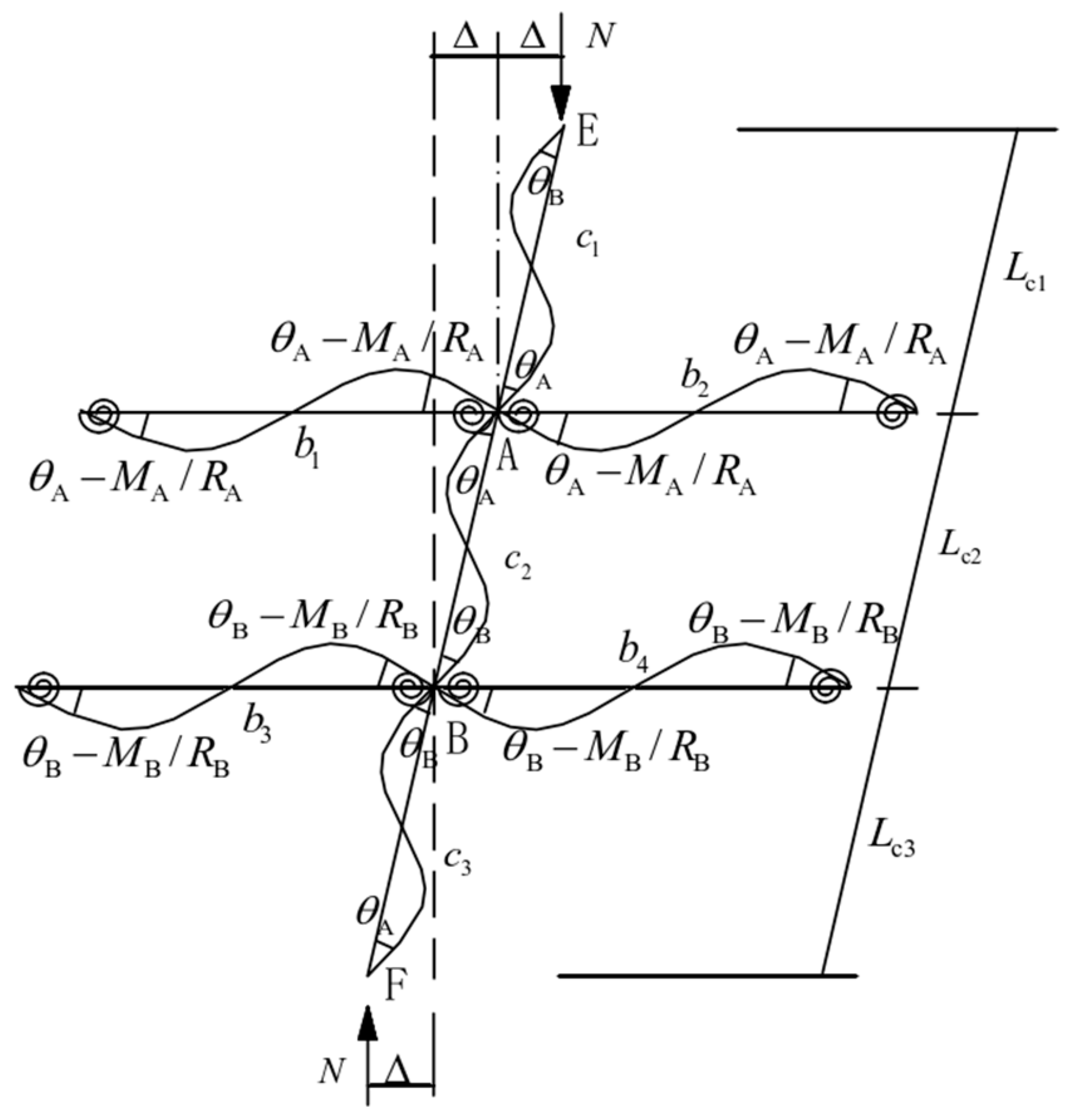
4. Derivation of Effective Length Correction Coefficient Based on Semi-Rigid Joint

Reference [10] considered the influence of the nonlinear moment–rotation relationship of the joint, the constraint of the beam, and the different constraints on the effective length coefficient of the column. By modeling the frame column, the calculation formula of the effective length coefficient of the semi-rigid connection frame column was successfully derived. This method can more accurately reflect the actual stress state of the structure and provide a more accurate basis for structural design. As shown in Figure 11, the three-story frame column model with lateral displacement is shown.

$$\left[36{\mathrm{K}}_1{\mathrm{K}}_2-{\left({\displaystyle \frac{\mathsf{\pi }}{\mathrm{\mu }}}\right)}^2\right]\mathrm{t}\mathrm{a}\mathrm{n}{\displaystyle \frac{\mathsf{\pi }}{\mathrm{\mu }}}+6\left({\mathrm{K}}_1+{\mathrm{K}}_2\right){\displaystyle \frac{\mathsf{\pi }}{\mathrm{\mu }}}$$

(6)

When the connection mode of the two ends of the beam is semi-rigid connection, the bending moment equation of the beam end is

$$M_1={\displaystyle \frac{\mathrm{E}{\mathrm{I}}_{\mathrm{b}}}{{\mathrm{L}}_{\mathrm{b}}}}\left[4\left({\theta }_1-{\displaystyle \frac{M_1}{R_{K_1}}}\right)+2\left({\theta }_2-{\displaystyle \frac{M_2}{R_{K_2}}}\right)\right]$$

(7)

$$M_2={\displaystyle \frac{\mathrm{E}{\mathrm{I}}_{\mathrm{b}}}{{\mathrm{L}}_{\mathrm{b}}}}\left[4\left({\theta }_1-{\displaystyle \frac{M_1}{R_{K_1}}}\right)+4\left({\theta }_2-{\displaystyle \frac{M_2}{R_{K_2}}}\right)\right]$$

(8)

In the formula, the following symbols are used:

• $\mathrm{E}{\mathrm{I}}_{\mathrm{b}}$—Bending stiffness of the horizontal bar;
• $R$—Bending stiffness of disc-buckle joints;
• ${\mathrm{L}}_{\mathrm{b}}$—Horizontal and vertical distance.

When considering the effective length coefficient of the frame column, it is necessary to pay attention to the constraint condition of the beam end, because the stiffness of the constraint condition plays a decisive role in the determination of the coefficient. The stiffness of this constraint condition is achieved by adjusting the stiffness at both ends of the beam. Therefore, when analyzing the frame structure, it is very important to accurately adjust the stiffness value of the beam end for fully paying attention to the semi-rigid properties of the joints. In order to facilitate the calculation, the effective length coefficient μ of the frame column with lateral displacement can be solved by the simplified formula in the ‘Steel Structure Design Standard’ [8]:

$$\mathsf{\mu }=\sqrt{\frac{7.5{\mathrm{K}}_1{\mathrm{K}}_2+4{\mathrm{K}}_1{\mathrm{K}}_2+1.52}{7.5{\mathrm{K}}_1{\mathrm{K}}_2+{\mathrm{K}}_1{\mathrm{K}}_2}}$$

(9)

This paper focuses on the theoretical analysis of semi-rigid connection frame columns subjected to lateral displacement, with particular emphasis on the relationship between the effective length coefficient and the constraint coefficients at the upper and lower ends of the column. In analyzing this frame configuration, accurate determination of the effective length coefficient is crucial, considering both the lateral displacement characteristics of the structure and the semi-rigid characteristics of the connecting nodes. Consequently, when accounting for the semi-rigid characteristics of the joint, it is necessary to modify the stiffness at the ends of the transverse bars in the disc-buckle steel pipe support. The derivation of the effective length coefficient for the neutral rod of the disc-buckle steel pipe support requires simplification based on the following assumptions:

(1)

The rods consist of elastic members with uniform cross sections;

(2)

The axial force in the crossbar is negligibly small;

(3)

The rotation angles at both ends of the crossbar are equal meaning that the rotational stiffness values at both ends are identical (${\mathrm{R}}_{\mathrm{K}1}={\mathrm{R}}_{\mathrm{k}2}$), and correspond to the rotational stiffness value of the plate buckle joint;

(4)

During the frame buckling process, both ends of the crossbar exhibit identical degrees of rotation in the same direction;

(5)

The connection nodes demonstrate semi-rigid behavior;

(6)

When buckling occurs, the moment generated at the joint by the end of the vertical bar is distributed according to the linear stiffness of the transverse bar to achieve equilibrium.

Substitute the above assumptions into Formulas (7) and (8), and obtain Formula (10):

$$M_1={\displaystyle \frac{6\mathrm{E}{\mathrm{I}}_{\mathrm{b}}}{{\mathrm{L}}_{\mathrm{b}}}}·{\theta }_1·{\displaystyle \frac{1}{1+6\mathrm{E}{\mathrm{I}}_{\mathrm{b}}/{\mathrm{L}}_{\mathrm{b}}R}}$$

(10)

The analysis reveals that the correction coefficient of the bar line stiffness is

$$\mathsf{\alpha }={\displaystyle \frac{1}{1+6\mathrm{E}{\mathrm{I}}_{\mathrm{b}}/{\mathrm{L}}_{\mathrm{b}}R}}$$

(11)

In the formula, the following symbols are used:

• ${\mathrm{L}}_{\mathrm{b}}$—Horizontal and vertical distance;
• $R$—Bending stiffness of disc-buckle joints;
• ${\mathrm{I}}_{\mathrm{b}}$—Moment of inertia of the cross section of the bar;
• $\mathrm{E}$—Elastic modulus of the bar.

Furthermore, the effective length coefficient μ of the frame column with lateral semi-rigid connection is derived as

$$\mathsf{\mu }=\sqrt{{\displaystyle \frac{7.5\alpha k_1{k}_2+4\left(\alpha k_1\alpha k_2\right)+1.52}{7.5\alpha k_1\alpha k_2+\alpha k_1+\alpha k_2}}}$$

(12)

Of which

$$k_1={\displaystyle \frac{{\mathrm{I}}_{\mathrm{b}1}/{\mathrm{L}}_{\mathrm{b}1}{+\mathrm{I}}_{\mathrm{b}2}/{\mathrm{L}}_{\mathrm{b}2}}{{\mathrm{I}}_{\mathrm{c}1}/{\mathrm{L}}_{\mathrm{c}1}{+\mathrm{I}}_{\mathrm{c}2}/{\mathrm{L}}_{\mathrm{c}2}}}$$

(13)

$$k_2={\displaystyle \frac{{\mathrm{I}}_{\mathrm{b}3}/{\mathrm{L}}_{\mathrm{b}3}{+\mathrm{I}}_{\mathrm{b}4}/{\mathrm{L}}_{\mathrm{b}4}}{{\mathrm{I}}_{\mathrm{c}2}/{\mathrm{L}}_{\mathrm{c}2}{+\mathrm{I}}_{\mathrm{c}3}/{\mathrm{L}}_{\mathrm{c}3}}}$$

(14)

In these equations, the following symbols are used:

• $k_1$—The ratio of the sum of the linear stiffness of the upper part of the horizontal bar to the sum of the linear stiffness of the vertical bar;
• $k_2$—The ratio of the sum of the linear stiffness of the lower part of the horizontal bar to the sum of the linear stiffness of the vertical bar.

According to the ‘Safety Technical Specification for Construction Plug-and-Plug Disc Buckle Steel Pipe Brackets JGJ231-2010’ [21], the specifications and section characteristics of the vertical and horizontal rods are provided in

Table 2. Specifications and cross-section characteristics of vertical and horizontal rods.

Type	Specification/mm	Length/m	Sectional Moment of Inertia/m4	Elastic Modulus/kN·m2
Pillars	$\Phi 48\times 3.2$	0.5, 1.0, 1.5, 2.0	11.36 × 10−8	2.06 × 10−8
	$\Phi 48\times 2.5$	0.3, 0.6, 0.9, 1.2, 1.5, 1.8	9.28 × 10−8	2.06 × 10−8
Crossbar	$\Phi 48\times 3.2$	0.5, 1.0, 1.5, 2.0	11.36 × 10−8	2.06 × 10−8
	$\Phi 48\times 2.5$	0.3, 0.6, 0.9, 1.2, 1.5, 1.8	9.28 × 10−8	2.06 × 10−8

.

Let $\mathrm{K}=\mathsf{\alpha }\mathrm{k}$,

$$\mathrm{K}={\displaystyle \frac{{\mathrm{I}}_{\mathrm{b}}}{{\mathrm{I}}_{\mathrm{c}}}}\times {\displaystyle \frac{{\mathrm{L}}_{\mathrm{c}}R}{{\mathrm{L}}_{\mathrm{b}}R+6\mathrm{E}{\mathrm{I}}_{\mathrm{b}}}}$$

(15)

The above formula demonstrates that the calculation length correction coefficient $\mu$ is primarily dependent on the joint’s bending stiffness, the transverse and longitudinal spacing of the vertical bar, and the step distance. Based on the experimental results previously obtained, the initial bending stiffness of the joint ranges from 7.914 kN·m/rad to 48.456 kN·m/rad. For this analysis, a conservative bending stiffness value of R = 24 kN·m/rad has been adopted, yielding the revised effective length coefficient ${\mathsf{\mu }}_0$ as presented in

Table 3. Calculated length correction factors.

Working Condition	Step/m	Horizontal and Vertical Distance/m	Correction Factor/${\mathit{\mu }}_{\mathbf{0}}$
1	0.5	0.3	1.7015
2	0.5	0.6	1.7419
3	0.5	0.9	1.7836
4	0.5	1.2	1.8153
5	0.5	1.5	1.8471
6	0.5	1.8	1.8859
7	1.0	0.3	1.2779
8	1.0	0.6	1.3388
9	1.0	0.9	1.3982
10	1.0	1.2	1.4561
11	1.0	1.5	1.5127
12	1.0	1.8	1.5680
13	1.5	0.3	1.2653
14	1.5	0.6	1.2876
15	1.5	0.9	1.3017
16	1.5	1.2	1.3212
17	1.5	1.5	1.3514
18	1.5	1.8	1.3790
19	2.0	0.3	1.0078
20	2.0	0.6	1.1102
21	2.0	0.9	1.1497
22	2.0	1.2	1.1733
23	2.0	1.5	1.1950
24	2.0	1.8	1.2179

.

5. Engineering Example

5.1. Project Profile

To validate the engineering applicability of the calculated length correction coefficient proposed in this paper, an expansion terminal project at an airport in Xi’an, Shaanxi Province was selected as a case study, with specific focus on the east side corridor area. The structural configuration of this area is a frame structure, which is differentiated into structural plate and non-structural plate zones. In the structural plate zone, the frame is erected directly on the structural plate, whereas in the non-structural plate zone, the frame is installed on a cushion foundation, which is underlain by a 500 mm thick lime soil cushion and 3–4 m plain soil compaction piles. For stability assessment purposes, this analysis examines the highest support frame deployed in the project, which has a height of 12 m, a maximum floor thickness of 180 mm, and both longitudinal and transverse dimensions of 20 m.

5.2. Design Scheme of Disc-Buckle Steel Pipe Support

(1)

The disc-type steel pipe support has a height of 12 m and a span of 20 m.

(2)

Support frame dimensional specifications: pole step distance h = 1.5 m, pole vertical distance (span direction) L = 1.2 m, horizontal distance 1.2 m, top extension height a = 0.5 m.

(3)

Permanent load of support:

The standard value of the weight of the template is usually 0.5 kN/m², and the standard value of the weight of the support q is 0.15 kN/m; then,

$${\mathrm{G}}_{1\mathrm{k}}=0.15\times 12.3+0.5\times 1.2\times 1.2=2.565 \mathrm{k}\mathrm{N}$$

The standard value of concrete weight is 24 kN/m³; then,

$${\mathrm{G}}_{2\mathrm{k}}=24\times 0.18\times 1.2\times 1.2=6.2208 \mathrm{k}\mathrm{N}$$

The standard value of steel bar weight is 1.1 kN/m³; then,

$${\mathrm{G}}_{3\mathrm{k}}=1.1\times 0.18\times 1.2\times 1.2=0.28512 \mathrm{k}\mathrm{N}$$

Therefore, the bracket permanent load is

$$\sum {\mathrm{N}}_{\mathrm{G}\mathrm{K}}={\mathrm{G}}_1+{\mathrm{G}}_2+{\mathrm{G}}_3=9.071 \mathrm{k}\mathrm{N}$$

(4)

Bracket variable load:

The standard value of load generated by on-site construction personnel and their equipment is usually taken as 3 kN/m²; then,

$${\mathrm{Q}}_{1\mathrm{k}}=3\times 1.2\times 1.2=4.32 \mathrm{k}\mathrm{N}$$

When determining the standard value of horizontal load, it is usually set to 2% of the standard value of permanent load by referring to the actual effects of activities such as pumping and dumping concrete. This kind of load mainly acts on the most unfavorable position in the upper part of the structure, which has a non-negligible impact on the overall stability of the structure; then,

$${\mathrm{Q}}_{2\mathrm{k}}=0.02\times \sum {\mathrm{N}}_{\mathrm{G}\mathrm{K}}=0.1814 \mathrm{k}\mathrm{N}$$

Therefore, the bracket variable load is

$$\sum {\mathrm{Q}}_{\mathrm{G}\mathrm{K}}={\mathrm{Q}}_1+{\mathrm{Q}}_2=4.5014 \mathrm{k}\mathrm{N}$$

(5)

Wind load parameters: The basic wind pressure is ${\mathsf{\omega }}_0$= 0.25 kN/m², the ground roughness is B (urban suburbs), the height variation coefficient of wind pressure is ${\mathsf{\mu }}_{\mathrm{z}}$= 1.06, and the shape coefficient of wind load is ${\mathsf{\mu }}_{\mathrm{s}}$ = 0.5. The standard value of wind load is calculated as follows:

$${\mathsf{\omega }}_{\mathrm{k}}={\mathsf{\omega }}_0{\mathsf{\mu }}_{\mathrm{z}}{\mathsf{\mu }}_{\mathrm{s}}=0.25\times 1.06\times 0.5=0.133 \mathrm{k}\mathrm{N}·{\mathrm{m}}^2$$

According to Formula in the ‘Technical Standard for Safety of Plug-in Disc-type Steel Pipe Scaffolding in Building Construction’, the wind load should be considered when evaluating the stability of the vertical bar, with a combination coefficient of 0.9 under these conditions.

The calculation formula of wind load ${\mathrm{M}}_{\mathrm{w}}$ design value is

$${\mathrm{M}}_{\mathrm{w}}=0.9{\mathsf{\gamma }}_0{\mathsf{\gamma }}_{\mathrm{Q}}{\mathsf{\gamma }}_{\mathrm{L}}{\mathsf{\omega }}_{\mathrm{k}}{\mathrm{l}}_{\mathrm{a}}{h}^2/10$$

(16)

In the formula, the following symbols are used:

• ${\mathsf{\gamma }}_0$—Structure importance coefficient, 1.1;
• ${\mathsf{\gamma }}_{\mathrm{Q}}$—Variable load partial coefficient, 1.5;
• ${\mathsf{\gamma }}_{\mathrm{L}}$—Variable load adjustment coefficient, 0.9;
• ${\mathsf{\omega }}_{\mathrm{k}}$—Standard value of wind load, calculated 0.133 kN/m²;
• ${\mathrm{l}}_{\mathrm{a}}$—Vertical rod length (m), 1.8 m;
• $\mathrm{h}$—Step distance (m), 1.5 m.

The wind load design value is

$${\mathrm{M}}_{\mathrm{w}}={\displaystyle \frac{0.9{\mathsf{\gamma }}_0{\mathsf{\gamma }}_{\mathrm{Q}}{\mathsf{\gamma }}_{\mathrm{L}}{\mathsf{\omega }}_{\mathrm{k}}{\mathrm{l}}_{\mathrm{a}}{h}^2}{10}}=0.9\times 1.1\times 1.5\times 0.9\times 0.133\times 1.8\times {\displaystyle \frac{{1.5}^2}{10}}=0.072 \mathrm{k}\mathrm{N}·\mathrm{m}$$

5.3. Stability Verification Calculation of Disc-Buckle Steel Pipe Support

The effective length correction coefficient is calculated according to a modified effective length coefficient value from Table 3, utilizing ${\mu }_0$ = 1.3212. For comparison, according to Schedule E.0.2 of the ‘Steel Structure Design Standard’, $\mu$ = 1.24

Slenderness Ratio Verification:

Using the standard $\mu$ value, $l_0={\beta }_H\mu h=1.24\times 1.05\times 1500=1953 \mathrm{mm}$

$$\mathsf{\lambda }=l_0/\mathrm{i}=1953/15.9=123\le \left[\lambda \right]=150$$

$${\mathsf{\lambda }}_{01}=l_{01}/\mathrm{i}=2080.89/15.9=133\le \left[\lambda \right]=150$$

Both values satisfy the requirements.

The percentage difference between the standard value and the modified value is

$${\displaystyle \frac{{\mathsf{\lambda }}_{01}-{\mathsf{\lambda }}_0}{{\mathsf{\lambda }}_0}}={\displaystyle \frac{133-123}{123}}\times 100\%=8.13\%$$

This analysis demonstrates that the slenderness ratio obtained using the effective length coefficient specified by the standard is 8.13% lower than that obtained using the modified effective length coefficient. The reason is that the value of the effective length coefficient specified in the specification has not fully considered the constraint effect of the crossbar of the steel pipe support in the actual project, and the joints under the constraint of the crossbar will produce semi-rigid characteristics, resulting in the calculation of the specification. The length coefficient is too small, which is different from the actual engineering situation. However, the increase in the slenderness ratio makes the members more prone to buckling instability under the same load, thus reducing the safety margin of the structure. The failure mode of the support will also change with the increase in the slenderness ratio, from local buckling to overall buckling, resulting in the transfer of the failure position from the local node to the overall component, which will directly affect the failure process and energy release path of the support. Therefore, the calculated length coefficient in the specification is not safe, and the application will produce non-negligible differences. Based on comprehensive consideration, it is recommended to utilize the modified effective length coefficient that accounts for crossbar constraints when verifying the slenderness ratio.

According to Schedule D-2 of the ‘Technical Specification for Safety of Plug-and-Plug Steel Tubular Scaffolds for Construction’, it can be obtained that $\mathsf{\phi }=0.296$.

(1)

Without Wind Load Consideration:

Design value of vertical rod axial force:

$$\begin{gathered} \mathrm{N}={\mathsf{\gamma }}_0\left({\mathsf{\gamma }}_{\mathrm{G}}\sum {\mathrm{N}}_{\mathrm{G}\mathrm{K}}+{\mathsf{\gamma }}_{\mathrm{Q}}\sum {\mathrm{N}}_{\mathrm{Q}\mathrm{K}}\right)=1.1\times \left(1.3\times 13.3759+1.5\times 4.5014\right)=26.5584 \mathrm{k}\mathrm{N} \\ \mathrm{f}={\displaystyle \frac{\mathrm{N}}{\mathsf{\phi }\mathrm{A}}}={\displaystyle \frac{26558}{0.296\times 453}}=198.064 \mathrm{N}/{\mathrm{m}\mathrm{m}}^2\le \left[\mathrm{f}\right]=300 \mathrm{N}/{\mathrm{m}\mathrm{m}}^2 \end{gathered}$$

This satisfies the requirements.

(2)

With Wind Load Consideration:

Design value of vertical rod axial force:

$$\begin{gathered} {\mathrm{N}}_1=\mathrm{N}+{\mathrm{M}}_{\mathrm{w}}/{\mathrm{l}}_{\mathrm{b}}=26.5584+0.6=27.1584 \mathrm{k}\mathrm{N} \\ {\mathrm{f}}_1={\displaystyle \frac{{\mathrm{N}}_1}{\mathsf{\phi }\mathrm{A}}}+{\displaystyle \frac{{\mathrm{M}}_{\mathrm{w}}}{\mathrm{W}}}={\displaystyle \frac{27158}{0.296\times 453}}+{\displaystyle \frac{7200}{4797}}=204.0386 \mathrm{N}/{\mathrm{m}\mathrm{m}}^2\le \left[\mathrm{f}\right]=300 \mathrm{N}/{\mathrm{m}\mathrm{m}}^2 \end{gathered}$$

This also satisfies the requirements.

In conclusion, the effective length correction coefficient obtained in this paper adequately addresses the requirements for practical engineering calculation.

6. Conclusions

This study presents an analysis of the semi-rigid characteristics of joints and the stability bearing capacity of the disc-type steel pipe supports through experimental testing and numerical simulation. The following conclusions have been drawn:

(1)

The bending stiffness tests of the joints yielded the bending moment–rotation curve for the connection joint of the Φ48-type disc-buckle steel pipe support. Based on these curve characteristics, an appropriate semi-rigid joint calculation model was selected, and nonlinear fitting of the test data was performed. Parametric analysis of the joint’s semi-rigidity determined an initial stiffness value of 48.456 kN·m/rad.

(2)

Finite element analysis was conducted on the Φ48-type disc-buckle steel pipe support joint to simulate the complete process of the joint bending test. Results demonstrate excellent agreement between the finite element simulation of the joint loading process and the experimental data, validating the model’s accuracy. Based on the numerical simulation results, a trilinear fitting function for the $\mathrm{M}$–$\mathsf{\theta }$ relationship curve of the joint flexural member was derived:

$$\mathrm{M}=\left\{\begin{array}{c}34.423\mathsf{\theta }(0\le \mathrm{M}\le 0.6\mathrm{k}\mathrm{N}·\mathrm{m})\\ 0.3867+12.2387\mathsf{\theta }(0.6\mathrm{k}\mathrm{N}·\mathrm{m}\le \mathrm{M}\le 0.8\mathrm{k}\mathrm{N}·\mathrm{m})\\ 2.4736+5.4576\mathsf{\theta }(0.8\mathrm{k}\mathrm{N}·\mathrm{m}\le \mathrm{M}\le 1.1\mathrm{k}\mathrm{N}·\mathrm{m})\end{array}\right.$$

(3)

Utilizing the theory of semi-rigid connection frames with lateral displacement, this study revised the stiffness coefficient $\mathsf{\alpha }$, the constraint coefficient k at the vertical bar end, and the effective length coefficient $\mathsf{\mu }$ of the vertical bar under horizontal bar end constraints, accounting for the joint’s semi-rigidity. For horizontal and vertical bars of varying dimensions, this study established the range and specific values of corresponding effective length correction coefficients for determined construction parameters.

(4)

Using an actual engineering project as a case study, verification of the vertical bar’s slenderness ratio under the calculated length correction coefficient revealed results 8.13% higher than standard specifications. This discrepancy arises because the effective length coefficient specified in the code does not fully account for the semi-rigid characteristics of joints resulting from the constraint effect of the crossbar in steel pipe support in actual projects. Theoretical calculations confirmed that the derived calculation length correction coefficient satisfies practical engineering requirements.

References

- Bing, Z.; Jian, X.; Yan, L. Study on the influence of node stiffness on the dynamic performance of spatial tubular truss arches. Build. Sci. 2022, 38, 16–26. [Google Scholar] [CrossRef]
- Yang, X.; Er, M.; Jing, M. Performance analysis of semi-rigid joints in new steel tube scaffolding. Steel Constr. 2018, 33, 144–149. [Google Scholar] [CrossRef]
- Yan, L.; Mei, R.; Wei, Z. Analysis of the causes of high-formwork collapse accidents based on the “2-4” mod-el. Constr. Saf. 2022, 37, 74–77. [Google Scholar]
- Xin, L.; Wen, L.; Kai, L. Progressive collapse prevention of engineering structures in China: Review and prospect. Build. Struct. 2019, 49, 102–112. [Google Scholar] [CrossRef]
- Chandrangsu, T.; Rasmussen, J.K. Investigation of geometric imperfections and joint stiffness of support scaffold systems. J. Constr. Steel Res. 2010, 67, 576–584. [Google Scholar] [CrossRef]
- ANSI/AISC 360-22; Specification for Structural Steel Buildings. American Institute of Steel Construction—AISC: Chicago, IL, USA, 2022.
- Li, W. Bending buckling of axially compressed members. Build. Struct. 2019, 49, 126–135. [Google Scholar] [CrossRef]
- GB50017-2017; National Standard of the People’s Republic of China. Design Standard for Steel Structure. China Building Industry Press: Beijing, China, 2018.
- Chang, H.; Yan, G.; Yuan, M.; Xiao, B. Experimental study on bearing capacity of formwork support system. J. Xi’an Univ. Archit. Technol. (Nat. Sci. Ed.) 2017, 49, 179–186. [Google Scholar] [CrossRef]
- Jing, W.; Guo, L. Stability analysis of columns in semi-rigidly connected composite frames with lateral displacement. J. Harbin Inst. Technol. 2009, 41, 126–130. [Google Scholar]
- Qing, W.; Ming, S. Lateral displacement mode of column-supported modular steel structures with semi-rigid connections. J. Build. Eng. 2022, 15, 62–64. [Google Scholar] [CrossRef]
- Cimellaro, G.P.; Domaneschi, M.; Cimellaro, P.G.; Domaneschi, M. Stability Analysis of Different Types of Steel Scaffolds. Eng. Struct. 2017, 152, 535–548. [Google Scholar] [CrossRef]
- Cheng, Q.; Kuang, X.; Zong, W.; Li, Q.; Shen, L. Bearing capacity analysis of semi-rigid supports based on energy method. Highway 2021, 66, 193–195. [Google Scholar]
- Blazik-Borowa, E.; Szer, J.; Borowa, A.; Robak, A.; Pienko, M. Modelling of load-displacement curves obtained from scaffold components tests. Bull. Pol. Acad. Sci. Tech. Sci. 2019, 67, 317–327. [Google Scholar] [CrossRef]
- Kong, R.; Lin, F.; Rang, Z.; Wang, Z.; Xu, Z. Study on the stiffness of cuplock nodes in M60 steel tube form-work supports. Ind. Constr. 2023, 1, 1–16. Available online: http://kns.cnki.net/kcms/detail/11.2068.TU.20231020.1036.004.html (accessed on 20 May 2025).
- Xiao, Q. Research on Test and Application Technology of Disc-Buckled and Bowl-Buckled Steel Tube Support Joints. Master’s Thesis, Southeast University, Nanjing, China, 2016. [Google Scholar]
- Guang, C.; Kun, H.; Lei, W.; Ye, C. Investigation of the mechanical properties of inserting-type support frames. Sci. Rep. 2024, 14, 29746. [Google Scholar] [CrossRef]
- Zhao, Z.; Liu, H.; Liang, B. Novel numerical method for the analysis of semi-rigid jointed lattice shell structures considering plasticity. Adv. Eng. Softw. 2017, 114, 208–214. [Google Scholar] [CrossRef]
- Genovese, F.; Sofi, A. A Novel Interval Matrix Stiffness Method for the Analysis of Steel Frames with Uncertain Semi-Rigid Connections. Adv. Eng. Softw. 2024, 192, 103629. [Google Scholar] [CrossRef]
- Gan, S.; Wei, L.; Shao, C. Theoretical research on direct analysis method of semi-rigid steel frames. J. Build. Struct. 2014, 35, 142–150. [Google Scholar] [CrossRef]
- JGJ/T231-2010; Industry Standard of the People’s Republic of China. Technical Code for Safety of Socket Disc Buckle Steel Tube Support in Construction. China Building and Building Press: Beijing, China, 2010.