Article

Wind Tunnel Tests and Buffeting Response Analysis of Concrete-Filled Steel Tubular Arch Ribs During Cantilever Construction

1
School of Civil Engineering, Harbin Institute of Technology, Harbin 150090, China
2
Journal of Building Structures Editorial Office, Beijing 100835, China
*
Author to whom correspondence should be addressed.
Buildings 2025, 15(11), 1837; https://doi.org/10.3390/buildings15111837
Submission received: 16 March 2025 / Revised: 15 May 2025 / Accepted: 20 May 2025 / Published: 27 May 2025
(This article belongs to the Special Issue Research on Concrete Filled Steel Materials in Building Engineering)

Abstract

:
During the construction of concrete-filled steel tubular (CFST) arch bridges, hollow steel tube arch ribs are typically erected using the cantilever method with cable hoisting. In this construction stage, the arch ribs exhibit low out-of-plane stiffness and are thus highly susceptible to wind-induced vibrations, which may lead to cable failure or even collapse of the structure. Despite these critical risks, research on the aerodynamic performance of CFST arch ribs with different cross-sectional forms during cantilever construction remains limited. Most existing studies focus on individual bridge cases rather than generalized aerodynamic behavior. To obtain generalized aerodynamic parameters and buffeting response characteristics applicable to cantilevered CFST arch ribs, this study investigates two common cross-sectional configurations: four-tube trussed and horizontal dumbbell trussed sections. Sectional model wind tunnel tests were conducted to determine the aerodynamic force coefficients and aerodynamic admittance functions (AAFs) of these arch ribs. Comparisons with commonly used empirical AAF formulations (e.g., the Sears function) indicate that these simplified models, or assumptions equating aerodynamic forces with quasi-steady values, are inaccurate for the studied cross-sections. Considering the influence of the curved arch axis on buffeting behavior, a buffeting analysis computational program was developed, incorporating the experimentally derived aerodynamic characteristics. The program was validated against classical theoretical results and practical measurements from an actual bridge project. Using this program, a parametric analysis was conducted to evaluate the effects of equivalent AAF formulations, coherence functions, first-order mode shapes, and the number of structural modes on the buffeting response. The results show that the buffeting response of cantilevered hollow steel arch ribs is predominantly governed by the first-order mode, which can be effectively approximated using a bending-type mode shape expression.

1. Introduction

Concrete-filled steel tubular (CFST) arch bridges have the advantages of high load-bearing capacity, convenient construction, good spanning capacity, and an attractive appearance, which have led to their widespread use globally. In the construction of large-span CFST arch bridges, the cable hoisting method is commonly employed, where hollow arch rib sections are lifted by a cable hoisting system and then cantilevered into position with stay cables. However, during cantilever construction, the hollow arch ribs are solely supported by lateral cables. Due to their low out-of-plane stiffness and inadequate wind resistance, the structure is highly susceptible to stability issues, posing significant safety risks. Field measurements from existing construction projects [1,2] indicate that the cantilevered hollow arch ribs experience severe galloping and buffeting under large wind loads, which can result in large amplitude vibrations and sudden ruptures of both the arch ribs and lateral cables during the construction stage.
To ensure wind-induced vibration stability during cantilever construction, researchers have conducted wind tunnel tests on specific bridges to study their aerodynamic characteristics. Zhou [3] conducted wind tunnel tests on both the deck system section model and the full-bridge aeroelastic model of Yajisha Bridge in China. The results demonstrated that the bridge deck exhibited good wind stability, a high critical flutter wind speed, and no vortex-induced vibrations within the tested wind speed range. Hong [4] conducted wind tunnel tests and buffeting analysis for the Jiantiao Bridge in China, which has a main span of 245 m. The study found that no buffeting instability occurred across various initial wind angles of attack in the bridge deck section model tests. Similarly, Luo [5] investigated buffeting vibrations for a CFST arch bridge with a 344 m span in its final constructed state. A comparison between buffeting analysis results and the average wind response indicated that buffeting vibrations had a negligible impact on the bridge behaviors. Lu [6] investigated the aerodynamic disturbance effects of the main arch ribs of the Nanchang Shengmi Bridge using wind tunnel tests. The study revealed that no flutter or divergent instabilities occurred, even when wind speeds exceeded 80 m/s at the arch crest. Yan [7] analyzed the aerostatic stability, time-domain and frequency-domain flutters, and vortex-induced vibrations of the Chongqing Caiyuanba Yangtze River Bridge. The findings showed that during the maximum cantilever state, the main arch experienced vortex-induced vibrations characterized by low onset wind speeds and large amplitudes. However, no divergent flutter, transverse buckling, or torsional instability was observed under varying wind angles and wind speeds below 80 m/s. Mannini [8] conducted an in-depth study of the aeroelastic properties of two flexible, lightweight steel arch structures using wind tunnel tests in two different facilities, providing valuable insights into controlling flutter instability. Yu [9] systematically evaluated the static and dynamic wind stabilities of five bridges, concluding that large-span arch bridges are generally less susceptible to flutter. However, CFST arch bridges experience significant buffeting effects both during the cantilever construction phase and in the completed bridge state, with buffeting substantially amplifying arch rib responses in the cantilever phase. In summary, most existing studies on CFST bridge wind resistance focus on analyzing specific bridge cases. However, there is a lack of systematic studies on the influence of different cross-sectional parameters, limiting the general applicability of these findings for bridge design guidance.
The calculation of CFST bridge response under wind loads primarily follows the guidelines of JTG/T 3360-01-2018 [10] in China. This standard is mainly applicable to cable-stayed bridges with main spans of up to 800 m and suspension bridges with main spans of up to 1500 m, while other bridge structures can refer to it for wind resistance design. For assessing structural stability under static wind conditions, the code introduces a gust coefficient for horizontal structures, which accounts only for the background response due to fluctuating wind but does not consider the resonant response related to structural frequency. For the calculation of the critical wind speed, the specification does not propose the drag coefficient and lift coefficient for CFST, which need to be measured by a wind tunnel test to determine the conditions of vibration. Regarding critical wind speed calculations, the code does not specify drag and lift coefficients for CFST structures, necessitating wind tunnel testing to determine vibration conditions. Additionally, structural buffeting response analysis must be based on aerodynamic parameters measured in wind tunnel tests. As discussed earlier, cantilevered hollow steel tube arch ribs exhibit significant vibration and oscillation issues under wind loads. Therefore, it is essential to measure the aerodynamic coefficients of different cross-sections through wind tunnel testing and conduct further vibration and stability analyses accordingly.
In this paper, to accurately determine the buffeting amplitudes of cantilevered CFST arches under fluctuating wind loads, sectional models were designed with two cross-sectional configurations: the four-tube truss and the horizontal dumbbell truss. The wind tunnel tests were conducted on sectional models with varying section widths to obtain the aerodynamic force coefficients and aerodynamic admittance function (AAF) of hollow CFST arch ribs. Additionally, a frequency-domain buffeting analysis program was developed to calculate the buffeting response of cantilevered CFST arch ribs in their maximum cantilevered state. The influences of various parameters on the peak response were analyzed in detail, including the equivalent AAF, coherence function, first-order mode shape, and the number of structural modes.

2. Wind Tunnel Tests

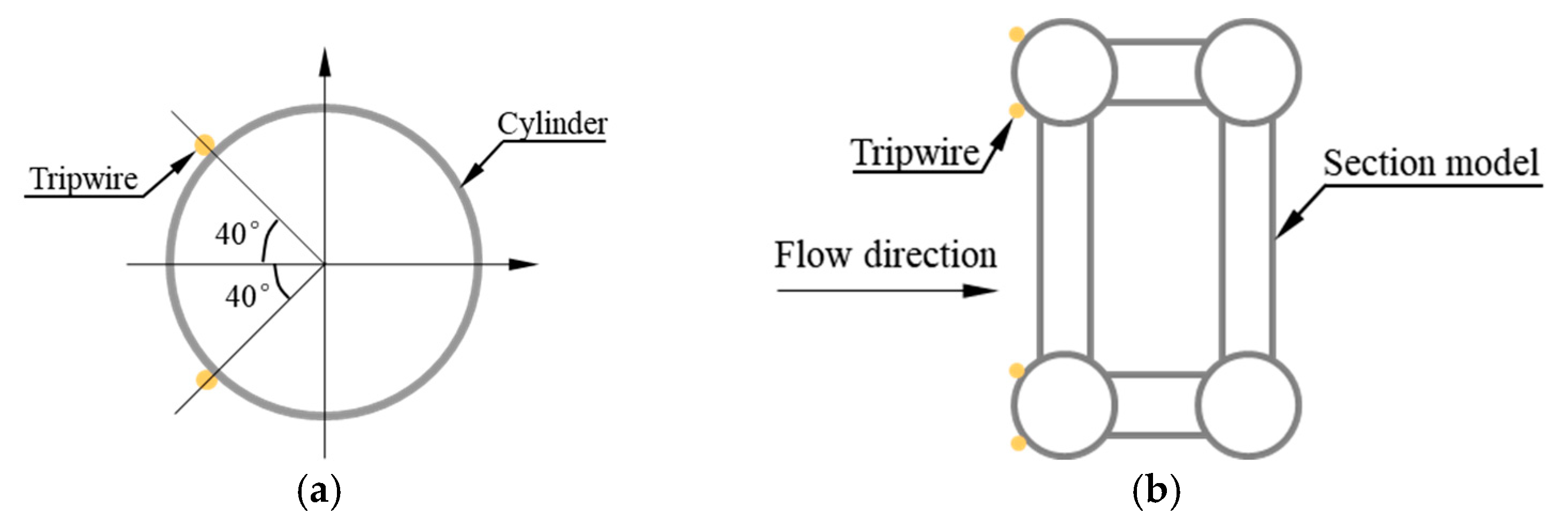
2.1. Design of Section Models

To determine the section types for the arch rib models, a statistical analysis was performed on CFST arch bridges, both completed and under construction, with spans exceeding 150 m [11,12,13]. Among these CFST bridges, approximately 83% featured trussed sections, including three-tube trussed, four-tube trussed, horizontal dumbbell trussed, six-tube trussed, and eight-tube trussed sections. Notably, approximately 81% of CFST truss arches adopted either the four-tube trussed section (Figure 1a) or the horizontal dumbbell trussed section (Figure 1b). Therefore, these two most commonly used section types are selected for the arch rib models in the wind tunnel tests.
In cantilever construction, arch rib segments are assembled using a cable hoisting system, with concrete pouring yet to commence. Therefore, to investigate the wind-induced behaviors of CFST arch ribs during this stage, the sectional models in this study were designed and tested based on hollow steel tubes. Figure 2 provides a schematic diagram of the adopted trussed sections. In the figure, d1, d2, and d4 represent the diameters of the chord, vertical web, and horizontal bracing, respectively, while d3 and d5 denote the spacing between adjacent vertical webs and horizontal bracing. Previous studies [14] on truss bridges have shown that the width-to-height ratio (B/H) has a significant impact on the aerodynamic characteristics of the section. Taking the drag coefficient (CD) of a rectangular section as an example [15], it has been found that CD varies nonlinearly with changes in B/H. CD reaches its maximum value of 3.0 when B/H = 0.7, while it decreases to 2.0 when B/H = 0.5. Additionally, the ratio of the spacing to the diameter of chords also significantly affects the aerodynamic characteristics of the truss section [15]. Therefore, B/H was identified as the key parameter in the wind tunnel test.
To determine the dimensions of arch rib section models for the wind tunnel tests, the detailed dimensions of the four-tube trussed and horizontal dumbbell trussed sections used in CFST arch bridges in practical engineering are summarized in Appendix A. Based on the statistical results, the variation range of B/H is from 0.45 to 0.70. Therefore, the B/H values studied in this test are set as 0.45, 0.58, and 0.70. Based on the commonly used values of d1/H, d2/d1, d2/d4, d3/H, d5/d3, and t/d1 from the statistical results, the values selected for the arch rib section models in this paper are as follows: 0.2, 0.5, 1.0, 1.0, 1.0, and 0.7. Based on Appendix A, the actual sectional heights of four-tube trussed and horizontal dumbbell trussed ribs range from 3.0 to 5.0 m. Considering engineering practice and wind tunnel limitations, a scale ratio of about 1:20 to 1:30 was adopted, and the model height (H) was set to 150 mm. Table 1 lists the specific dimensions of six arch rib section models, where l denotes the length of the section models. The nomenclatures used to identify the specimens are given as follows: FTT and HDT refer to the four-tube trussed section and horizontal dumbbell trussed section, respectively, while I, II, and III denote the specimens with the width-to-height ratios of 0.45, 0.58, and 0.70, respectively.

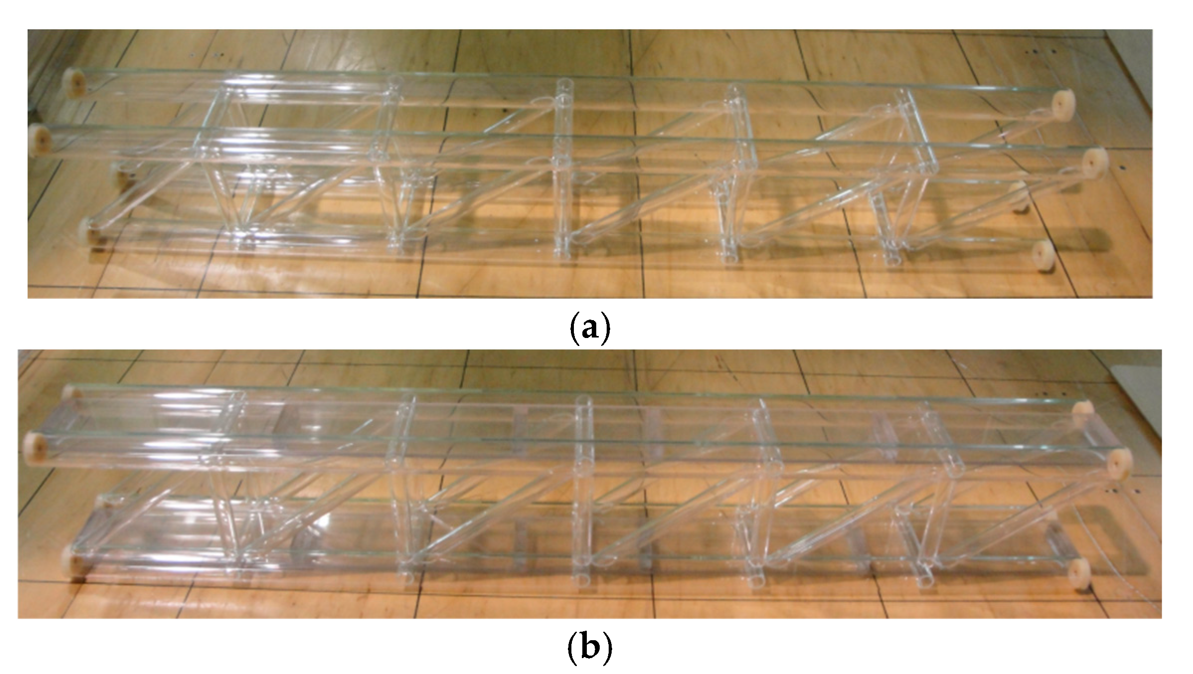
2.2. Manufacturing of Section Models

The arch rib section model was fabricated from acrylic resin and assembled using chords, cross-links, and webs of different lengths. After assembly, the section models of FTT and HDM are shown in Figure 3, with the model HDT-III being the heaviest, weighing 2.167 kg. In addition, to address the issue of the low stiffness of the section models, which caused a longer time for the three-component force to stabilize during tests, six piano wires with a diameter of 0.2 mm were placed on the top, bottom and leeward sides of the section model to enhance its stiffness, as shown in Figure 4. The test wind speeds of 6 m/s and 8 m/s were selected based on Froude scaling principles, corresponding to prototype wind speeds of approximately 25–45 m/s under typical engineering conditions. The drag coefficients (CD) of the model FTT-I, with and without the piano wires, at wind speeds of 8 m/s and 15 m/s under different wind attack angles are shown in Figure 5. From the figure, it is evident that the addition of piano wires has a minimal effect on the aerodynamic force coefficients and can be ignored.
Based on the test design wind speeds of 6 m/s and 8 m/s, as well as the dimensions of the arch rib section models, the calculated Reynolds number (Re) falls within the critical range for wind tunnel tests, which spans approximately from 300 to 300,000. Previous studies [14] have shown that when Re is in the critical range, the boundary layer separation on the cylindrical surface transitions from laminar to turbulent flow and then reattaches to the cylinder, forming separation bubbles that ultimately lead to turbulent separation. During this process, the drag coefficient (CD) of the cylinder varies significantly. Therefore, as shown in Figure 6, the results are heavily influenced by Re, and measures should be taken to increase Re in order to minimize its impact. To achieve this, based on the study by Alam et al. [16], four tripwires were added to the section model, as shown in Figure 7. These tripwires, with a diameter of 1.5 mm, were positioned on the upper and lower chords on the windward side, with an angle of 40° to the horizontal direction. After the addition of the tripwires, CD values at different wind attack angles were measured, as shown in Figure 6. The results indicated that the addition of the tripwires significantly reduced the variation in CD with wind speed, and at a 0° wind attack angle, the CD values became nearly identical. This demonstrates that the method of adding tripwires effectively mitigates the impact of Re.

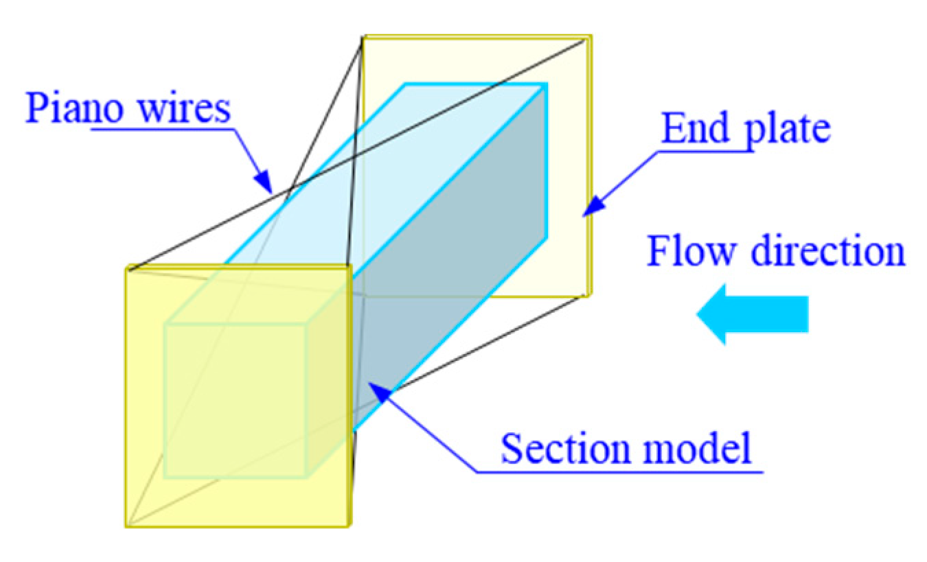
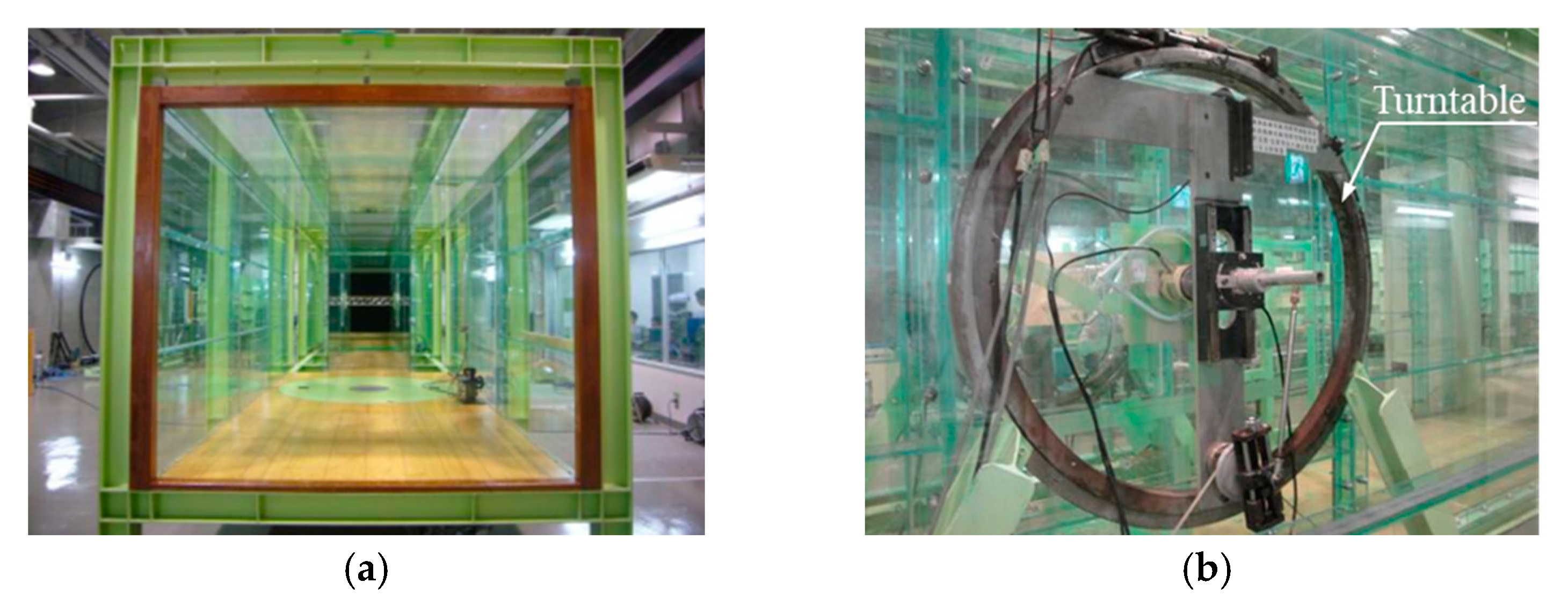
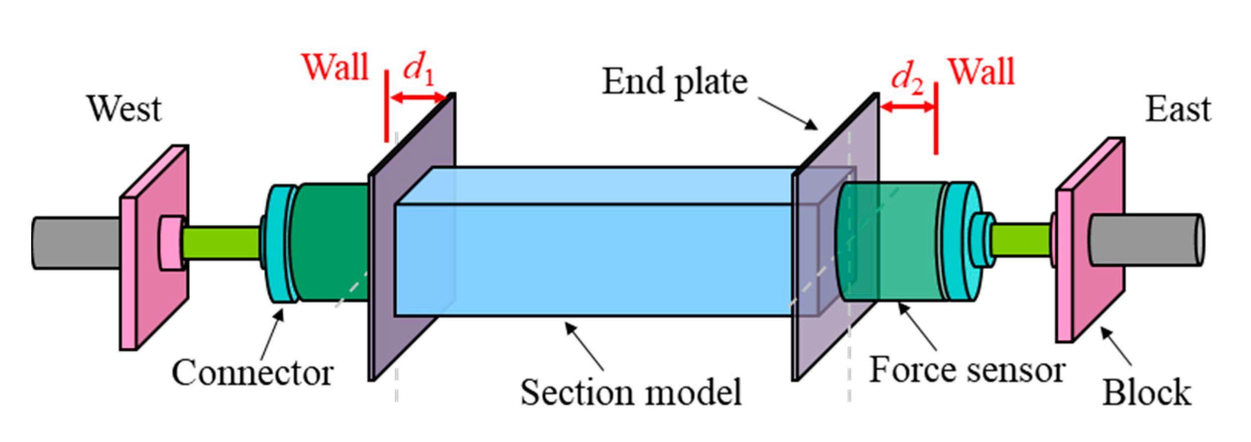
2.3. Test Setup and Measurement

The test was conducted in a direct-current wind tunnel at Kyoto University, Japan, as shown in Figure 8a. The wind tunnel section has a height of 1.8 m and a width of 1 m, with an adjustable wind speed range of 0.2~30 m/s. When the flow field is uniform, the turbulence intensity (Iu) is less than 0.5%. The wind attack angle of the section models was adjusted using a turntable (Figure 8b). During the test, wind speeds of 6 m/s and 8 m/s were used, and the wind attack angle varied from −10° to +10°. The turbulent wind field was generated by a grid made up of rectangular-section columns with a diameter of 40 mm, spaced 200 mm apart both horizontally and vertically.
The drag, lift, and lift moment at both ends of the section model were measured using the LMC-3501 load cell (Nissho Electric Works, Tokyo, Japan), as shown in Figure 9a. The load cell has measurement ranges of 50 N for drag, 50 N for lift, and 5 N∙m for lift moment. The signal was amplified using an MCD-A signal amplifier (A&D HOLON Holdings Co., Ltd., Tokyo, Japan) and converted from analog to digital by the DF-3Z32-2 A/D converter (A&D HOLON Holdings Co., Ltd., Tokyo, Japan). A pitot tube was used to calibrate the wind speed in the uniform flow, a grid was employed to generate turbulence, and X-type hot wires (Golden Mountain Enterprise Co., Ltd., Gaoxiong, China) were used to measure the instantaneous wind speed in the turbulent flow (Figure 9b). To ensure the validity of the measured result, several steps were taken: before the tests, the Pitot tube (Golden Mountain Enterprise Co., Ltd., Gaoxiong, China) was calibrated against a reference velocity source to ensure accurate pressure-to-velocity conversion; during testing, repeated runs under identical conditions were performed to assess the repeatability of the measurements.

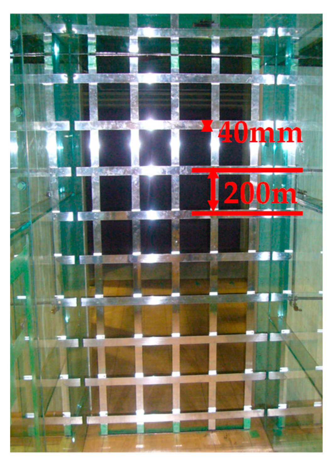
2.4. Generation of Turbulent Wind Field

A turbulence-generating grid was employed in the experiment to create a turbulent wind field. The grid consisted of rectangular-section columns with a cross-sectional diameter of 40 mm, arranged in both horizontal and vertical directions at 200 mm intervals (as shown in Figure 10). After the grid was installed, a hot-wire anemometer was used to calibrate the mean wind speed under turbulent conditions. The fan rotational speed was incrementally increased to 150 rpm, 250 rpm, 350 rpm, 450 rpm, and 550 rpm, with hot-wire measurements taken at each stage. The anemometer sampled data at a frequency of 1 kHz for a duration of 30 s. Using the calibration data, the corresponding inflow wind speed for each set of measurements was determined, allowing the relationship between fan speed and mean wind speed in turbulent flow to be established. This relationship was subsequently used to adjust the fan speed in order to achieve the target test wind speed during the experiment.

2.5. Measurement Process

The procedure for measuring the force coefficients of the FTT and HDT section models involves several key steps: installation and calibration of force sensors, wind speed calibration, model installation, and data collection. During the model installation, the assembled section model was connected to the end plates, which were then attached to the force sensors using connectors. The distance between the end plates and the wind tunnel side walls was ensured to be equal on both sides (d1 = d2, as shown in Figure 11). A spirit level was used to confirm that the top surface of the section model was horizontally aligned along both the axial and vertical directions. During data collection, different wind attack angles (−10° to +10°) and various wind conditions, including no wind, 6 m/s, 8 m/s, and post-wind stoppage, were considered. The data acquisition frequency was set at 1 kHz, with a collection duration of 65 s. Measurements were taken only after the force sensor readings had stabilized. The force coefficients of the section model were then calculated based on the calibration factors of the force sensors.

3. Experimental Results

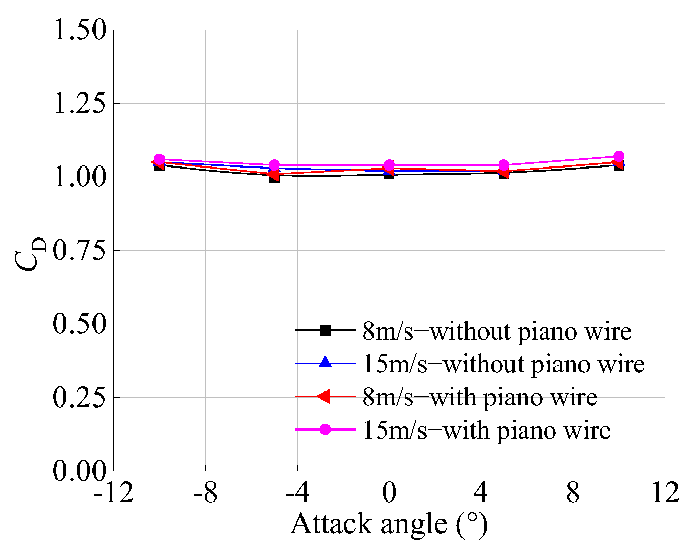
3.1. Aerodynamic Force Coefficient

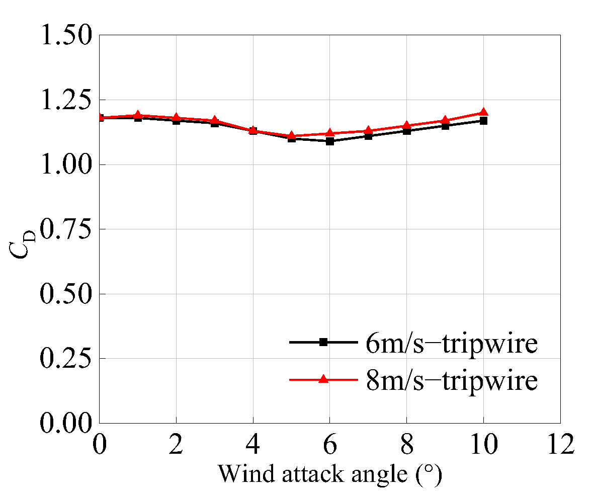
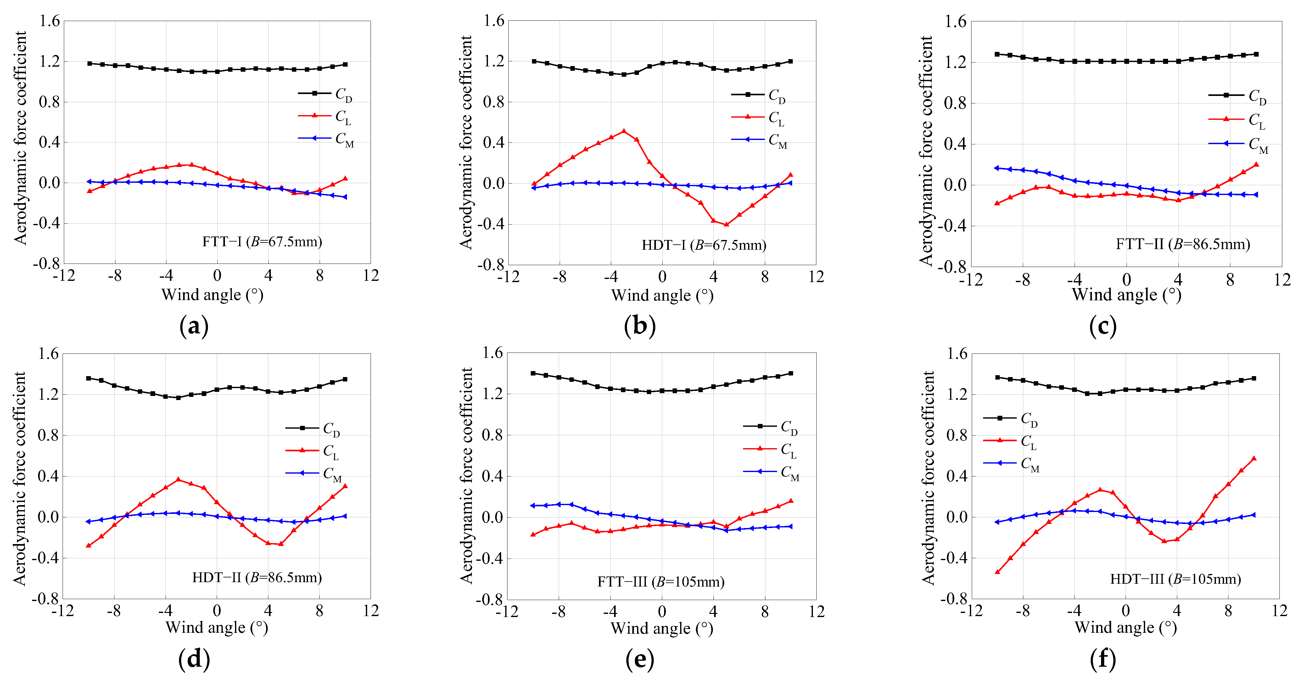
3.1.1. Aerodynamic Force Coefficients Under Laminar Flow

Figure 12 presents the aerodynamic force coefficients of six section models under laminar flow, with wind attack angles ranging from −10° to +10°. The coefficients obtained from the wind tunnel tests include the drag coefficient (CD), lift coefficient (CL), and lift moment coefficient (CM). As shown in the figure, the aerodynamic forces are primarily dominated by drag, followed by lift, with lift moment values being relatively small. In addition, both CD and CM show minimal variations with changes in wind attack angle across all models, while CL exhibits different variations depending on the section model. For the FTT sections, CL shows only a slight variation with wind attack angle. In contrast, for HDT the sections, CL varies more noticeably: at smaller absolute wind attack angles (e.g., −3° to +5° for HDT-I), CL decreases as the angle increases, whereas at larger absolute wind attack angles (e.g., −10° to −3° and +5° to +10° for HDT-I), CL exhibits the opposite behavior. CL of HDT-I exhibited a counterintuitive reduction when the wind angle increased from −3° to +5°, which may be attributed to flow interference between upper and lower chords or unsteady wake behavior. Furthermore, the figure shows that near a wind attack angle of 0°, the slopes of the curves for FTT-I and all HDT section models are negative, indicating that these sections are unstable and may potentially experience galloping.
The variation in aerodynamic force coefficients with model width under laminar flow at a 0° wind attack angle is presented in aerodynamic force coefficient Figure 13. As shown, with varying model widths, both FTT and HDT models exhibit only slight changes in CD, which remains around 1.2, and in CM, which stays close to 0. The lift coefficient (CL) for HDT models is slightly higher than for FTT models, with average values calculated as 0.1 for HDT models and 0 for FTT models.

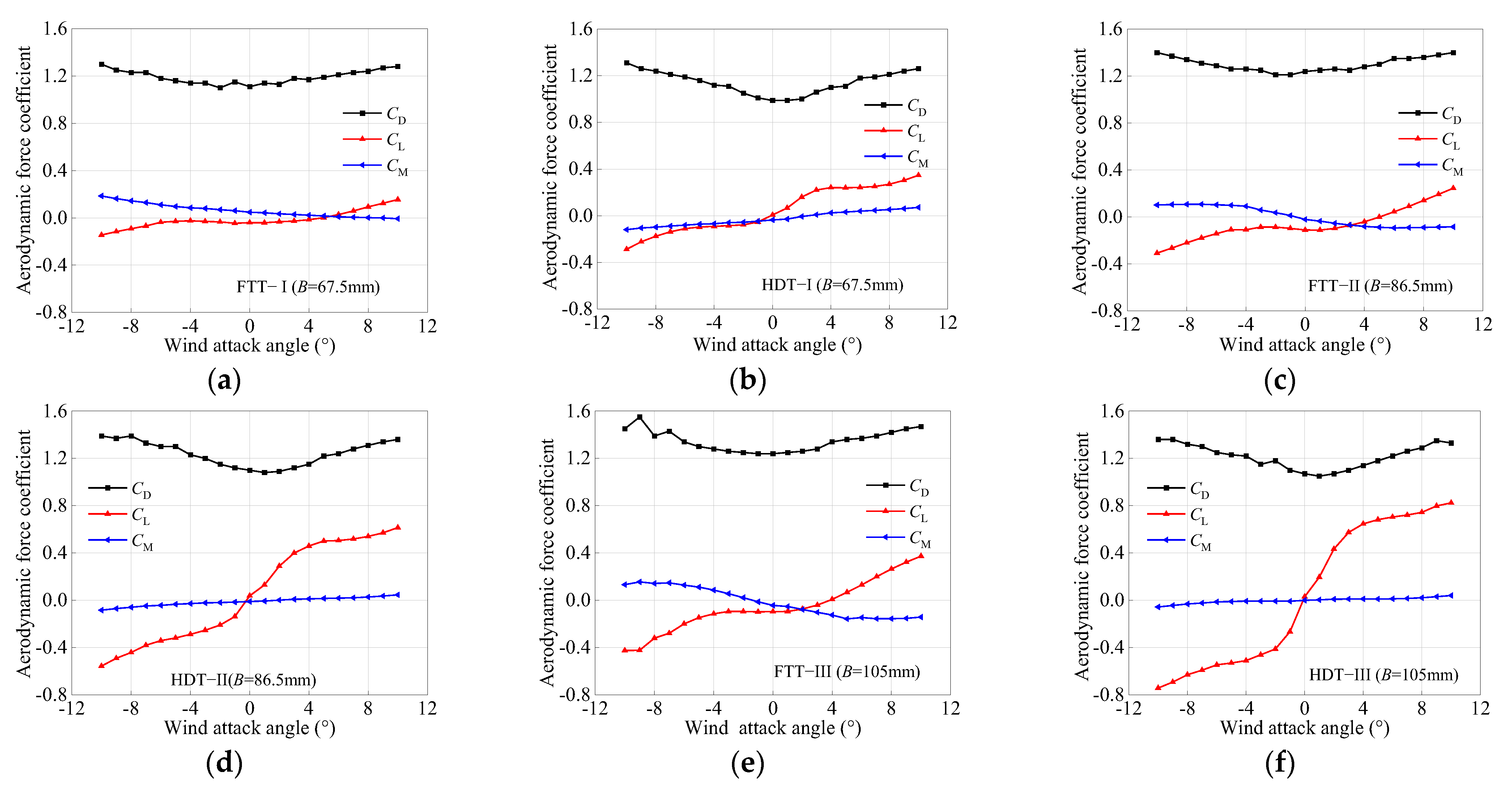
3.1.2. Aerodynamic Force Coefficients Under Turbulent Flow

The aerodynamic force coefficients of six section models in the turbulent wind field, with wind attack angles ranging from −10° to +10°, are shown in Figure 14. The aerodynamic forces are primarily dominated by drag, with minimal variation in CD as the wind attack angle changes. At a 0° wind attack angle, CD is at its minimum and slightly increases with the absolute value of the wind attack angle. CL increases with the wind attack angle, with the increase becoming more significant as the model width increases. Noticeable fluctuations in CM were observed under turbulent flow, suggesting possible variations in aerodynamic center or asymmetric vortex shedding. Additionally, CM remains small and exhibits little variation with wind attack angle.
The aerodynamic force coefficients of all section models at a 0° attack wind angle in the turbulent wind field are listed in Table 2. It can be observed that minimal changes with varying model widths are shown for both FTT and HDT section models, while CL and CM remain relatively small, close to zero.

3.2. Aerodynamic Admittance Function

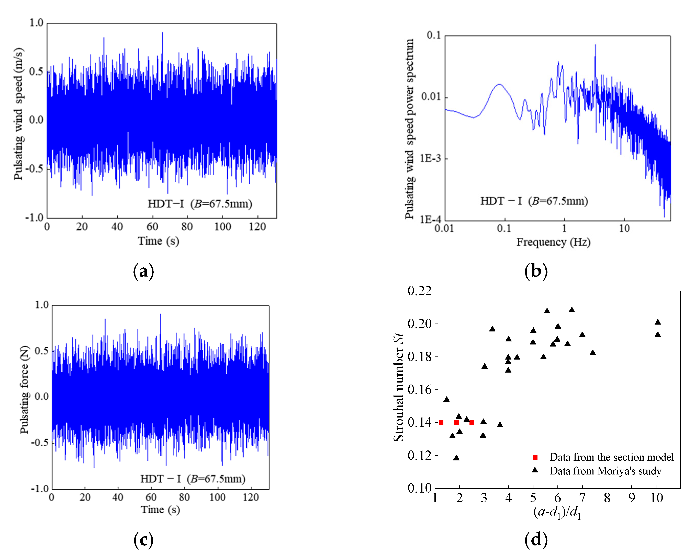
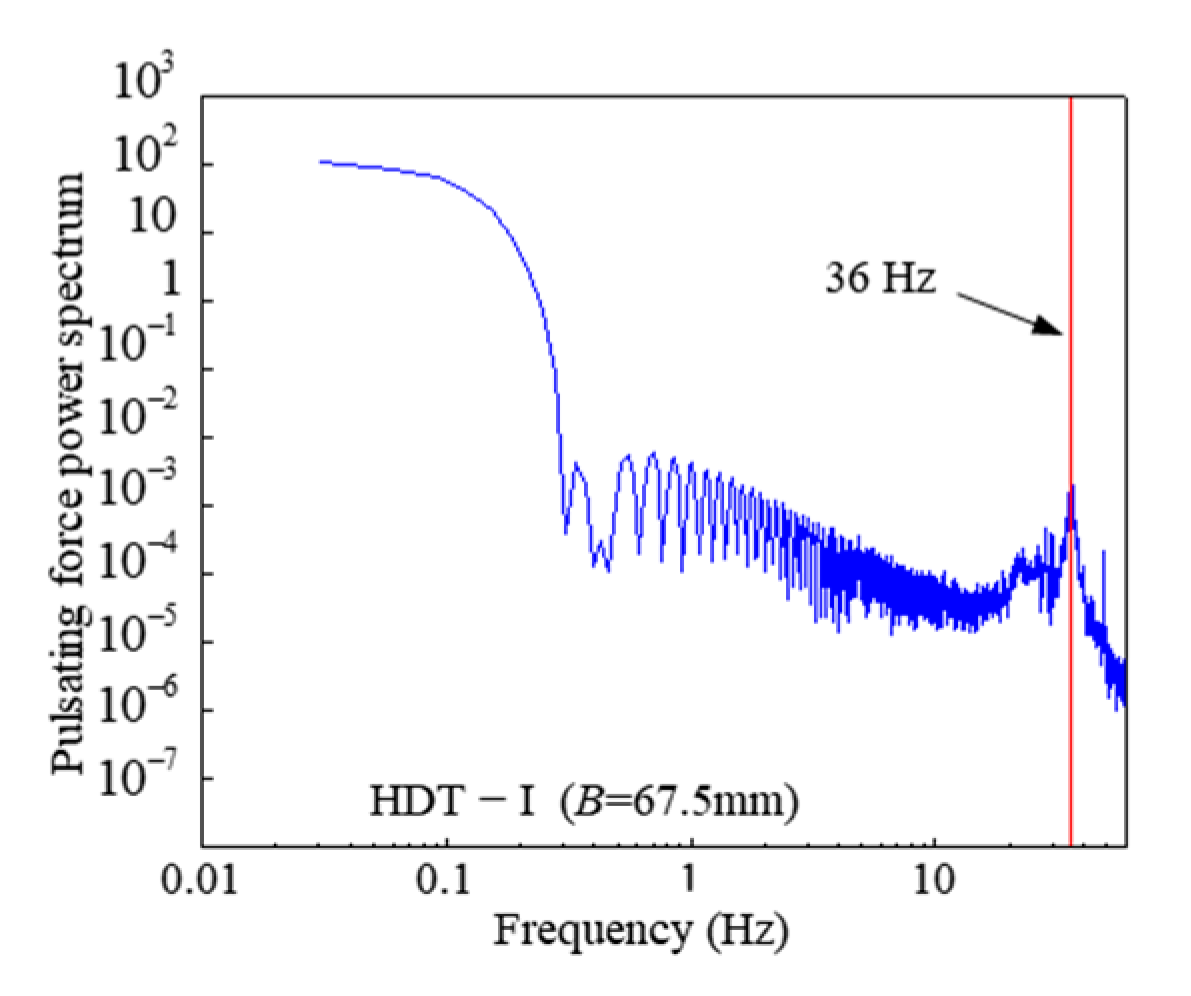
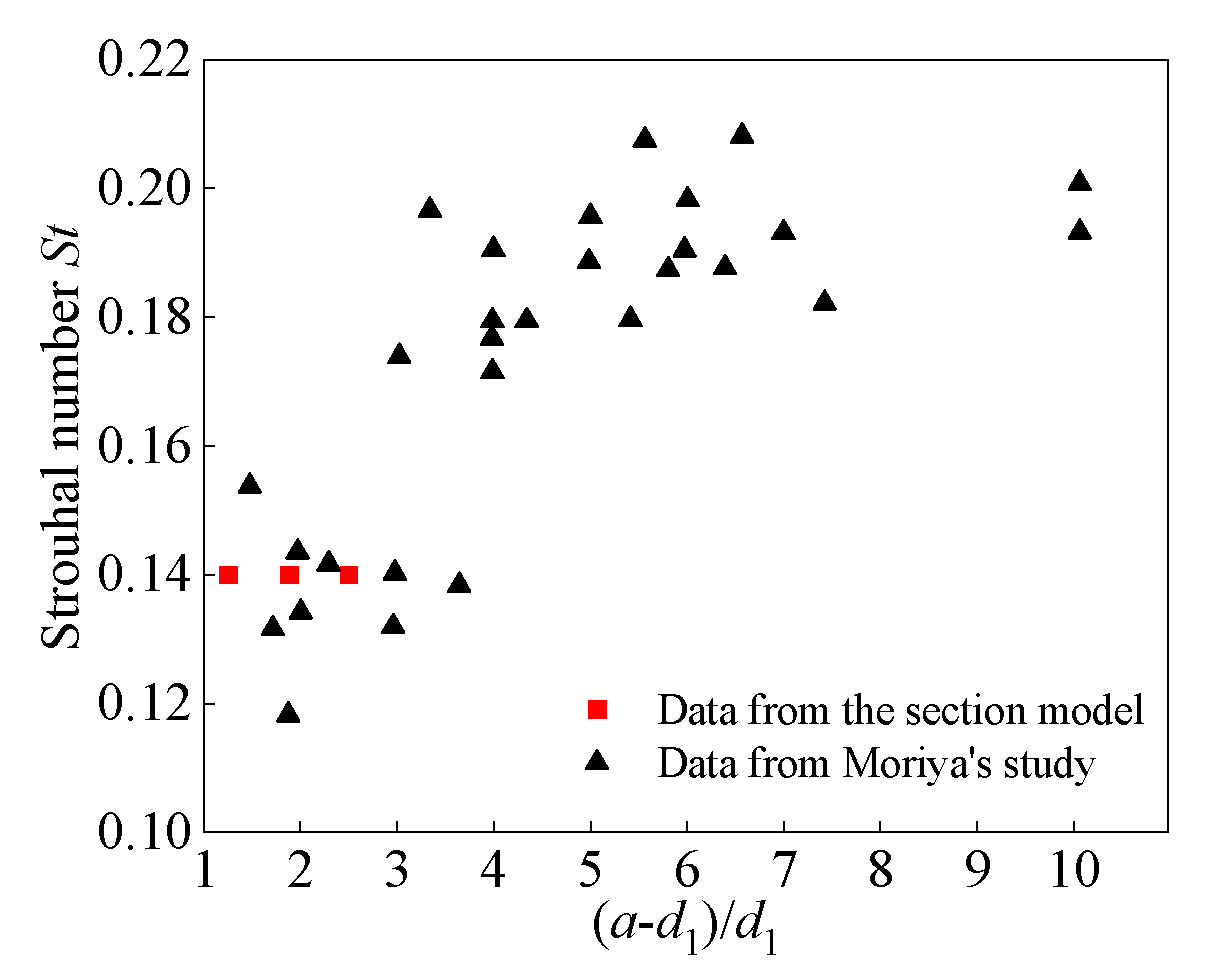
3.2.1. Power Spectrum Estimation
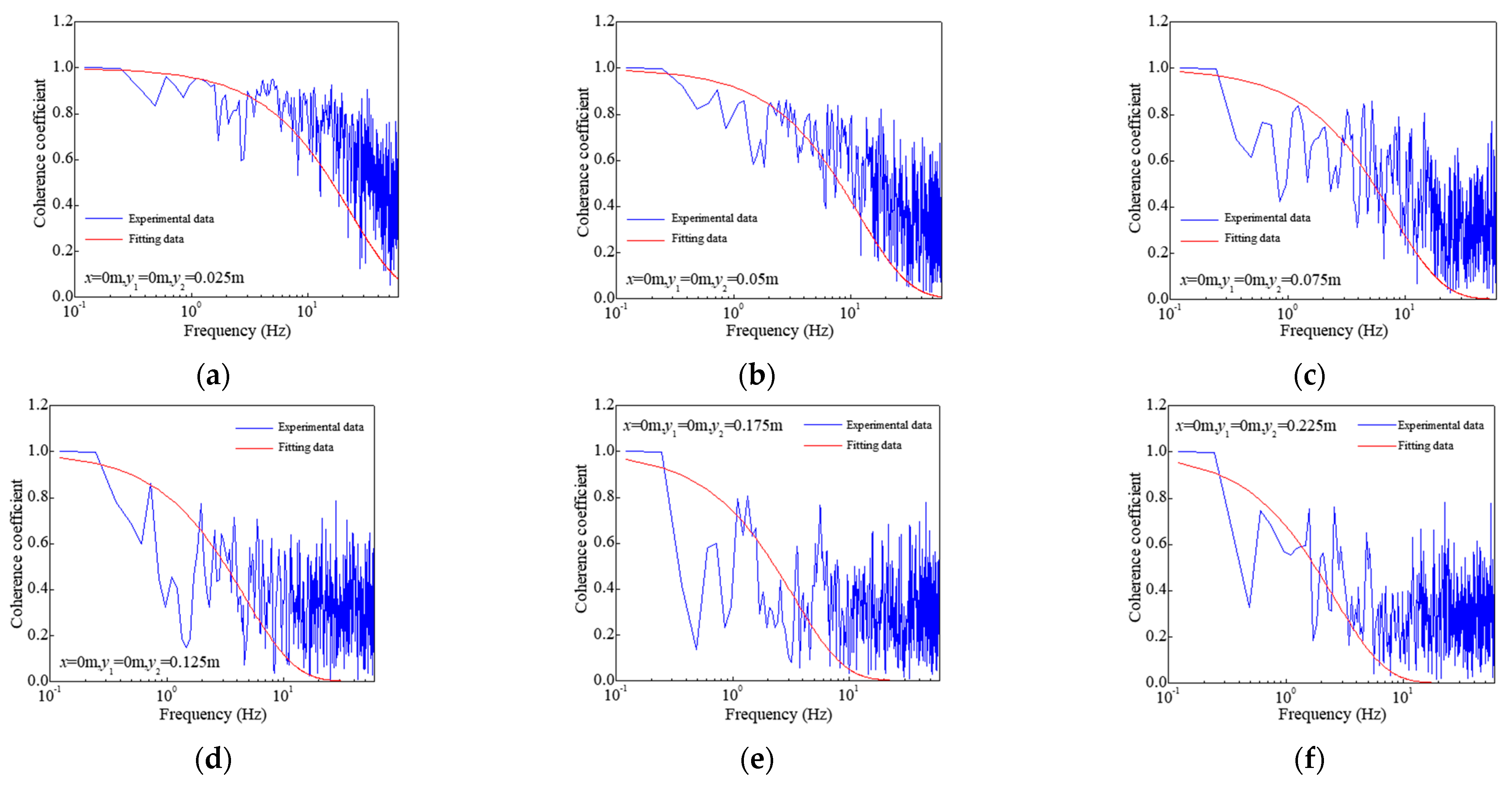
To obtain the aerodynamic admittance function (AAF), it is necessary to convert the time series data into power spectral density. In this study, the Welch method is used to estimate the power spectrum. The specific procedure of the Welch method is shown as follows: First, divide the signal x(n) into segments, ensuring a 50% overlap between adjacent segments. Next, apply a non-rectangular window to each segment, perform an N-point Fourier transform, and then square the modulus of the result, divided by N. Finally, average the power spectra of all segments to obtain the power spectral estimate of x(n). Meanwhile, a low-pass filter is used to filter out frequencies above 60 Hz, thereby eliminating noise interference from the measurement system. As an example, the data measured from the HDT-I model are used. Figure 15a and Figure 15b present the fluctuating wind speed time series and its power spectral density, respectively, while Figure 15c and Figure 15d exhibit the fluctuating drag time series and its power spectral density.
Notably, it can be found from Figure 15d that a distinct peak in the fluctuating wind power spectrum for the HDT-I model appears around a frequency of 40 Hz. To determine if this peak is caused by vortex shedding, an analysis of the drag time series under laminar flow for this model is conducted. Figure 16 shows the drag power spectrum obtained from the drag time series of the HDT-I model under laminar flow. The frequency corresponding to the peak in Figure 16 is 36 Hz. By applying this frequency to the Strouhal number formula St = nd1/U, the value of St is calculated to be 0.14. According to the study by Moriya et al. [17], the relationships between St and the spacing ratio (ad1)/d1 for two cylinders in line are shown in Figure 17, where the red points represent the calculations of the section model in this study. By comparing the data in Figure 17, it is evident that the frequency corresponding to the peak in Figure 17 is indeed the vortex shedding frequency of the section model. Therefore, this effect of vortex shedding should be eliminated in the subsequent calculations of the aerodynamic admittance coefficient.

3.2.2. Decay Factor

The fluctuating wind speeds at different points in the wind tunnel were measured to calculate the cross-power spectrum S D ˜ y 1 , y 2 , n and auto-power spectra S D ˜ y 1 , n and S D ˜ y 2 , n of the wind speed. By substituting these results into Equation (1), the coherence coefficient S D ˜ y 1 , y 2 , n can be obtained. The coherence coefficient curve calculated from the experimental data at x = 0 m is shown in Figure 16. In addition, the coherence coefficient can also be fitted using a formula, exp λ n y 1 y 2 / U , that is related to the decay factor λ. The calculated results match the experimental data best when λ = 14, as shown in Figure 18.
c o h D ˜ y 1 , y 2 , n = S D ˜ y 1 , y 2 , n / S D ˜ y 1 , n S D ˜ y 2 , n

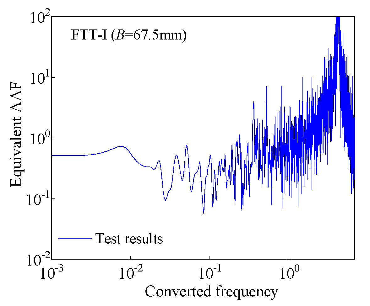
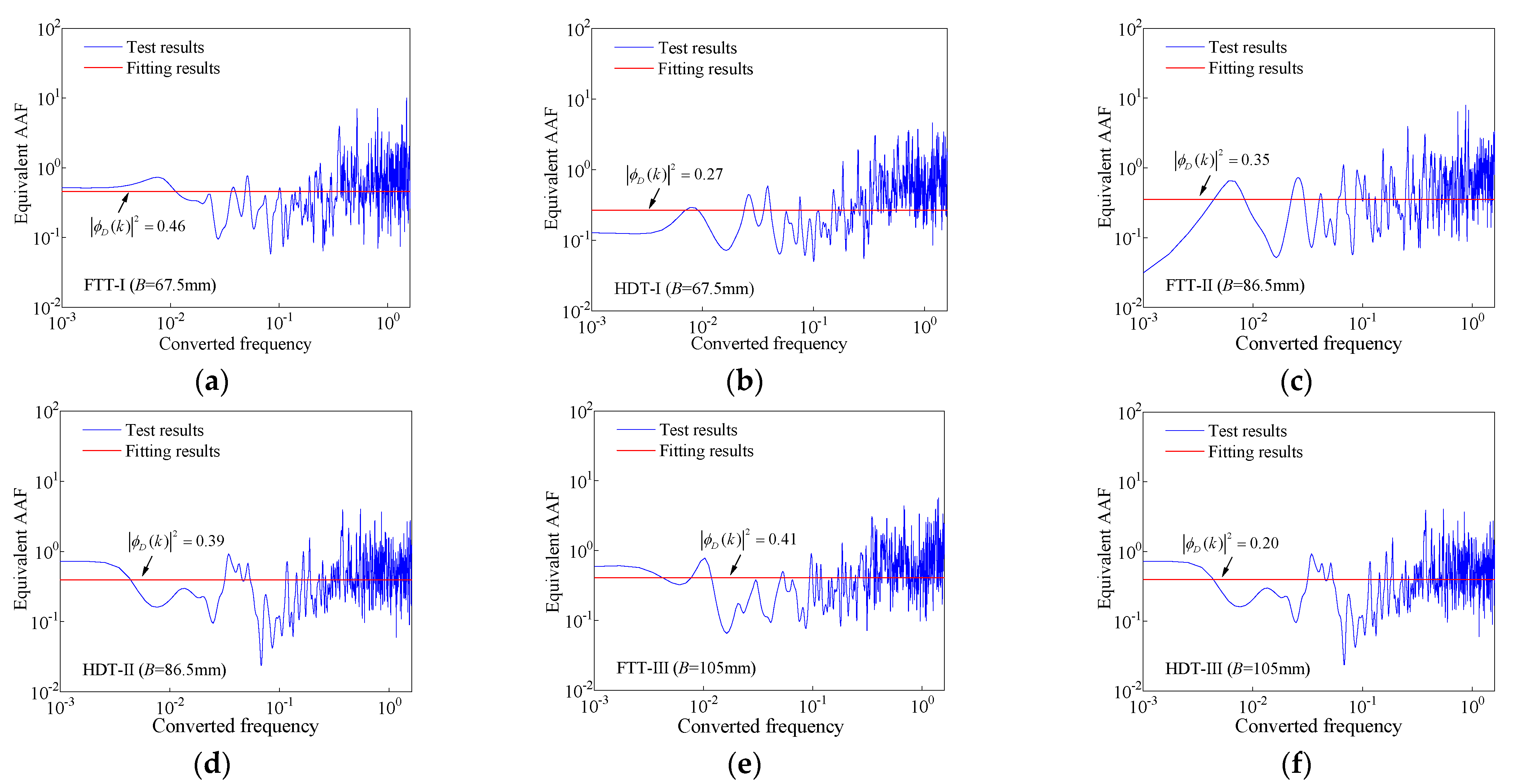
3.2.3. Equivalent Aerodynamic Admittance Function

The equivalent AAF ϕ D k 2 for all section models can be obtained by substituting the calculated aerodynamic power spectrum S D ˜ a l l n , fluctuating wind power spectrum S u n , and decay factor λ into Equation (2). In this equation, n is the frequency; k represents the converted frequency, and k = nB/U; U is the incoming wind velocity; ρ denotes the air density; and B, H, and L0 are the width, height, and length of the section model, respectively.
ϕ D k 2 = 1 ρ U C D H L 0 2 S D ˜ a l l n S u n L 0 + U λ n exp λ n L 0 U U λ n
Figure 19 presents the test results of the equivalent AAF for the section model FTT-I. As shown in the figure, the equivalent AAF exhibits a peak in the high-frequency region, followed by a sharp decrease as the converted frequency increases. According to the power spectrum analysis in Section 3.2.1, this peak is induced by vortex shedding. Considering the significance of the equivalent AAF in the low-frequency range, the fitting process is primarily focused on the low-frequency region to eliminate the influence of vortex shedding on the test results, and the comparison between the test and fitted results of the equivalent AAF is shown in Figure 20.
As observed, the mean values of the equivalent AAFs for both the four-tube trussed and horizontal dumbbell trussed models remain nearly constant across different frequencies, allowing for a linear approximation in fitting. The fitted equivalent AAF values for models FTT-I, II, and III are 0.46, 0.35, and 0.41, respectively, while those for HDT-I, II, and III are 0.27, 0.39, and 0.20, respectively. It can be found that the fitted equivalent AAFs of the section models varied from 0.20 to 0.46, reflecting the influence of different structural parameters. Given the relatively small variations in equivalent AAFs among different models, the maximum value of 0.46 can be adopted as an approximate reference.

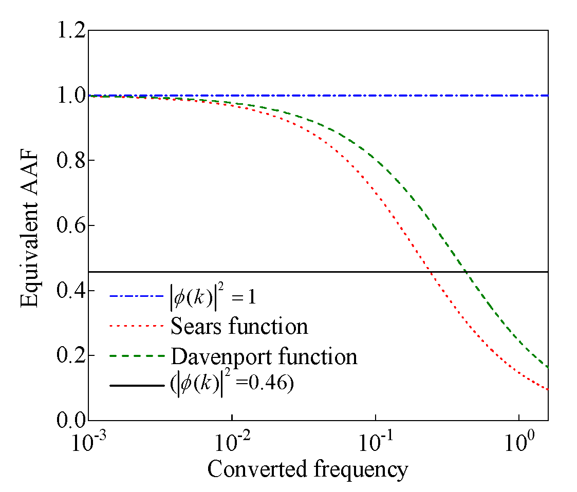
3.2.4. Comparisons of the Measured Equivalent AAFs with Other Commonly Used AAFs

In existing buffeting analyses of CFST arch bridges, due to the lack of measured equivalent AAF data for the arch ribs, empirical formulas (such as the Sears function and Davenport function) are commonly used for approximation, or it is assumed that the sectional aerodynamic forces are equal to the corresponding quasi-steady aerodynamic forces (i.e., the equivalent AAF is taken as 1.0).
The simplified Sears function, originally derived by Sears for airfoils and later simplified by Liepmann, and the Davenport function, proposed by Davenport for bridges, are expressed in Equations (3) and (4), respectively. In these equations, k denotes the converted frequency, and k = nB/U.
ϕ k 2 = 1 1 + π k
ϕ k 2 = 1 c k 2 c k 1 + e c k
Figure 21 compares the measured equivalent AAFs with other commonly used AAFs. As shown, the Sears and Davenport functions decrease as the converted frequency increases. At lower converted frequencies, these functions yield values higher than the measured equivalent AAFs, while at higher frequencies, their values fall below the measured results. Furthermore, the experimentally obtained equivalent AAF (0.46) is considerably lower than 1.0, demonstrating that the assumption of sectional aerodynamic forces being equal to quasi-steady aerodynamic forces is not reasonable.

4. Buffeting Response

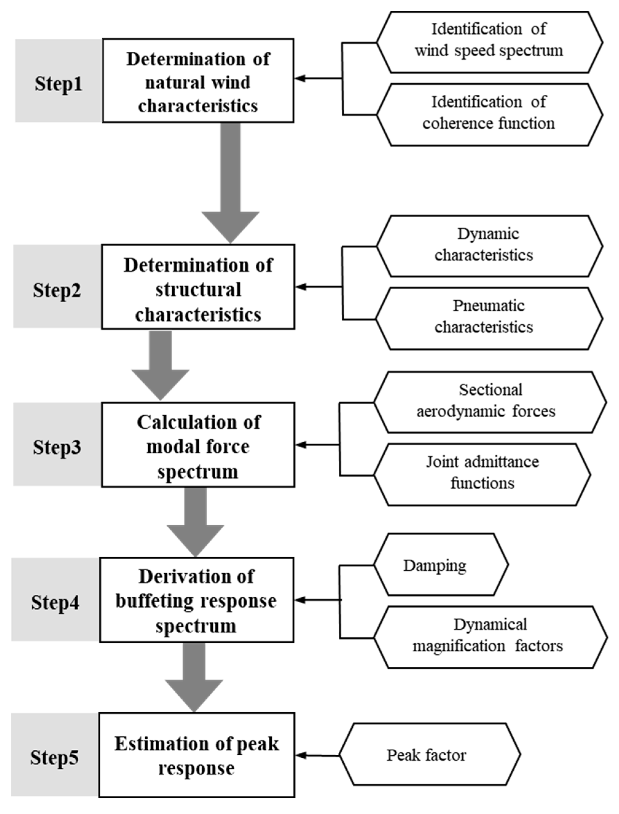
4.1. Buffeting Analysis Program

Due to the lack of measured wind field data and structural aerodynamic parameters, previous studies on the buffeting response of CFST arch bridges have primarily depended on empirical formulas or simplified analytical methods, which may result in considerable deviations from actual conditions. To improve accuracy, this study utilizes the experimentally obtained three-component force coefficients and equivalent AAFs from Section 3 to analyze the buffeting response of cantilevered arch ribs, incorporating the influence of the curved arch axis.
Given that the spans of existing CFST arch bridges do not exceed 600 m, the maximum horizontal projection length of cantilevered arch ribs during construction is limited to 300 m. Moreover, due to the relatively sparse spectral distribution of cantilevered arch structures, the coupling effects between modes can be disregarded, enabling the buffeting response to be determined through modal superposition. Consequently, a frequency-domain analysis approach was adopted to assess the buffeting response of cantilevered arch ribs.
The frequency-domain buffeting analysis is based on the following assumptions: (1) the fluctuating wind induced by turbulence can be considered a stationary random process; (2) the quasi-steady assumption is adopted; (3) the coupling effects between structural modes are neglected, and structural vibrations are considered as the superposition of individual modal responses; (4) the turbulence-induced fluctuations are assumed to be much smaller than the mean wind speed, allowing the fluctuating wind load to be expressed as a linear function of the fluctuating wind velocity; (5) the most unfavorable wind direction is assumed to be perpendicular to the bridge axis. Additionally, the strip assumption is commonly used in buffeting analysis, converting the three-dimensional flow field into a two-dimensional plane flow field. This simplification assumes that the bridge is sufficiently long and straight, enabling wind loads at any given section to be representative of those at other sections.
Figure 22 illustrates the procedure for buffeting analysis, which consists of five main steps as follows:
(1)
Determination of natural wind characteristics, including the identification of the wind speed spectrum and coherence function;
(2)
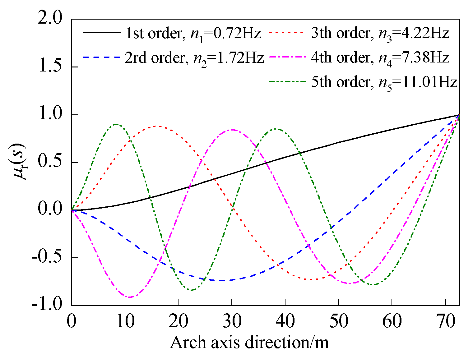
Determination of structural characteristics, involving the evaluation of sectional aerodynamic force coefficients, AAFs, structural frequencies, and mode shapes;
(3)
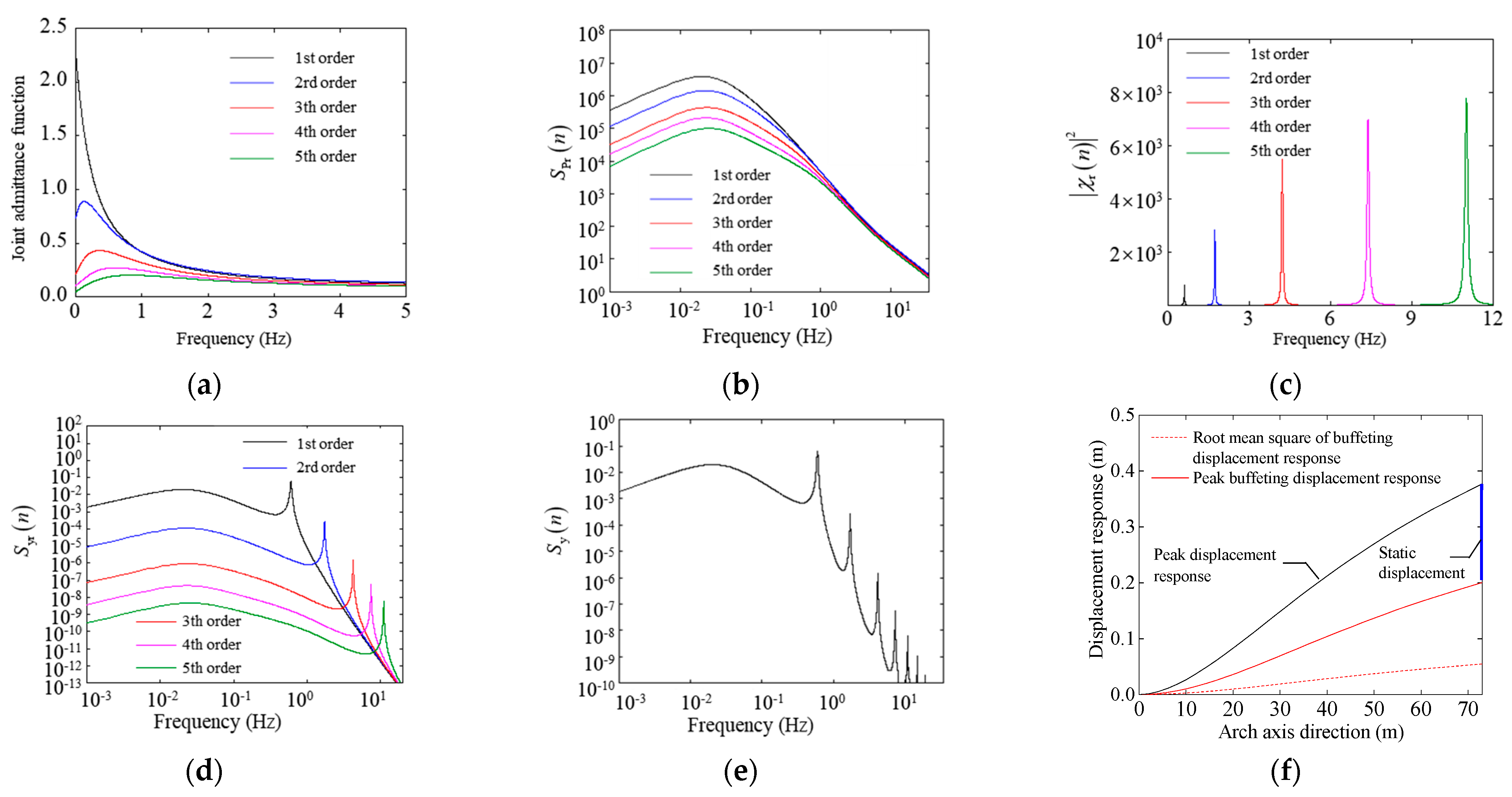
Calculation of modal force spectrum, including the determination of sectional aerodynamic forces and joint admittance functions;
(4)
Derivation of buffeting response spectrum, involving the assessment of structural damping and dynamic amplification factors;
(5)
Estimation of peak response, which can be determined using the peak factor method.
In addition, the proposed buffeting analysis program follows the following assumptions: (1) the pulsating wind caused by turbulent flow can be considered as a smooth random process; (2) quasi-constant assumptions; (3) the coupling effect between structural modes is neglected and the structural vibration is assumed to be expressed as a superposition of different modal responses; (4) the turbulent pulsation is assumed to be much smaller than the mean wind speed, so the pulsating wind load can be expressed as a linear function of the pulsating wind speed; (5) the most unfavorable wind speed direction is assumed to be is assumed to be perpendicular to the direction of the bridge axis. Meanwhile, the strip assumption is employed to transform the three-dimensional flow field into a two-dimensional plane flow field; i.e., the cantilever CFST arch ribs are assumed as long enough and flat, and then the wind load can be expressed by the wind load at any section.

4.2. Verification of the Buffeting Analysis Procedure

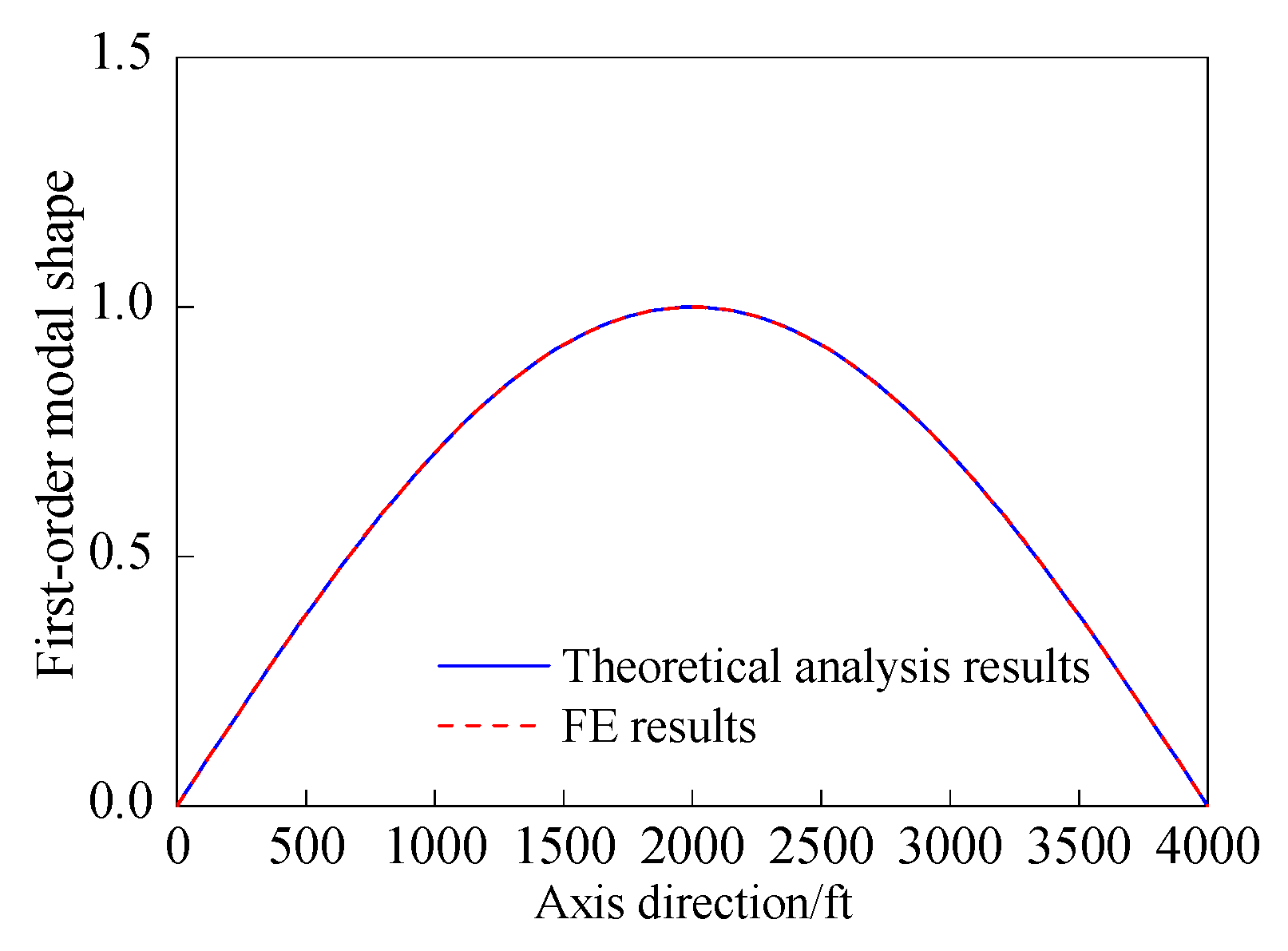
4.2.1. Buffeting Analysis of Suspension Cables

To validate the accuracy of the buffeting analysis procedure, a buffeting analysis example of the suspension cable from Davenport’s paper [18] was selected for comparison. In this example, the suspension span is 4000 ft (1219.2 m), with a sag of 270 ft (82.3 m) and a height of 200 ft (61.0 m) above the ground. The wind pressure acting on the upper cable per unit length is given by 3.3 × 10⁻⁵U2, where U is the design average wind speed, taken as 100 ft/s (30.5 m/s). The surface friction coefficient is 0.01, and the wind speed spectrum follows the Davenport spectrum. The first-order modal period in the horizontal direction of the suspension is 15 s, with a mode shape of sin (πx/l), while the second-order modal period is 8 s, with a mode shape of sin (2πx/l).
The finite element (FE) model of the suspension cable was established using ABAQUS to analyze the mode shapes. The obtained mode shapes were then compared with the theoretical analysis results from Davenport’s paper [18], as shown in Figure 23. The good agreement between the FE and theoretical results confirms that the FE model can accurately capture the structural mode shapes. Furthermore, the buffeting displacements of the suspension cable, as calculated by the buffeting analysis procedure, were 3.93 m for the first-order mode and 0.97 m for the second-order mode, with a maximum deviation of only 0.8% from the theoretical results.

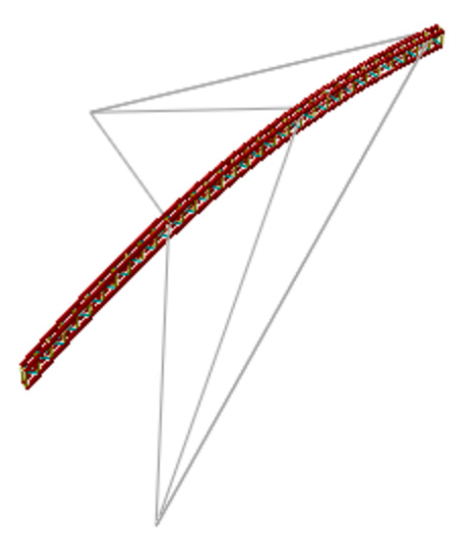
4.2.2. Buffeting Analysis of Cantilevered Arch Rib

To further validate the accuracy of the buffeting analysis procedure, the buffeting response of the Shenzhen Rainbow Bridge during cantilever construction was analyzed (Figure 24). This bridge is a through-type CFST tied arch bridge, with a main span of 150 m and a rise-to-span ratio of 1/4.5. The main arch ribs feature a four-tube trussed section, with dimensions of 3 m in height and 2 m in width. The chord members consist of four steel tubes with dimensions of ϕ750 mm × 12 mm [19]. The construction method involves cable hoisting, with the arch ribs prefabricated in seven segments at the factory and then transported to the site for assembly. During the cantilever assembly phase, the arch ribs were subjected to a grade 12 typhoon, causing the maximum displacement at the cantilever end to reach 0.41 m [20,21]. Subsequently, a modal analysis was performed to obtain the first 5 order frequencies and vibration patterns (Figure 25).
Using the joint admittance function formula (Equation (5)), the relationship between the joint admittance function and frequency for the first five modes is shown in Figure 26a. The modal force spectrum, obtained from Equation (6), is plotted against frequency in Figure 26b. By computing the unit mass and wind resistance of the cantilevered arch, the logarithmic decrement in the aerodynamic damping ratio is determined using Equation (7). Substituting this value into the dynamic amplification factor formula (Equation (8)) provides the relationship between the dynamic amplification factor and frequency for different modes, as shown in Figure 26c. Further, applying the dynamic amplification factor in Equation (9) yields the modal displacement spectrum as a function of frequency, illustrated in Figure 26d. Finally, summing the modal displacement spectra according to Equation (10) results in the structural displacement spectrum, as presented in Figure 26e.
J r n 2 = 1 N r 2 0 s 0 s K 2 s 1 K 2 s 2 c o h s 1 , s 2 , n μ r s 1 μ r s 2 d s 1 d s 2
S P r n = S P 0 n J r n 2
δ r = 1 n r 0 s P s ¯ U s ¯ μ 2 s d s 0 s m s μ 2 s d s
χ r n 2 = 1 n / n r 2 2 + δ r / π 2 n / n r 2 1
S y s , n = χ r n 2 m ω r 2 2 S P r n
S y s , n = S y r n μ r 2 s
In the above equations, n represents frequency, s1 and s2 are any two points on the arch rib; J r n 2 denotes the joint admittance function; c o h s 1 , s 2 , n denotes the coherence function; μ r s is the mode shape of the r-th order; Nr is a coefficient, calculated as 0 s μ r s μ r s d s ; K(s) is the wind speed height correction factor at point s; S P r n represents the modal force spectrum of the r-th order; δ r is the logarithmic decrement in the aerodynamic damping ratio corresponding to the r-th mode; U ¯ s is the mean wind speed at point s; P ¯ s represents the drag force acting on the cantilevered arch at point s under uniform flow; us is the fluctuating wind speed at point s; χ r n 2 denotes the dynamic amplification factor; nr is the frequency corresponding to the r-th mode; S y r n is the displacement spectrum of the r-th mode; m is the unit mass along the arch axis; ωr is the angular frequency of the r-th mode; S y s , n is the displacement spectrum at point s on the arch axis.
Figure 26f illustrates the computed buffeting displacement, static displacement, and peak displacement of the cantilevered arch of Shenzhen Rainbow Bridge under wind load. The results show that the peak displacement at the cantilever end reaches 0.37 m. Field measurements indicate that the maximum displacement under wind load was 0.41 m, with a deviation of 9.8%. This confirms that the proposed buffeting analysis procedure can effectively capture the wind-induced response of the cantilevered arch rib.

4.3. Influence of Analysis Parameters on Wind-Induced Response in Buffeting Analysis

In the buffeting analysis of CFST arch bridges, the lack of field-measured wind field data and structural aerodynamic parameters often leads to the use of empirical formulas or simplified methods. For instance, when the equivalent AAF is unavailable, the Sears empirical formula is typically used. Similarly, to simplify buffeting response calculations, the coherence function is often assumed to be independent of frequency, and the joint admittance function is treated as a frequency-independent function. Therefore, it is essential to assess the applicability and accuracy of these approximations in buffeting analysis.

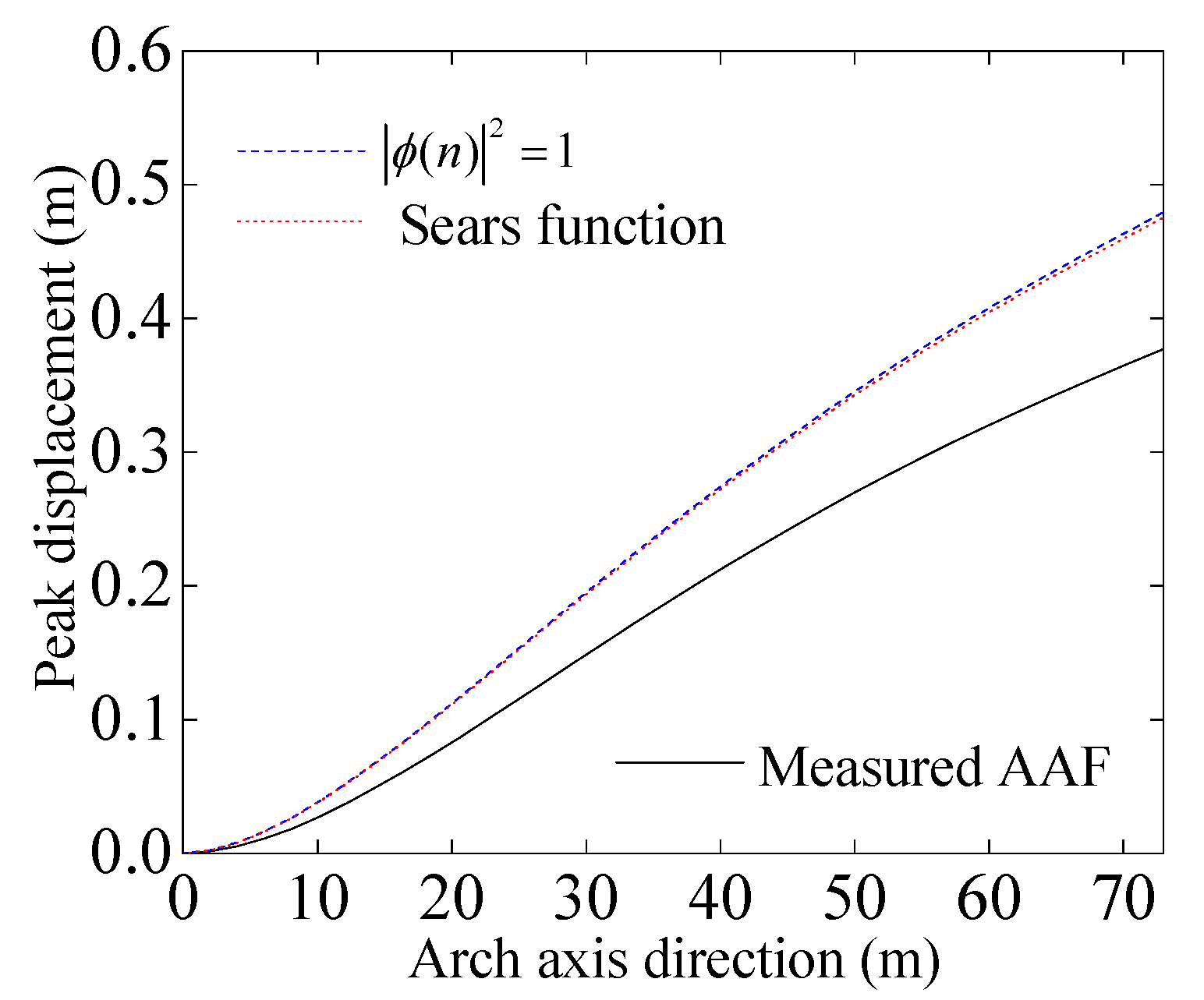
4.3.1. Influence of Equivalent AAF

As discussed in Section 3.2.4, the equivalent AAF in the buffeting analysis of CFST arch bridges is often approximated as a constant value of 1.0 ( ϕ n 2 = 1 ) or calculated using the Sears function. To evaluate the accuracy of these assumptions, a comparative analysis was conducted considering three cases: assuming a constant AAF of 1.0, adopting the Sears function, and using measured AAF data. Figure 27 presents a comparison of peak responses obtained under these different approaches. The results indicate that the peak displacements calculated using ϕ n 2 = 1 and the Sears function are 27.1% and 26.1% higher, respectively, than that derived from measured data. This suggests that using either ϕ n 2 = 1 or the Sears function provides a more conservative estimation of peak displacement.

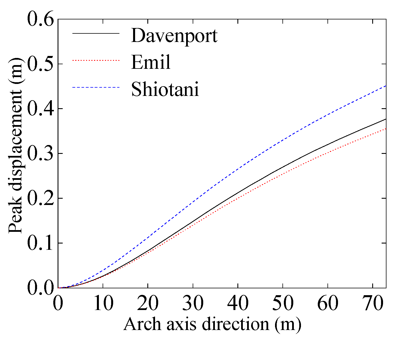
4.3.2. Influence of Coherence Function

Many researchers have investigated coherence functions based on field measurements, revealing their exponential distribution characteristics. Davenport [22] formulated a coherence function that accounts for frequency, spatial separation, and mean wind speed, as presented in Equation (11), with the decay coefficient c set to 7. Emil [14] later refined this model, suggesting c = 10 based on further analysis. Meanwhile, Shiotani [23] proposed a more simplified expression dependent solely on spatial distance, as shown in Equation (12), where Ls is assigned a value of 50.
c o h s 1 , s 2 , n = exp c n Δ s U ¯ = exp c n s 1 s 2 U ¯
c o h s 1 , s 2 , n = exp Δ s L s = exp s 1 s 2 L s
Notable differences exist among the coherence functions proposed by various researchers, along with significant discrepancies in the recommended decay coefficients for the same function. Therefore, different coherence functions proposed by Davenport, Emil, and Shiotani are incorporated into the buffeting analysis program to evaluate their influence on buffeting response results. Figure 28 compares the peak responses derived from different coherence functions. The results show that the peak responses obtained using Davenport’s and Emil’s coherence functions are similar, with Emil’s being 5.7% lower than Davenport’s. In contrast, the peak response calculated with Shiotani’s function is 20.0% higher than that of Davenport. Given that Shiotani’s function is independent of frequency, it serves as a more conservative approximation.

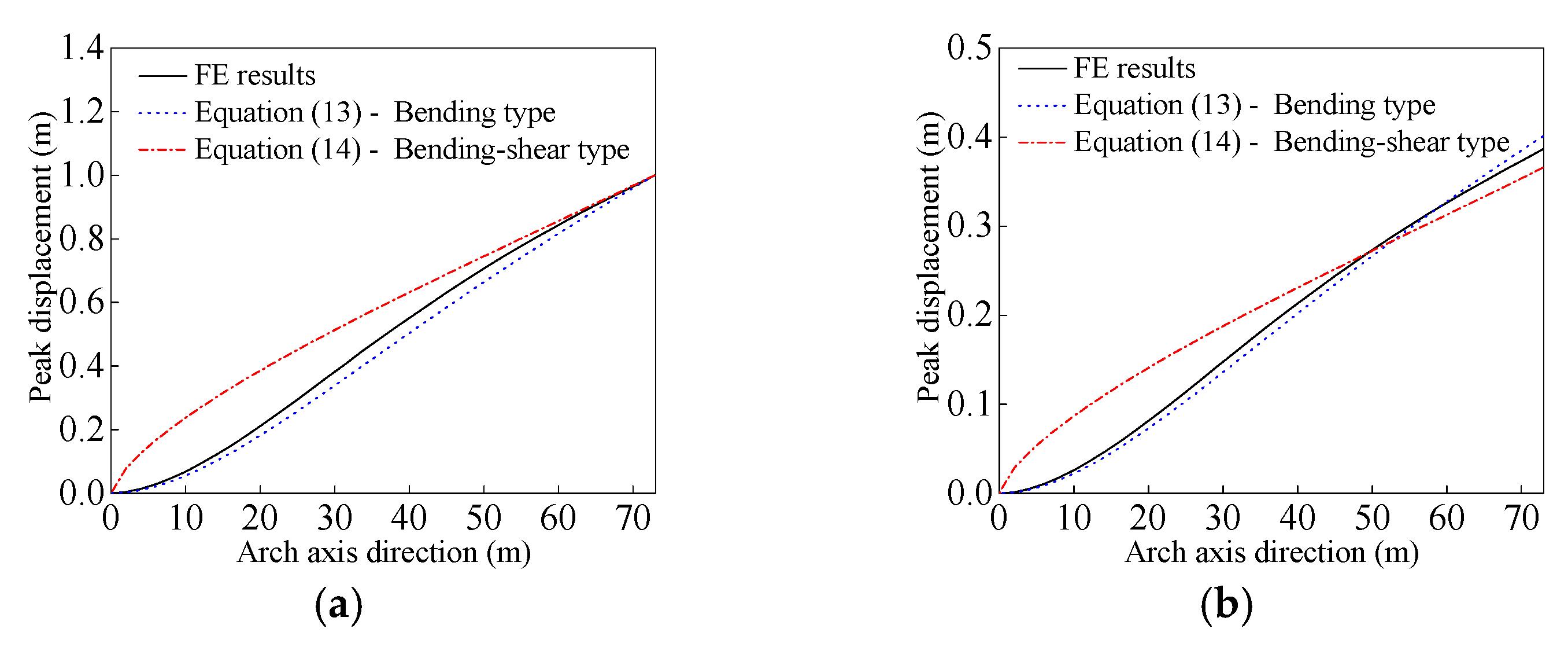
4.3.3. Influence of Shape Function

The Chinese load code for the design of building structures (GB 50009-2012) [24] provides simplified calculation formulas for the first-order modal shapes of high structures. These formulas are categorized into bending-type and bending-shear-type approximations, as shown in Equations (13) and (14). Equation (13) is applicable to high structures modeled based on bending-type behavior, where H is the total height of the structure and y represents the coordinate along the height, with the ground level defined as the zero point. Equation (14) is used for high-rise buildings modeled based on bending-shear-type behavior, where shear wall behavior is dominant.
u 1 y = 6 y 2 H 2 4 y 3 H + y 4 3 H 4
u 1 y = tan π 4 y H 0.7
Taking the Shenzhen Rainbow Bridge as an example, Figure 29a compares the first-order mode shapes obtained from ABAQUS analysis with those calculated using the approximate formulas in Equations (13) and (14). The results indicate that the bending-type formula provides a mode shape that closely aligns with the ABAQUS analysis, whereas the bending-shear-type formula shows significant deviation. In addition, Figure 29b compares the peak responses obtained using different modal shapes. It is observed that the peak response obtained using the ABAQUS-derived modal shape closely aligns with that from the bending-type formula, with a maximum displacement difference of only 1.2%. Conversely, the peak response derived from the shear-type approximation formula exhibits notable discrepancies in both magnitude and distribution compared to the other results. These findings suggest that the bending-type approximation formula in Equation (13) can be reliably used to represent the first-order modal shape of cantilevered CFST arch ribs.

4.3.4. Influence of the Number of Modes

It is stated in Chinese code GB 50009-2012 [24] that for wind-induced vibration analysis of tall cantilevered structures, such as chimneys and towers, the spectral distribution is generally sparse, with the first-order mode playing a dominant role. As a result, only the first-order mode is typically considered. Frequency analysis of the cantilevered arch of the Shenzhen Rainbow Bridge in Figure 25 also shows a sparse spectral distribution. To evaluate the feasibility of determining the buffeting response of the cantilevered arch ribs based solely on the first-order mode, the contributions of different modes to the buffeting response were analyzed.
Figure 30 compares the buffeting and peak responses obtained by considering the first 10 modes versus only the first mode. The results show minimal differences, with the buffeting response differing by only 0.3% and the peak response by just 2.6%. These findings confirm the dominant influence of the first-order mode, suggesting that considering only the first-order mode is sufficient for buffeting analysis of cantilevered CFST arch ribs.

5. Conclusions

In this paper, the wind tunnel tests of arch rib section model with four-tube trussed and horizontal dumbbell trussed sections were conducted, the aerodynamic force coefficients and equivalent aerodynamic admittance functions (AAFs) of all section models were obtained, and the wind-induced responses of the cantilevered CFST arch rib during the construction phase were analyzed. The main conclusions are drawn as follows:
(1)
The aerodynamic forces acting on the section models of cantilevered CFST arch ribs are primarily governed by drag, with aerodynamic force coefficients showing minimal variation with changes in model width. Under laminar flow conditions, the aerodynamic force coefficients for the four-tube trussed section are 1.2 for drag, 0 for lift, and 0 for lift moment, while those for the horizontal dumbbell trussed section are 1.2, 0.1, and 0, respectively.
(2)
By measuring the fluctuating wind speeds at various points in the wind tunnel and fitting the decay factor, the equivalent AAFs for the arch rib section were determined. The equivalent AAFs for both four-tube trussed and horizontal dumbbell trussed sections can be approximated by a horizontal line and conservatively taken as 0.46.
(3)
Based on the measured aerodynamic force coefficients and equivalent AAFs, a buffeting analysis program for the cantilevered arch rib was developed and validated through comparisons of the classical theoretical analysis results and field measurements.
(4)
The influence of various parameters on the peak response in the buffeting calculation of cantilevered CFST arch ribs was analyzed, including the equivalent AAFs, coherence function, first-order mode shape, and the number of structural modes.
In this study, laminar flow was used for simplicity to measure basic aerodynamic characteristics of the cantilevered CFST arch ribs. However, since real atmospheric wind is usually turbulent and varies with height, future tests will consider turbulent boundary layer flow to improve the accuracy and realism of the aerodynamic analysis. In addition, CFD simulations on specific CFST bridge structures will be conducted to further validate the buffeting analysis program and gain deeper insights into the aerodynamic behavior of these structures under varying wind conditions.

Author Contributions

Q.H.: Investigation, Methodology, Software, Formal Analysis, Writing, Writing—Review and Editing. X.W.: Investigation, Software, Formal Analysis, Writing—Review and Editing. S.Z.: Methodology, Formal Analysis, Writing—Review and Editing. D.L.: Writing—Review and Editing. All authors have read and agreed to the published version of the manuscript.

Funding

The research work in this paper was supported by the National Natural Science Foundation of China (Grant No. 52308164) and the National Postdoctoral Support Program of China (Grant No. GZB20230963).

Data Availability Statement

The original contributions presented in the study are included in the article, further inquiries can be directed to the corresponding author.

Conflicts of Interest

Author Xinrong Wu was employed by the company Journal of Building Structures Editorial Office, Beijing, China. The remaining authors declare that the research was conducted in the absence of any commercial or financial relationships that could be construed as a potential conflict of interest.

Appendix A. Statistical Data on the Sectional Dimensions of CFST Truss Arch Bridges Constructed in China

Table A1. Cross-sectional dimensions for four-tube trussed sections (unit: m).
CFST ArchesBHB/Hd1d2d3d4d5
Beijing–Hangzhou Grand Canal Bridge2.003.700.5410.850.402.500.73-
Sanmenkou Crossing Sea Bridge2.405.300.4530.800.404.000.402.00
Shitanxi Bridge1.603.000.5330.550.222.700.401.35
Jialingjiang Bridge2.003.500.5710.760.353.500.35-
Caihong Bridge2.003.000.6670.750.252.000.402.00
Yongjiang Bridge2.004.300.4650.820.38-0.38-
Changqing Bridge1.803.400.5290.700.25-0.30-
Shenxigou Bridge2.304.050.5680.850.34-0.34-
Songao Bridge2.604.800.5420.800.40-0.60-
Jiangwan Bridge2.20--0.700.35-0.40-
Lingfeng Bridge1.832.400.7630.700.351.670.351.67
Shawan Bridge1.603.000.5330.61----
Daduhe Bridge1.703.300.5150.70----
Taiping Lake Bridge3.007.280.4121.280.618.000.81-
Maocaojie Bridge3.204.000.8001.000.554.000.654.00
Rongzhou Bridge-4.00-1.020.464.00--
Yangtze River Bridge4.147.000.5911.220.616.000.716.00
Meixihe Bridge4.405.000.8800.920.355.000.355.00
Nanlidu Bridge2.104.000.5250.920.344.000.344.00
Jingyang River Bridge-5.00-1.020.435.000.435.00
Yellow River Grand Canal Bridge6.507.500.8671.50----
Note: ‘-’ denotes unavailable data; the definitions of sectional parameters in the table are provided in Section 2.1 and Figure 2.
Table A2. Cross-sectional dimensions for horizontal dumbbell trussed sections (unit: m).
CFST ArchesBHB/Hd1d2d3T
Nanpu Bridge2.555.200.4900.850.61--
Shuidao Grand Canal Bridge2.505.500.4551.000.605.000.70
Yongjiang Grand Canal Bridge---1.02-5.00-
Qiandao Lake 1# Bridge2.505.000.5001.000.405.00-
Jiantiao Bridge1.904.400.4320.800.405.90-
Changfeng Bridge2.404.500.5331.000.505.000.80
Beipanjiang Bridge2.505.400.4631.000.455.500.80
Shengmi Bridge3.005.000.6000.900.303.00-
Longtanhe Bridge2.40--0.900.404.000.50
Sanshan West Bridge-3.50-0.700.35--
Wangcun Grand Canal Bridge2.003.80.5260.750.303.25 0.50
Wujiang Bridge---0.60-5.07-
Panjiahe Bridge1.402.700.5190.600.43--
Heishipu Bridge2.504.000.6251.000.436.00-
Lijiang Bridge1.753.500.5000.710.33--
Junzhou Bridge1.803.000.6000.750.302.60-
Yuanyangjiang Bridge1.803.300.5450.750.25--
Fuxing Bridge2.604.500.5780.950.404.000.60
Pubugou Bridge2.002.800.7140.760.302.000.65
Qijiadu Yellow River Bridge1.703.500.4860.700.332.500.40
Wushan New Longmen Bridge2.404.500.5331.000.503.000.80
Caoejiang Bridge2.254.000.5630.900.40-0.50
Tongde Bridge2.053.500.5860.750.35--
Nanhuan Bridge1.803.500.5140.750.403.000.52
Rainbow Bridge2.405.500.4361.000.225.000.78
Zhongshan Bridge1.753.400.5150.750.302.250.65
Yesanhe Railway Bridge2.203.800.5790.800.423.250.52
Shengzhou Caoejiang Bridge2.003.000.6670.750.353.50-
Yonghe Bridge3.008.000.3751.220.619.20-
Baoding Bridge-3.50-0.750.35--
Qingganhe Bridge2.402.401.0001.000.404.000.50
Note: ‘-’ denotes unavailable data; the definitions of sectional parameters in the table are provided in Section 2.1 and Figure 2.

References

  1. Gu, M.; Su, L.K.; Quan, Y.; Huang, J.; Fu, G. Experimental study on wind-induced vibration and aerodynamic mitigation measures of a building over 800 meters. J. Build. Eng. 2022, 46, 103681. [Google Scholar] [CrossRef]
  2. Wang, J.Y.; Wang, F.; Chen, X.M.; Wei, J.; Ma, J. Investigation of wind load characteristics of cantilevered scaffolding of a high-rise building based on field measurement. Energy Build. 2025, 328, 115123. [Google Scholar] [CrossRef]
  3. Zhou, S.H.; Liao, H.L.; Zheng, S.X.; Li, Y.L. Experimental study on wind resistance performance model of Yajisha Bridge. In Proceedings of the 13th National Bridge Academic Conference, Shanghai, China, 16–19 November 1998; pp. 566–571. (In Chinese). [Google Scholar]
  4. Wang, Z.G.; He, J.; Sun, B.N.; Lou, W.J.; Yu, X.M. Wind tunnel tests and calculation analysis of wind resistance stability segment model of steel-concrete arch bridge. In Proceedings of the 8th National Conference on Structural Engineering, Yunnan, China, 22–26 October 1999; pp. 208–213. (In Chinese). [Google Scholar]
  5. Luo, X.; Pan, Y.Y. Buffeting analysis for concrete-filled tubular arch bridge in time domain. J. Southwest Jiaotong Univ. 2000, 35, 475–479. (In Chinese) [Google Scholar]
  6. Lu, B.; Hu, Z.T. Study of wind resistance of long-span concrete-filled steel tube arch bridge erected by integral lifting method. World Bridges 2005, 3, 68–71. (In Chinese) [Google Scholar]
  7. Yan, Z.T. Study on Wind-Induced Vibration of Long Span Half-Through Arch Bridges. Ph.D. Thesis, Chongqing University, Chongqing, China, 2006. (In Chinese). [Google Scholar]
  8. Claudio, B.; Claudio, M. Aeroelastic Phenomena and Pedestrian-Structure Dynamic Interaction on Non-Conventional Bridges and Footbridges; Firenze University Press: Florence, Italy, 2010. [Google Scholar]
  9. Yu, H.G. Study on Aerodynamic Parameter Identification and Wind-Induced Responses of Long-Span Arch Bridges. Ph.D. Thesis, Tongji University, Shanghai, China, 2008. (In Chinese). [Google Scholar]
  10. JTG/T 3360-01-2018; Wind-Resistant Design Specification for Highway Bridges. Ministry of Transport of the People’s Republic of China: Beijing, China, 2018.
  11. Chen, B.C.; Liu, J.P.; Wei, J.G. Concrete-Filled Steel Tubular Arch Bridges; China Commu, Press Co. Ltd. & Springer: Beijing, China, 2023. [Google Scholar]
  12. Zheng, J.L.; Du, H.L.; Mu, T.M.; Liu, J.P.; Qin, D.Y.; Mei, G.X.; Tu, B. Innovations in design, construction, and management of Pingnan third bridge-the largest-span arch bridge in the world. Struct. Eng. Int. 2021, 32, 134–141. [Google Scholar] [CrossRef]
  13. Zheng, J.L.; Wang, J.J. Concrete-filled steel tube arch bridges in China. Engineering 2018, 4, 143–155. [Google Scholar] [CrossRef]
  14. Simiu, E.; Scanlan, R.H. Wind Effects on Structures: Fundamentals and Applications to Design, 3rd ed.; John Wiley & Sons, Inc.: Hoboken, NJ, USA, 1996; pp. 297–298. [Google Scholar]
  15. Chen, Z.Q. Bridge Wind Engineering; China Communications Press: Beijing, China, 2005. (In Chinese) [Google Scholar]
  16. Alam, M.M.; Zhou, Y.; Zhao, J.M.; Flamand, O.; Boujard, O. Classification of the tripped cylinder wake and bi-stable phenomenon. Int. J. Heat Fluid Flow 2010, 31, 545–560. [Google Scholar] [CrossRef]
  17. Masaru, M.; Hiroshi, S.; Masaru, K.; Mikio, A. Fluctuating force acting on two circular cylinders in series. Proc. Mech. Soc. 1983, 7, 1364–1372. (In Japanese) [Google Scholar]
  18. Davenport, A.G. The response of slender line-like structures to a gusty wind. Proc. Inst. Civ. Eng. 1962, 23, 389–408. [Google Scholar] [CrossRef]
  19. Qian, X.G. Construction and Monitoring Technique Research on Shenzhen Rainbow Bridge. Master’s Thesis, Hunan University, Changsha, China, 2002. (In Chinese). [Google Scholar]
  20. Chen, Z.G. Wind resistant design and practice of Shenzhen Rainbow Bridge. West-China Explor. Eng. 2004, 10, 194–196. (In Chinese) [Google Scholar]
  21. Qian, X.G. Wind resistant design and practice of arch rib construction for Shenzhen North Station Bridg. Highway 2001, 8, 75–78. (In Chinese) [Google Scholar]
  22. Davenport, A.G. The dependence of wind load upon meteorological parameters. In Proceedings of the International Research Seminar on Wind Effects on Buildings and Structures, Ottawa, ON, Canada, 11–15 September 1967; pp. 19–82. [Google Scholar]
  23. Shiotani, M.; Iwatani, Y. Correlations of wind velocities in relation to the gust loadings. In Proceedings of the Third International Conference on Wind Effects on Building and Structures, Tokyo, Japan, 6 September 1971; pp. 57–67. [Google Scholar]
  24. GB 50009-2012; Load Code for The Design of Building Structures. China Architecture & Building Press: Beijing, China, 2016.
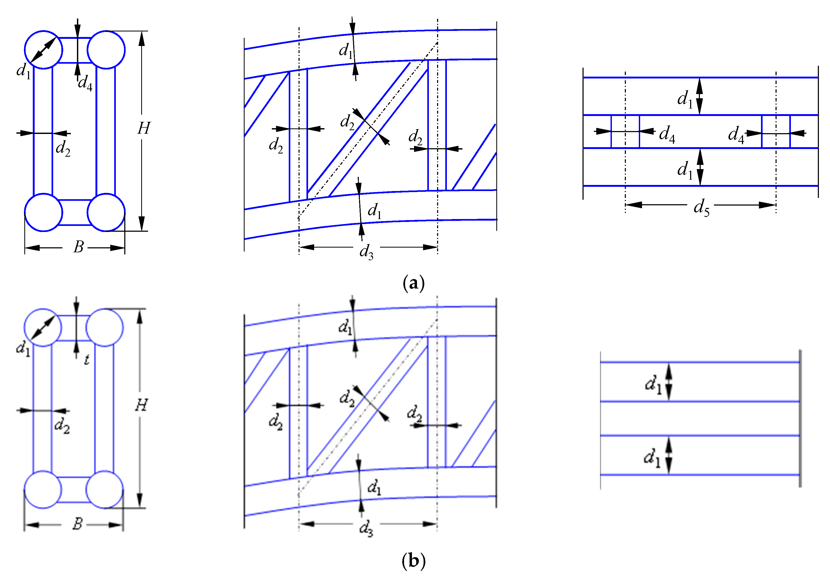
Figure 1. Sections for arch rib models. (a) Four-tube trussed section; (b) horizontal dumbbell trussed section.
Buildings 15 01837 g001
Figure 2. Dimensions of the adopted truss sections. (a) Four-tube trussed section; (b) horizontal dumbbell trussed section.
Buildings 15 01837 g002
Figure 3. Section models of arch rib. (a) FTT model; (b) HDT model.
Buildings 15 01837 g003
Figure 4. Installation of piano wires.
Buildings 15 01837 g004
Figure 5. Influence of piano wires on drag coefficients.
Buildings 15 01837 g005
Figure 6. Variations in drag coefficient with tripwire for different wind speeds.
Buildings 15 01837 g006
Figure 7. Illustration of the tripwires. (a) Layout of tripwires on tubes; (b) layout of tripwires on section models.
Buildings 15 01837 g007
Figure 8. Illustration of the wind tunnel. (a) Wind tunnel at Kyoto University; (b) turntable.
Buildings 15 01837 g008
Figure 9. Illustration of instrumentations. (a) Load cell (LMC-3501); (b) X-type hot wires.
Buildings 15 01837 g009
Figure 10. Illustration of instrumentations.
Buildings 15 01837 g010
Figure 11. Assembled section model in the wind tunnel.
Buildings 15 01837 g011
Figure 12. Aerodynamic force coefficients under laminar flow. (a) FTT-I (B = 67.5 mm); (b) HDT-I (B = 67.5 mm); (c) FTT-II (B = 86.5 mm); (d) HDT-II (B = 86.5 mm); (e) FTT-III (B = 105 mm); (f) HDT-III (B = 105 mm).
Buildings 15 01837 g012
Figure 13. Force coefficients under 0° attack angle.
Buildings 15 01837 g013
Figure 14. Force coefficients tested under turbulent flow. (a) FTT-I (B = 67.5 mm); (b) HDT-I (B = 67.5 mm); (c) FTT-II (B = 86.5 mm); (d) HDT-II (B = 86.5 mm); (e) FTT-III (B = 105 mm); (f) HDT-III (B = 105 mm).
Buildings 15 01837 g014
Figure 15. Power spectrum estimations of model HDT-I. (a) Fluctuating wind speed time series; (b) fluctuating wind speed spectrum; (c) fluctuating drag time series; (d) fluctuating drag spectrum.
Buildings 15 01837 g015
Figure 16. Drag spectrum under laminar flow.
Buildings 15 01837 g016
Figure 17. Relationship between Strouhal number and spacing ratio.
Buildings 15 01837 g017
Figure 18. Fitting of decay factor (λ = 14). (a) x = 0 m, y1 = 0 m, y2 = 0.025 m; (b) x = 0 m, y1 = 0 m, y2 = 0.05 m; (c) x = 0 m, y1 = 0 m, y2 = 0.075 m; (d) x = 0 m, y1 = 0 m, y2 = 0.125 m; (e) x = 0 m, y1 = 0 m, y2 = 0.175 m; (f) x = 0 m, y1 = 0 m, y2 = 0.225 m.
Buildings 15 01837 g018
Figure 19. Experimental equivalent AAF of FTT-I.
Buildings 15 01837 g019
Figure 20. Comparisons between the fitted and test results of equivalent AAF. (a) FTT-I (B = 67.5 mm); (b) HDT-I (B = 67.5 mm); (c) FTT-II (B = 86.5 mm); (d) HDT-II (B = 86.5 mm); (e) FTT-III (B = 105 mm); (f) HDT-III (B = 105 mm).
Buildings 15 01837 g020
Figure 21. Comparison of equivalent AAFs.
Buildings 15 01837 g021
Figure 22. Procedure of buffeting analysis.
Buildings 15 01837 g022
Figure 23. Modal shapes of horizontal suspension cable.
Buildings 15 01837 g023
Figure 24. Finite element model of Shenzhen Rainbow Bridge.
Buildings 15 01837 g024
Figure 25. The first 5 modal frequencies and vibration patterns.
Buildings 15 01837 g025
Figure 26. The buffeting analysis results of the cantilevered arch rib. (a) Joint admittance function; (b) modal force spectrum; (c) dynamic amplification factor; (d) modal displacement spectrum; (e) displacement spectrum; (f) displacement response.
Buildings 15 01837 g026
Figure 27. Effect of different equivalent AAFs on the peak displacement.
Buildings 15 01837 g027
Figure 28. Effect of coherence functions on the peak displacement.
Buildings 15 01837 g028
Figure 29. Comparison of mode shapes and peak displacements. (a) Modal shapes; (b) peak displacement.
Buildings 15 01837 g029
Figure 30. Influence of mode number on the displacement response.
Buildings 15 01837 g030
Table 1. Dimensions of section models (unit: mm).
Section ModelslBHB/Hd1d2d3d4d5t
FTT-I90067.51500.45301515015150-
FTT-II90086.51500.58301515015150-
FTT-III900105.01500.7301515015150-
HDT-I90067.51500.453015150--21
HDT-II90086.51500.583015150--21
HDT-III900105.01500.73015150--21
Table 2. Force coefficients at a 0° attack wind angle in turbulent flow.
Section ModelsB/mmCDCLCM
FTT-I67.51.11−0.04050.0478
FTT-II86.51.24−0.110−0.0203
FTT-III105.01.24−0.0958−0.0435
HDT-I67.50.990.00714−0.0359
HDT-II86.51.100.0375−0.0112
HDT-III105.01.070.0292−0.000732
Disclaimer/Publisher’s Note: The statements, opinions and data contained in all publications are solely those of the individual author(s) and contributor(s) and not of MDPI and/or the editor(s). MDPI and/or the editor(s) disclaim responsibility for any injury to people or property resulting from any ideas, methods, instructions or products referred to in the content.

