Article

Intelligent Optimization Method for Rebar Cutting in Pump Stations Based on Genetic Algorithm and BIM

1
College of River and Ocean Engineering, Chongqing Jiaotong University, Chongqing 400074, China
2
Xinjiang Surveying & Designing Institute of Agriculture Ministry, Urumqi 830002, China
3
School of Civil Engineering, Chongqing University, Chongqing 400044, China
*
Author to whom correspondence should be addressed.
Buildings 2025, 15(11), 1790; https://doi.org/10.3390/buildings15111790
Submission received: 24 April 2025 / Revised: 21 May 2025 / Accepted: 22 May 2025 / Published: 23 May 2025

Abstract

As the construction industry shifts from an extensive development model to one characterized by intelligent structural systems, the imperative to enhance productivity and management efficiency has emerged as a critical challenge. Conventional rebar construction processes heavily rely on manual operations—such as on-site rebar cutting, manual transcription of material lists, and decentralized processing—which are susceptible to subjective errors and often result in significant material waste. This issue is particularly pronounced in large-scale projects, where disorganized management of rebar quantities and placements exacerbates inefficiencies. To address these challenges, this study proposes an integrated approach that synergistically combines a genetic algorithm-based rebar-cutting optimization model with BIM technology, thereby optimizing rebar management throughout the construction process. The research is structured into two primary components. Firstly, a one-dimensional mathematical model for rebar-cutting optimization is developed, incorporating an innovative real-number encoding strategy within the genetic algorithm framework to maximize material utilization. A case study conducted on a pump station project reveals that the utilization rates for 32 mm and 16 mm rebar reach 86.76% and 93.90%, respectively, significantly exceeding the industry standard of 80%. Secondly, an automated batch modeling tool is developed using C# and the Revit API, which enables the efficient generation of rebar components; a unique coding system is employed to establish a bidirectional mapping between the digital model and the physical rebar, ensuring precise positioning and effective information management. Overall, this integrated method—encompassing rebar-cutting optimization, digital modeling, and on-site intelligent management—not only mitigates material waste and reduces production costs but also markedly enhances construction efficiency and accuracy in complex projects, thereby providing robust technical support for the seamless integration of intelligent construction and industrialized building practices.

1. Introduction

Rebar, as one of the three primary materials in construction, constitutes a substantial portion of total project costs. Traditional rebar operations—cutting, bending, and installation—rely heavily on manual labor and are thus vulnerable to human error, miscalculations, and inexperience, leading to considerable material waste. In large-scale pumping station projects, the complexity of the structural design exacerbates this inefficiency. Additionally, the high volume of rebar and intricate layout during installation phases often result in information ambiguity and positional confusion, contributing to disorganized planning and ineffective site management. With the ongoing shift toward digitalization in the construction industry, rebar management is evolving from labor-intensive to data-driven and precision-oriented practices. By integrating an optimized rebar-cutting model based on an enhanced genetic algorithm with Building Information Modeling (BIM), intelligent rebar processing can be achieved. This approach not only minimizes material waste and production costs, but also improves the efficiency and accuracy of on-site construction workflows.

1.1. Intelligent Optimization of Rebar Cutting

The rebar-cutting stock problem (CSP) was first introduced by Soviet mathematician Kantorovich in 1939 as a discrete allocation model with binary and integer variables under stock constraints [1]. However, the model exhibited two major drawbacks: a weak continuous relaxation and a large number of symmetries caused by permutations. To overcome the limitations of the original formulation, Gilmore and Gomory proposed a linear programming model based on the knapsack problem. They further developed the delayed column generation technique, which improves efficiency by reducing redundant computations while preserving solution accuracy [2,3]. This approach has since served as a foundation for solving more complex CSP variants with multiple lengths and constraints [4,5].
Due to the difficulty of simultaneously achieving integrality and optimality, heuristic algorithms have been widely adopted as effective approximation techniques [6,7]. Among these, Haessler et al. developed the Haessler model, which aims to minimize raw material waste and employs a Sequential Heuristic Procedure (SHP) for solution construction [8,9]. SHP first determines the optimal cutting pattern for a single stock unit using dynamic programming, and then iteratively builds the overall cutting plan. While efficient, SHP is highly sensitive to item ordering and often converges to suboptimal solutions [10,11]. To mitigate these shortcomings, Belo and Scheithauer introduced the Sequential Value Correction (SVC) framework [12]. This method dynamically assigns value scores to individual items based on the current utilization rate or trim loss. After each SHP iteration, item values are updated, and the procedure is repeated. The SVC–SHP approach improves search robustness by enabling escape from local optima and gradually converging to higher-quality solutions while maintaining the simplicity and efficiency of SHP [13,14].
With the increasing complexity and scale of engineering projects, traditional heuristics face limitations in scalability and performance [15]. As a result, recent research has focused on intelligent optimization algorithms. Onwubolu was among the earliest to apply genetic algorithms (GAs) to the CSP, demonstrating clear advantages in both solution quality and convergence rate compared to classical heuristics [16]. Building on this, Gracia et al. developed a hybrid GA by integrating additional search and clustering strategies into the standard GA framework, further enhancing performance [17]. In addition to GA-based approaches, other AI-driven methods have also been explored. Kang applied neural networks to the CSP and achieved promising outcomes, highlighting the feasibility of machine learning in cutting optimization [18]. Jahromi compared simulated annealing (SA) and tabu search (TS) for large-scale instances and found that SA offered superior performance in both convergence speed and solution quality, emphasizing the importance of balancing global and local search strategies [19]. Furthermore, Bressan proposed a tree-based heuristic algorithm that effectively reduced material usage and cut time, contributing to cost savings in industrial operations [20]. Fang et al. proposed a deep reinforcement learning (DRL)-based algorithm that effectively reduced raw material consumption and enhanced solution generalization across various instances, demonstrating significant potential for industrial applications [21]. Barragán-Vite et al. introduced a Petri net-based algorithm utilizing a filtered beam search strategy, which efficiently identified optimal and near-optimal solutions for both low and high-complexity instances of the 1D-CSP [22]. Martin et al. developed a pattern-based integer linear programming (ILP) model that simultaneously minimizes the number of stock objects and cutting patterns, addressing setup costs and providing exact solutions for moderate-sized instances [23].
Building upon these advancements, this study adopts a genetic algorithm (GA) to model and optimize the rebar-cutting stock problem, owing to several notable advantages. First, GA exhibits strong global search capabilities, making it well-suited for complex engineering optimization tasks characterized by large solution spaces, nonlinear constraints, and multiple objectives. Second, GA is problem-agnostic and does not require gradient information or explicit mathematical formulations, allowing flexible integration of practical constraints. Third, in response to the continuous nature of rebar lengths, this study introduces a real-number encoding strategy to enhance the precision of solution representation. Additionally, a multi-objective fitness function is designed to account for both trim loss and leftover utilization, thereby improving interpretability and optimization effectiveness. Compared to traditional heuristics, the proposed GA-based method demonstrates superior performance in terms of solution quality, efficiency, and scalability, making it particularly suitable for large-scale construction projects involving diverse rebar types and complex component geometries.

1.2. BIM-Assisted Construction Technologies

In the late 20th century, Professor Adjei-Kumi of the University of Strathclyde was among the first to introduce Building Information Modeling (BIM) into construction schedule management, aiming to address the limitations of the PROVISYS model in project planning [24]. With the advancement of computing power and iterative improvements in software, BIM has gradually evolved from a design tool into a collaborative platform that supports multiple project phases and stakeholders [25,26]. For instance, Sacks et al. conducted in-depth studies on BIM-based information integration and coordination in construction processes, promoting its application in construction automation and prefabrication design workflows [27]. Succar proposed the BIM Maturity Matrix, offering a structured framework for evaluating BIM implementation across design, construction, and facility management stages [28]. Hartmann et al. explored the application of 4D BIM in construction scheduling, simulation, and progress control, highlighting its roles in visualization, coordination, and decision support on construction sites [29].
While these studies have significantly advanced BIM-based project and safety management, relatively little attention has been paid to on-site material management. In response to challenges such as the low level of digitalization and fragmented management practices in this area, Toyin et al. evaluated BIM’s potential as a material management tool, concluding that it can effectively reduce rebar waste and optimize supply chain operations [30]. Lee et al. proposed a BIM-based construction information management framework, which structures site-generated documentation and links it to BIM models, enabling information visualization and knowledge retention during the construction phase [31]. Bortolini et al. developed a 4D BIM-based logistics planning and control model for Engineer-to-Order (ETO) prefabricated systems, facilitating real-time coordination of on-site logistics with BIM workflows [32].
As BIM continues to penetrate the full lifecycle of construction projects, standardized software platforms are increasingly insufficient to meet the diverse and dynamic needs of modern construction management. Consequently, recent research and industry practices have focused on the secondary development of BIM platforms, aiming to enhance their practicality and intelligence in managing on-site materials, logistics coordination, and progress tracking.
Currently, while there have been studies on rebar-cutting optimization or BIM-assisted construction management, successful cases that deeply integrate genetic algorithm-based optimization models with BIM platforms to achieve intelligent generation and query management of rebar-cutting plans are still relatively scarce. This paper covers the entire process from rebar-cutting optimization and digital modeling to on-site intelligent management, effectively reducing material waste and production costs, while significantly improving the construction efficiency and accuracy of complex building projects. It provides strong technical support for the deep integration of smart construction and industrialization of the construction sector.

2. Rebar-Cutting Optimization Model for Pump Station Based on an Improved Genetic Algorithm

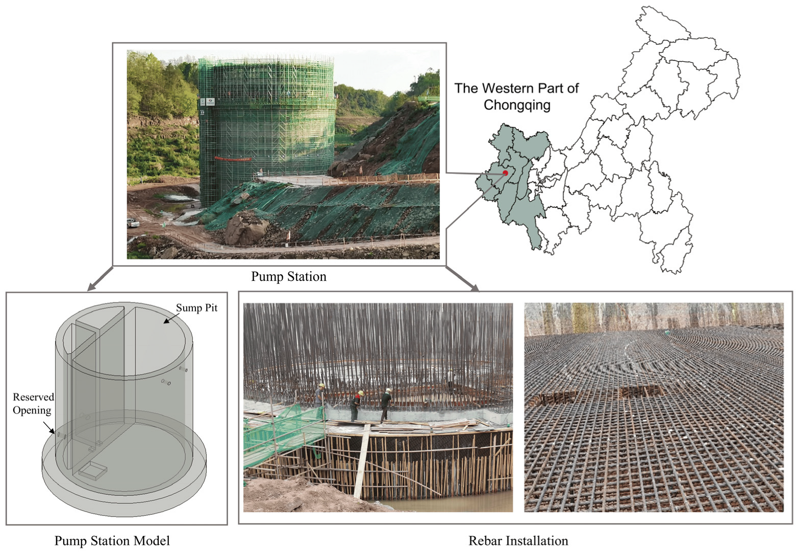
2.1. Rebar Detailing for the Pump Station

As shown in Figure 1, this study selects a pump station from the western route of the YuXi Water Diversion Project as a practical case. The pump station features a cylindrical structure with a circular base measuring 24 m in diameter and an overall height of 23.6 m. The maximum length of vertical rebars reaches 16.85 m, while horizontal rebars can extend up to 28.8 m. Considering the actual construction conditions, vertical concrete pouring is conducted in multiple lifts, each constrained by a fixed formwork height of 3 m. Consequently, the vertical rebars must be segmented accordingly in compliance with relevant construction standards. The available rebar lengths on-site are 9 m and 12 m. Since some horizontal rebar segments exceed these lengths, mechanical splicing sleeves are required to meet design specifications.

2.1.1. Pump Station Sidewall

The pump station has an overall height of 23.6 m. Vertical rebars along the internal sidewalls must be segmented and tied in accordance with the pouring sequence. According to the Technical Specification for Construction of Hydraulic Concrete (SL 677–2014), the outer structure of the pump station is subjected to long-term hydrostatic pressure during operation, and the vertical rebars experience combined tension and compression. The minimum lap splice length is specified as 40 times the bar diameter. For the commonly used diameters of 25 mm and 32 mm, this corresponds to lap lengths of 1000 mm and 1280 mm, respectively. To facilitate field operations, lap lengths of 1000 mm and 1300 mm were ultimately adopted.
Based on the required bar lengths, the vertical rebars are categorized into four types: 14.55 m, 15.85 m, 8.9 m, and 10.2 m. The sidewall construction is divided into eight lifts. Excluding the overlap with the base slab, each lift has an approximate height of 3 m. Lap splices between adjacent segments must be staggered vertically to avoid alignment. The segmentation layout of the rebars, as derived from this constraint, is illustrated in Figure 2.
According to the segmentation pattern, the rebars are divided into eight vertical sections from bottom to top. The final segmentation arrangement is summarized in Table 1. Some rebars, such as rebar types 2-4 and 3-4, are L-shaped. For instance, a designation of 300 + 100 indicates a 300 cm vertical segment with a 90° bend segment of 100 cm.
After compiling all segment types and quantities, a summary of rebar-cutting requirements for the sidewall is generated, as shown in Table 2.

2.1.2. Pump Station Bottom Slab

According to the design drawings, the bottom reinforcement of the pump station slab is arranged in a cross pattern. The steel bars are numbered based on their linear distance from the centerline, with the steel bar positioned at the centerline assigned number 1. The further the steel bar is from the centerline, the higher the number assigned. The length lll of each steel bar in the plane is calculated as follows:
l = 2 L 2 d 2
In the equation, L has a constant value of 12.05 m, which is the radius of the pump station slab minus a 5 cm protective layer; and d represents the distance from the centerline to the position of each rebar.
The diameter of all steel bars in the pump station slab is 32 mm. According to the design specifications, the minimum mechanical connection spacing between adjacent bars is 35 times the diameter of the steel bars, resulting in a minimum distance of 1.12 m. To minimize the number of couplers used, the reinforcement is preferably arranged using complete lengths of 12 m, 9 m, and new cut lengths. In order to ensure that the coupler positions are staggered and the minimum distance is greater than 1.12 m, the steel bars are arranged in a staggered layout. The final arrangement of the steel bar splices is shown in Table 3.
The arrangement of top rebars in the pump station base slab is generally similar to that of the bottom layer. However, the presence of three sump pits at the bottom causes slight adjustments to some rebar positions. The splicing layout of the top rebars is detailed in Table A1, and the final overall reinforcement layout of the base slab is illustrated in Figure 3.

2.2. Improved Genetic Algorithm for the Cutting Stock Problem

2.2.1. Mathematical Model of the Cutting Stock Problem

The one-dimensional cutting stock problem is a classical combinatorial optimization problem. The objective is to cut raw materials of fixed lengths into a set of parts of specified types and lengths while determining the cutting patterns and their frequencies. Depending on the optimization goal, the problem can be categorized into two types: minimizing the total number of raw material bars used or maximizing material utilization. Considering the actual construction conditions at the pump station site, a mathematical model is established with a dual specification of raw material lengths: 9 m and 12 m. The optimization objective is to maximize raw material utilization.
Assume there are two types of raw material lengths, the following defines all the sets, parameters, and decision variables along with their types and units. The model parameters are summarized in Table 4.
(1) Sets and parameters
L x and L y : Two types of raw material lengths, in meters (m).
q : The number of required part types.
l k ( k = 1 , 2 , , q ): The length of the k t h part, in meters (m).
a k ( k = 1 , 2 , , q ): The demand for the k t h part, in pieces (pcs).
m   ( n ): The number of cutting patterns for raw material L x ( L y ).
x k i : The number of the k t h part in the i t h cutting pattern, in pieces (pcs).
y k j : The number of the k t h part in the j t h cutting pattern, in pieces (pcs).
b i ( c j )   : The trim loss for the i t h ( j t h ) cutting pattern, in meters (m).
(2) Decision variables
X i   : The frequency of the i t h cutting pattern, in pieces (pcs).
Y j : The frequency of the j t h cutting pattern, in pieces (pcs).
The objective function is to maximize the material utilization:
max z = k = 1 q l k · a k i = 1 m X i · L x + j = 1 n Y j · L x
The total number of parts produced meets the required demand:
i = 1 m X i · x k i + j = 1 n Y j · y k j a k
Cutting pattern feasibility constraints are as follows:
k = 1 q l k · x k i L X
k = 1 q l k · y k j L Y
Trim loss for each pattern is calculated as follows:
b i = L X k = 1 q l k · x k i
c i = L Y k = 1 q l k · y k j

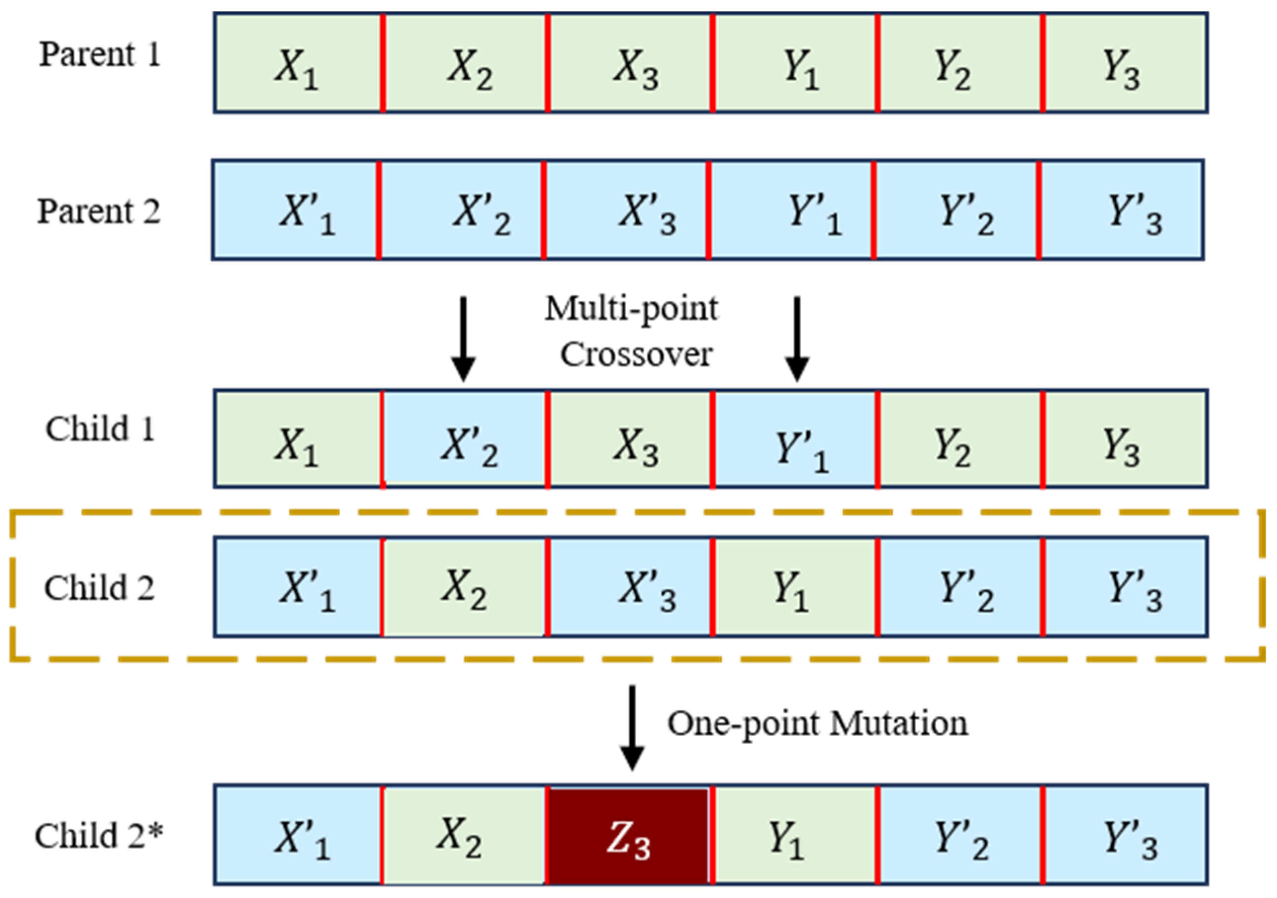
2.2.2. Genetic Algorithm Improvement

To solve the mathematical model of the one-dimensional cutting stock problem established above, a genetic algorithm (GA) is employed. Considering the practical needs of engineering applications, a real-number encoding strategy is adopted to address the dual-length raw material cutting issue. The overall procedure is illustrated in Figure 4.
Step 1: Initialization of basic parameters
Input all known data, including the lengths of available raw materials, the required part lengths, and the corresponding quantities. Set the basic parameters of the algorithm, including the population size, the number of iterations, the crossover probability, and the mutation probability.
Step 2: Encoding strategy
For each individual in the population, a real-number encoding strategy is defined based on the number of cutting patterns. The chromosome is composed of two parts: cutting patterns based on the length L x are placed at the beginning, followed by those for L y . Each position in the chromosome represents the number of repetitions of a specific cutting pattern. All cutting patterns are indexed as {1, 2, …, m, 1, 2, ..., n}, with a total chromosome length of m + n , corresponding to repetition counts { X 1 , X 2 , , X m , Y 1 , Y 2 , , Y n } . To improve computational efficiency, the maximum repetition count Q is predefined based on the highest frequency among all feasible cutting patterns, and each gene value is randomly initialized within the range 0 , Q . For example, a chromosome such as {4, 7, 9, …, 8} indicates that the first cutting pattern is repeated 4 times, the second pattern 7 times, the third 9 times, and so on, up to the final Y n pattern with 8 repetitions.
Step 3: Cutting pattern generation
Based on the encoding strategy, all feasible cutting patterns are enumerated. To ensure high material utilization, each cutting pattern must yield a trim loss smaller than the shortest required part length l m i n . Patterns are computed separately for both lengths L x and L y . The results are stored in two matrices, detailing the number of parts of each type obtained from every cutting pattern, along with the resulting waste.
Step 4: Population initialization
Based on the encoding rule in Step 2, an initial population is randomly generated. Each chromosome has a length of m + n , with gene values ranging from 0 to Q . The population size is determined by the algorithm’s predefined parameters.
Step 5: Fitness evaluation
The fitness function is defined based on the raw material utilization rate. A higher utilization rate corresponds to higher fitness. The maximum fitness value is 1, indicating full utilization. If a chromosome fails to satisfy the required number of parts, a penalty mechanism is applied: the fitness value is set to −1, and the chromosome is replaced with a newly generated one in the next iteration. The fitness function is defined as follows:
max z = k = 1 q l k · a k i = 1 m X i · L x + j = 1 n Y j · L x , i = 1 m X i · x k i + j = 1 n Y j · y k j a k 1 , i = 1 m X i · x k i + j = 1 n Y j · y k j < a k
Step 6: Selection of Individuals
A roulette wheel selection method is adopted to select high-fitness individuals from the current population to form the parent population for the next generation. This probabilistic selection is based on each individual’s fitness value. The process is described in the Algorithm 1:
Algorithm 1. Selection
Input:Population and corresponding fitness values
1:Calculate the total fitness of all individuals in the current population.
2:For each individual, compute its selection probability as its fitness divided by the total fitness; construct the basic roulette wheel accordingly.
3:For  i = 1 to population size, do:
4:Generate a random number p i c k uniformly in the interval ( 0,1 ) .
5:Starting from the first individual, accumulate the selection probabilities until the sum exceeds p i c k . The individual at this point is selected.
6:End for
Output:New population after selection.
Step 7: Crossover Operator (Algorithm 2)
Two individuals are randomly selected from the population to perform crossover operations. A multi-point crossover strategy is adopted, where gene segments between selected points are exchanged to generate two new offspring. This process aims to inherit advantageous traits from the parent chromosomes, thereby enhancing the optimization of the population. A schematic diagram of multi-point crossover is shown in Figure 5.
Algorithm 2. Crossover
Input:Population and crossover probability
1:For  i = 1 to population size, perform crossover operations equal to the population size.
2:Randomly select two individuals to serve as parents.
3:Generate a random number p i c k   ( 0 ,   1 ) and compare it with the crossover probability:
 - If p i c k < crossover probability: skip crossover, return to step 1.
 - If p i c k   crossover probability: continue with crossover.
4:Randomly generate two integers a , b [ 2 , m + n 1 ] , and sort them so that b > a . The interval   [ a , b ] is used as the crossover range.
5:Exchange the gene segments between the two parents within the [ a , b ] range.
6:End for
Output:Population after crossover.
Step 8: Mutation Operator (Algorithm 3)
To maintain population diversity and prevent premature convergence, mutation is performed by randomly selecting an individual and altering one of its gene positions.
Algorithm 3. Mutation
Input:Population and mutation probability
1:For  i = 1 to population size, perform mutation operations equal to the population size.
2:Randomly select one individual for mutation.
3:Generate a random number p i c k   ( 0 ,   1 ) and compare it with the mutation probability:
 - If p i c k < mutation probability: skip mutation, return to step 1.
 - If p i c k   mutation probability: continue with mutation.
4:Randomly generate an integer a [ 1 , m + n ] , representing the gene position to be mutated.
5:Determine the maximum allowable value Q for this gene, then generate a random integer   b 0 , Q   and replace the gene at position aaa with b .
6:End for
Output:Population after mutation.
Step 9: Final Output
After completing all iterations, the individual with the highest fitness value in the final population is selected as the optimal solution. A graph depicting the evolution of fitness values over iterations is also generated to illustrate convergence.

3. Development of Rebar Batch Generation and Query Components

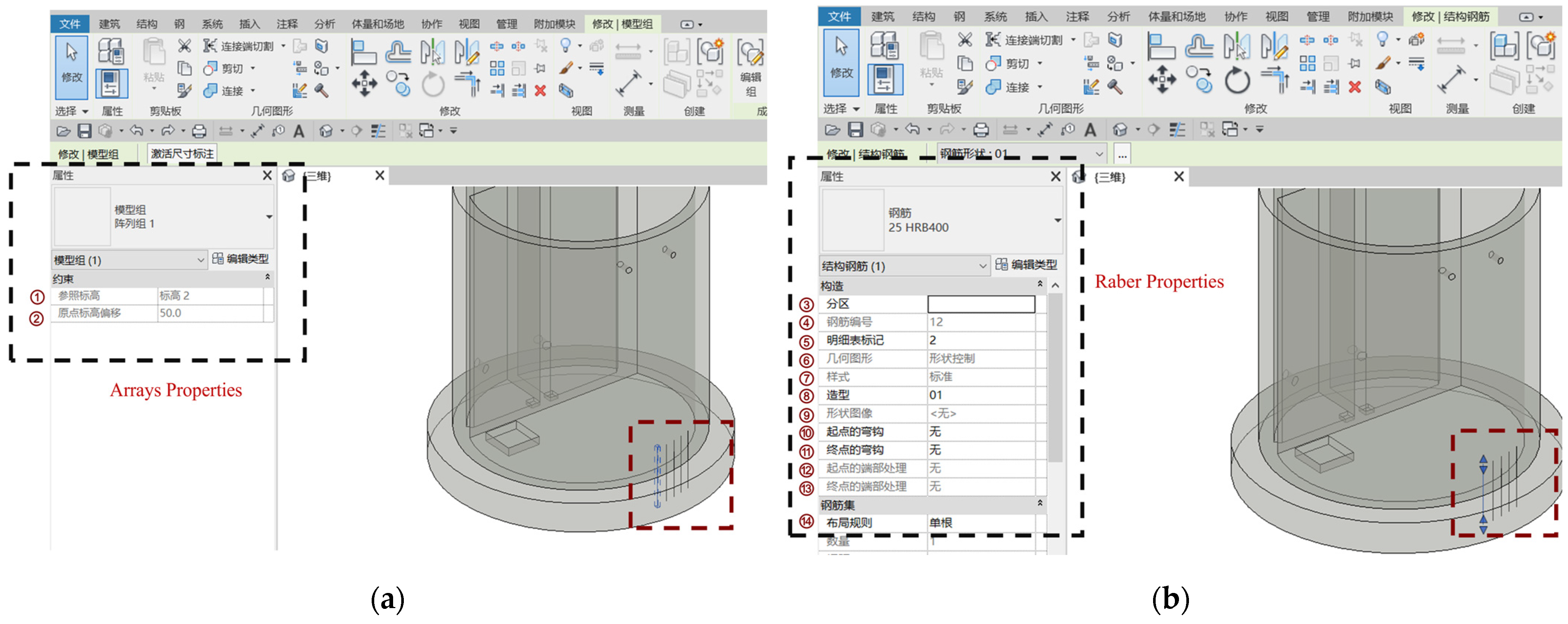
3.1. Rebar Batch Generation via Revit Secondary Development

Revit secondary development refers to the use of Revit’s API (Application Programming Interface) for custom development, allowing users to extend or enhance the native functionalities of Revit. In this section, by customizing the Revit API and integrating the rebar arrangement tables and diagrams calculated in Section 2, various types of rebars used during the construction phase are automatically generated within the pump station model. This enables batch creation of rebar elements, significantly simplifying the repetitive tasks involved in the modeling process. Revit 2020 and Visual Studio 2019 were used as the development platforms, with C# as the programming language. The project was created using the “Class Library (.NET Framework)” template and configured to target .NET Framework 7.
There are three primary methods for creating rebar elements through the Revit API:
  • R.CFRS—Creation based on existing system rebar shapes;
  • R.CFC—Creation based on custom curves;
  • R.CFCAS—Creation based on rebar shape curves.
According to the location and type of rebar in the pump station, they are categorized into sidewall rebars, base slab rebars, and general stirrups. Based on the design drawings, there are three types of general stirrups, which can be created using the R.CFC method.
Since the pump station is a cylindrical structure, the vertical rebars of the sidewall are distributed along arcs. The R.CFRS command is used to generate basic rebar instances, and then the Array Anchor Member command is called to set the angular spacing. The rebars are subsequently ungrouped as a batch via code to allow direct access and modification of their properties. According to Table 1, rebars with arc-shaped distribution include types 2-3, 2-4, and 2-5. The encoding system follows a pattern: the first four digits correspond to the drawing number, the fifth digit indicates the arrangement group, and the last digit specifies the segment order. For instance, a rebar with drawing number 2-3, diameter 32 mm, total length 8.9 m, and cut length 2.45 m is encoded as 020311.
Base slab rebars are created using the R.CFC method. Full layout is achieved through duplication and rotation via code. The encoding method for base slab rebars slightly differs from that of vertical rebars: the first four digits still refer to the drawing number, while the last two digits correspond to the rebar position in the diagram. For example, 010303 denotes the third rebar in the group with drawing number 1-3.

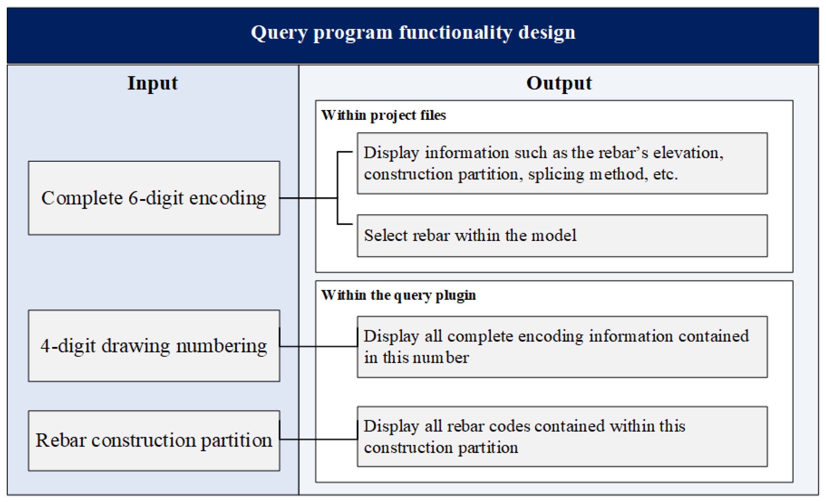
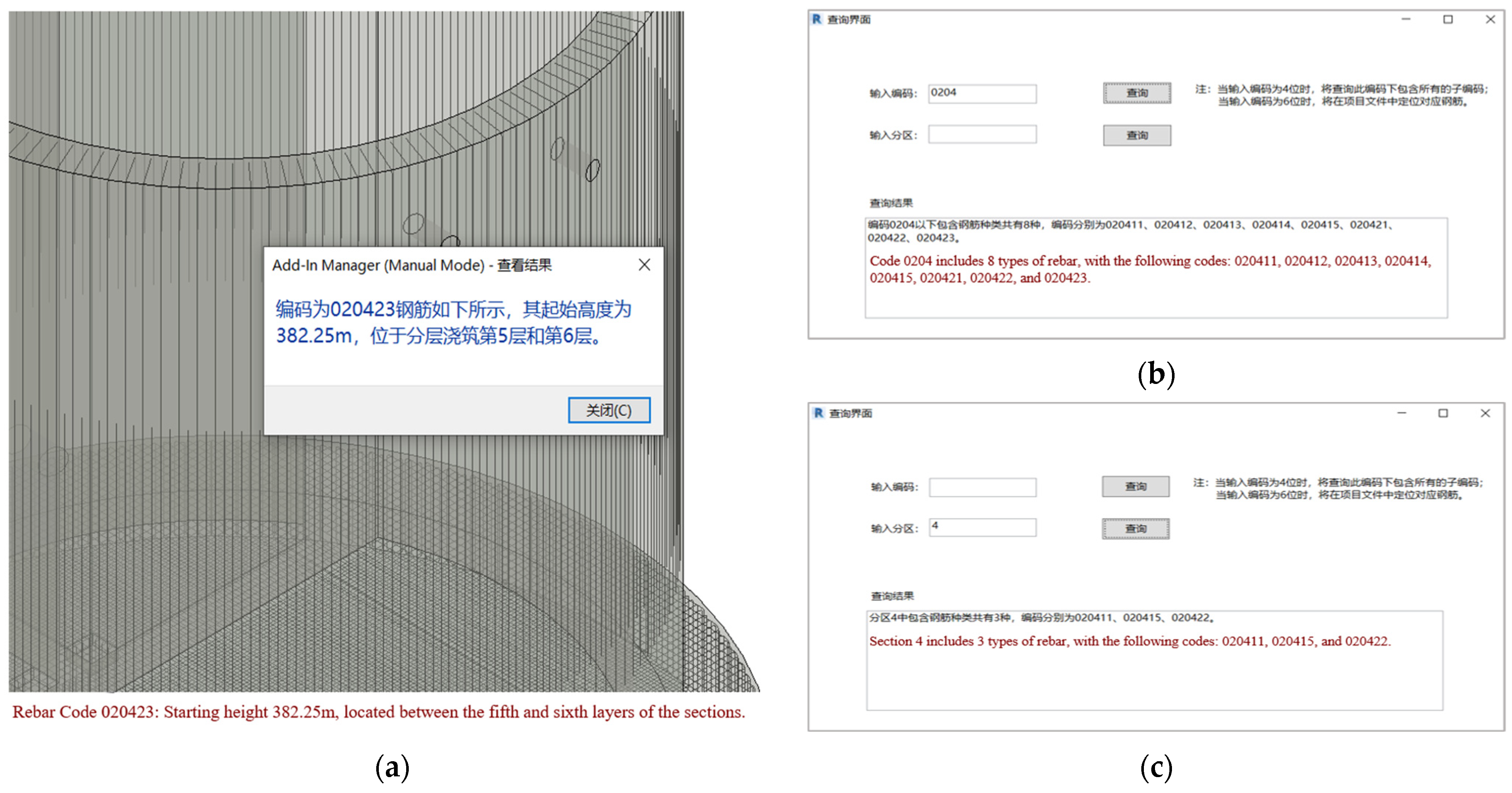
3.2. Development of Rebar Query Component

To address challenges such as information overload and positional confusion caused by a large number of rebar elements during construction, this section presents a rebar query module. For all rebar instances created in the pump station model, corresponding codes and annotation data are added. A query interface is developed using the WPF framework, allowing users to search for specific rebar information—such as position, segment length, and elevation—based on the rebar code. This bidirectional link between the model and the physical construction site facilitates intelligent rebar management during construction. As shown in Figure 6, the query program provides three different search modes:
  • Query by first four digits of the code: returns all rebars under the same drawing number, allowing for specific individual queries.
  • Query by full six-digit code: selects the corresponding rebar element in the document and displays its annotation.
  • Query by partition: returns all rebar codes contained within a given zone.
To ensure seamless interaction with Revit and maintain clean code architecture, the development follows the Single Responsibility Principle. Functional logic is separated from the main WPF window class (MainWindow.xaml.cs). Additional class files are introduced to handle launching the WPF application from within Revit and executing the actual query commands. The relationships among these files are illustrated in Figure 7.

4. Results

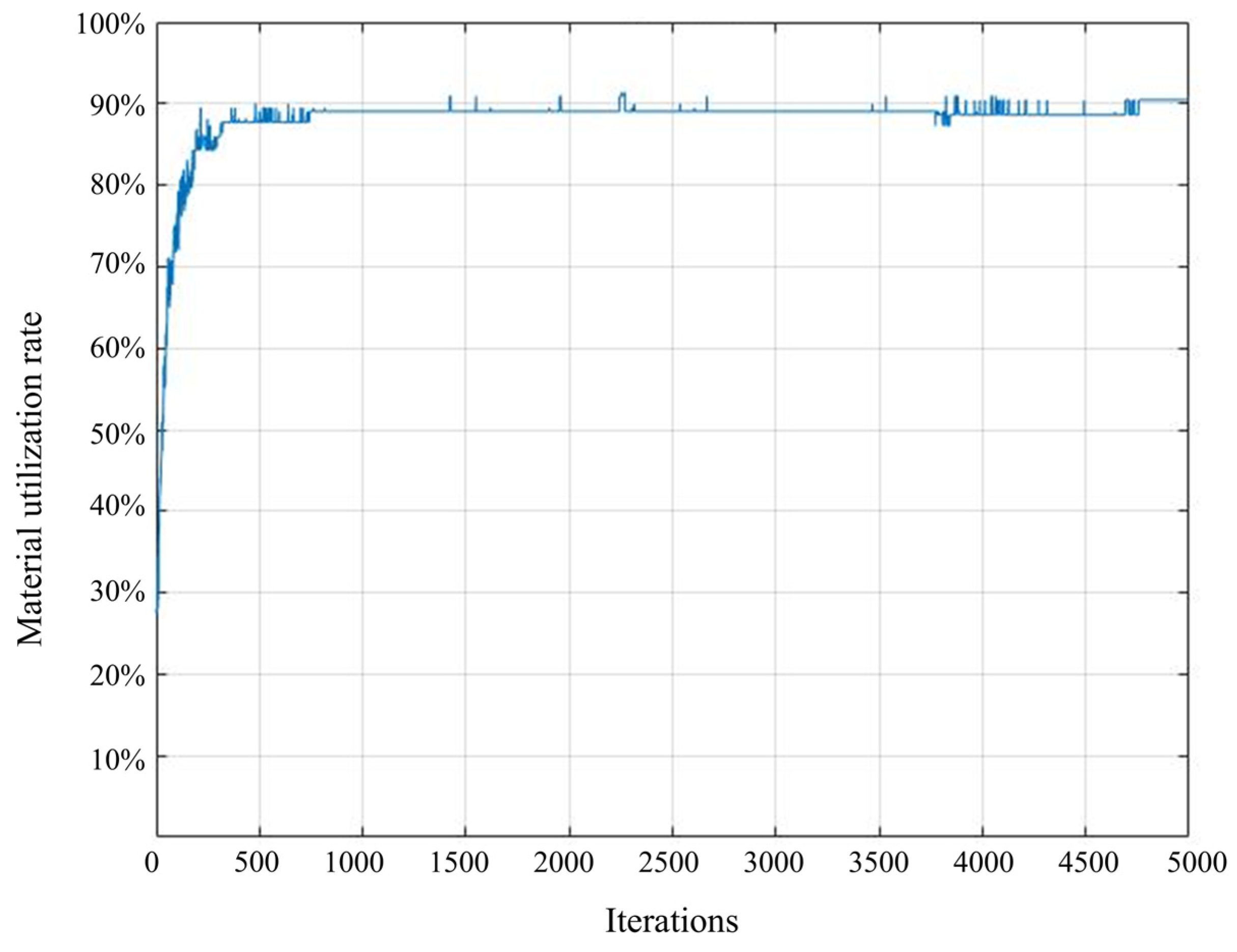
4.1. Optimization Results of the Improved Genetic Algorithm

Taking the 16 mm rebar used in the pump station as an example, a total of 24 cutting patterns were generated, including 9 patterns based on 9 m raw materials and 15 patterns based on 12 m raw materials. In the genetic algorithm implementation, the population size was set to 200, the number of generations to 5000, the crossover probability to 0.9, and the mutation probability to 0.09 [33]. The algorithm was executed 10 times to assess stability and robustness. The best solution achieved a material utilization rate of 93%, which was consistently reached in 8 out of 10 runs. The average utilization rate across all runs was 93.6%, indicating strong convergence and solution quality. The iterative optimization process is shown in Figure 8, where convergence was reached at iteration 315 and maintained until the end.
The final results show that the required quantities for rebar lengths of 5.56 m, 3.12 m, and 2.78 m were fully met, with only one surplus piece of 3.37 m rebar. According to this method, the final material utilization rate reached 93.90%. The detailed cutting plan is shown in Table 5.
Similarly, for the 32 mm rebar, a total of 33 cutting patterns were generated, including 12 patterns based on 9 m raw materials and 21 patterns based on 12 m raw materials. In this case, the population size was set to 3000, the number of generations to 10,000, the crossover probability to 0.99, and the mutation probability to 0.11. The genetic algorithm was executed 10 times to evaluate performance consistency. The best result yielded a material utilization rate of 86%, which was achieved in 7 out of 10 runs. The average utilization rate across all runs was 85.7%, indicating good convergence and robustness of the optimization process. The iterative progression is shown in Figure 9, where the utilization rate stabilized at 86% by generation 4276 and remained unchanged thereafter.
The final cutting results show that the required quantities for rebar lengths of 2.45 m and 4.35 m were completely satisfied, with a surplus of one piece each for the 3.75 m and 4.7 m rebar. Using this optimized method, the final material utilization rate reached 86.76%. The finalized cutting plan is presented in Table 6.

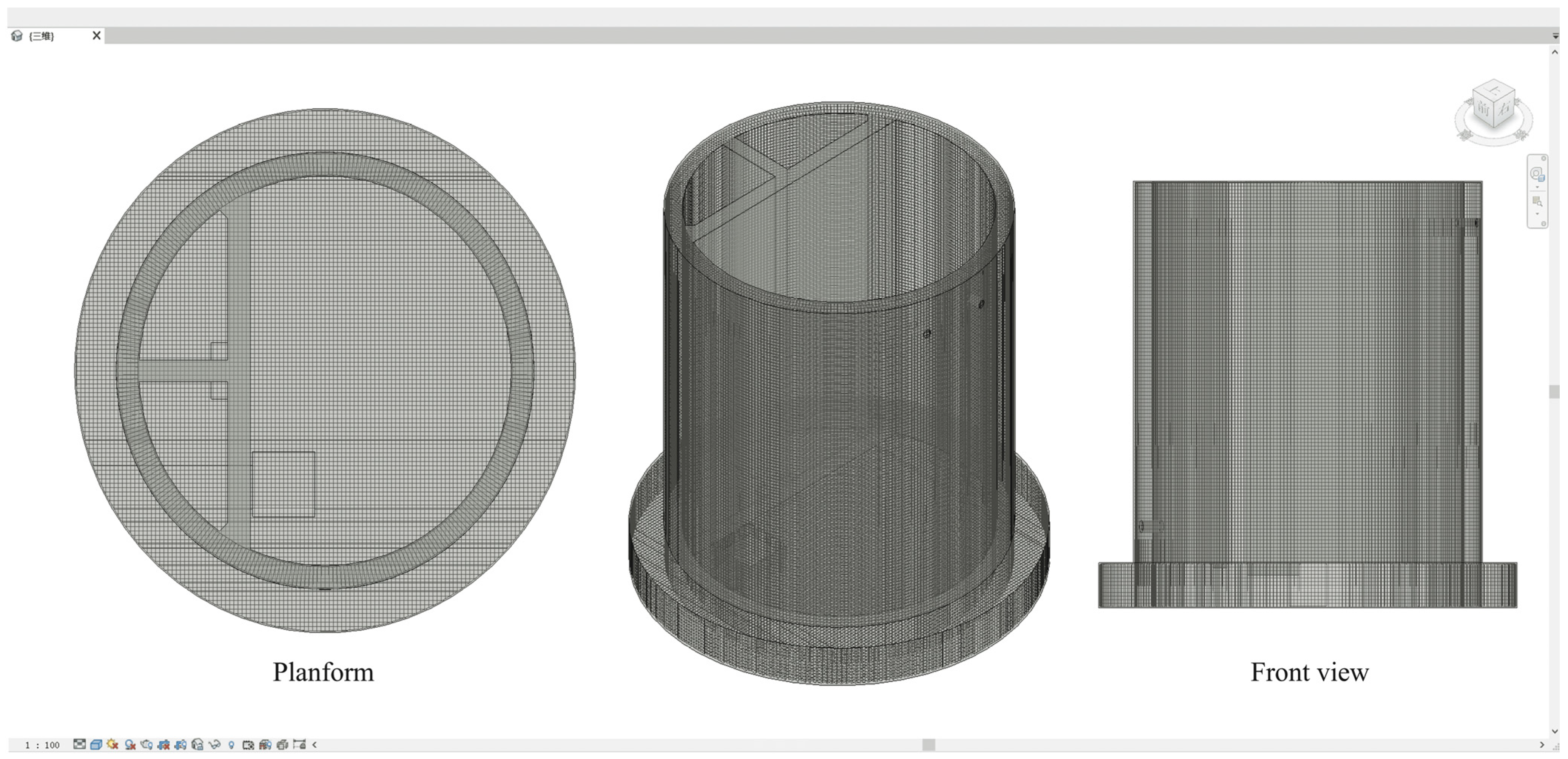
4.2. Application Example of Batch Rebar Generation

Before creating rebar instances, the current Document and the host Family Instance, to which the rebars are attached, must first be accessed through the Revit API. To simplify data entry, the E P P l u s package is used to import Excel data, extracting parameters of types such as int, string, and double for subsequent configuration of rebar parameters.
For the rebar in the pump station’s sidewalls, after generating the base rebar instance, an array function is applied to achieve the curved distribution of rebars. The rebar elements are then ungrouped in batch through code, allowing direct access and modification of their properties. The property table after ungrouping is shown in Figure 10, and a total of 4800 sidewall rebars are established.
For the bottom slab, rebar lengths exceed the available standard rebar lengths, necessitating the use of mechanical couplers for splicing. The bottom slab rebar layout is divided into top and bottom layers. After generating the rebar in the bottom layer, the elements are duplicated and rotated 90° to complete the full layout. However, due to the presence of sump pits on the top layer, the rebar arrangement requires individualized placement; thus, each rebar’s length and position must be pre-calculated. Based on the rebar layout drawings and positional indexing introduced in Section 2, a total of 537 rebars are generated for the bottom slab. Representative parameters of the top slab rebars are provided in Table 7.
The overall stirrups used in the pump station, categorized into three types, are created using the R.CFC method. A total of 223 stirrups are instantiated. Their associated parameters, including elevation and radial distance, are detailed in Table 8.
As shown in Figure 11, a total of 5560 rebar elements were generated in the model using the custom-developed program. All required rebars in both the bottom slab and sidewalls were successfully instantiated. Each rebar was assigned a unique identification code based on its position and function, laying the groundwork for subsequent integration with the rebar query system.

4.3. Application of Rebar Query Component

In this section, a WPF-based rebar query application is developed within Visual Studio, tailored for the pump station model. Recognizing the complexity and high density of rebar elements in construction workflows, the tool enhances management by linking key attributes—such as rebar position, segmentation length, and elevation—between the BIM model and the actual construction site. These annotations improve traceability and reduce errors due to information overload or positional confusion during rebar installation.
For sidewall rebars, additional metadata is assigned to support layered concrete pouring operations, including partitioning information and the initial elevation of each rebar group. As shown in Figure 12, the sidewall is divided into eight vertical zones, each tagged to facilitate structural inspection and progress tracking prior to concrete placement.
The application interface is structured with two input fields—one for rebar code and another for zone number—and a single output panel that displays query results. A query button (Button) is added to initiate the search, and Label controls provide guidance and context for the user, as shown in Figure 13.
The query system supports both 4-digit and 6-digit codes, handled by an if statement that evaluates the input length and routes to the appropriate processing logic. For 6-digit codes, the application iterates through a Revit collector to locate the exact rebar by matching its code, storing the result in an elementList. For 4-digit codes or zone queries, the logic filters rebars by prefix or partition attribute, also storing unique entries in the elementList. To eliminate duplicates in the output, a combination of HashSet and List is employed to ensure distinct codes are displayed. The final UI and query results are illustrated in Figure 14.

5. Conclusions and Future Prospects

This study presents a deeply integrated approach that combines a genetic algorithm-based rebar-cutting optimization model with Building Information Modeling (BIM) technology, aiming to enhance the intelligence and precision of rebar management throughout the entire construction process. The proposed method not only effectively reduces material waste and production costs, but also significantly improves construction efficiency and accuracy for complex architectural projects. Ultimately, this approach provides a robust technical foundation for the convergence of intelligent construction and industrialized building practices. The main contributions and findings are summarized as follows:
  • A one-dimensional rebar-cutting optimization model was developed, incorporating a novel real-number encoding strategy within the genetic algorithm framework. Using a pump station project as a case study, the proposed method successfully maximized material utilization. The results demonstrated a rebar utilization rate of 86.76% for 32 mm rebars and 93.90% for 16 mm rebars—significantly higher than the actual utilization rate of 78% observed in the project.
  • Leveraging Revit-based secondary development, a total of 5560 rebar elements were generated for the bottom slab and sidewalls of the pump station through one-click automation. Each rebar was assigned a unique identifier, establishing a bidirectional link between the digital model and physical construction elements. This ensured accurate rebar placement and facilitated information-driven construction management throughout the project lifecycle.
This research proposes a new encoding strategy tailored to one-dimensional cutting problems, enabling effective optimization of rebar-cutting plans. Depending on part distribution, the cutting problem can be categorized into two types: parts with few specifications and high quantities, and parts with numerous, nearly non-repeating specifications. In the pump station case, due to the relatively limited rebar types, all possible cutting schemes could be efficiently enumerated and optimized using a custom encoding scheme. However, when dealing with more diverse part types, the number of possible cutting combinations increases exponentially, leading to potential redundancy and complex management. To address this challenge, future research may explore the introduction of filtering mechanisms to retain only high-efficiency cutting plans that cover all required rebar types. This would ensure construction completeness while reducing computational scale and further improving material utilization.

Author Contributions

Conceptualization, X.F. and K.J.; methodology, X.F. and Q.X.; software, Y.Z.; validation, K.J., Y.Z. and J.H.; formal analysis, K.J.; investigation, J.H.; data curation, Y.Z.; writing—original draft preparation, Y.Z. and Q.X., writing—review and editing, K.J.; funding acquisition, Q.X. All authors have read and agreed to the published version of the manuscript.

Funding

Supported by the Major Science and Technology Project of Guangxi: Research on Key Technologies for Lean Construction of the Pinglu Canal (Project No: Guike AA23062023). Supported by the Chongqing Municipal Housing and Urban-Rural Construction Committee: Digital Construction Technology of Prefabricated Structures for Extra-large Integrated Hub Stations (Project No: Chengkezi 2023.3−15). Funded by the Chongqing Science and Technology Commission, ID: CSTB2023NSCQ-MSX1082.

Data Availability Statement

The raw data supporting the conclusions of this article will be made available by the authors upon request.

Conflicts of Interest

The authors declare no conflicts of interest.

Appendix A

Table A1. Parameters of Top Slab Reinforcement at the Bottom Slab Area.
IDPosition CodeTotal Length (m)Bending Length 1 (cm)Part 1 (m)Part 2 (m)Bending Length 2 (cm)Quantity
1-4420.062358.06121931
520.05235128.051931
620.032358.03121931
720.01235128.011931
819.992357.99121931
919.97235127.971931
1019.942357.94121931
1119.91235127.911931
1219.872357.87121931
1319.83235127.831931
1419.792357.79121931
1519.74235127.741931
1619.692357.69121931
1719.64235127.641931
1819.582357.58121931
1-72513.6423567.641531
2613.552354.5591531
2713.4523594.451531
2813.352354.3591531
2513.641534.6492351
2613.551534.5592351
2713.4515394.452351
2813.3515367.352351
1-10120.63153128.632351
220.631538.63122352
320.63153128.632352
420.621538.62122352
520.61153128.612352
620.591538.59122352
720.57153128.572352
1-132016.221937.2292351
2116.1519397.152351
2216.081937.0892351
2316193972351
2415.921936.9292351
2515.8419396.842351
2615.751936.7592351
2715.6519396.652351
2815.551936.5592351
2915.4519396.452351
3015.341936.3492351

References

  1. Kantorovich, L.V. Mathematical Methods of Organizing and Planning Production. Manag. Sci. 1960, 6, 366–422. [Google Scholar] [CrossRef]
  2. Gilmore, P.C.; Gomory, R.E. A Linear Programming Approach to the Cutting-Stock Problem. Oper. Res. 1961, 9, 849–859. [Google Scholar] [CrossRef]
  3. Gilmore, P.C.; Gomory, R.E. A Linear Programming Approach to the Cutting Stock Problem—Part II. Oper. Res. 1963, 11, 863–888. [Google Scholar] [CrossRef]
  4. Alves, C.; Valério de Carvalho, J.M. A stabilized branch-and-price-and-cut algorithm for the multiple length cutting stock problem. Comput. Oper. Res. 2008, 35, 1315–1328. [Google Scholar] [CrossRef]
  5. Martinovic, J.; Scheithauer, G.; Valério de Carvalho, J.M. A comparative study of the arcflow model and the one-cut model for one-dimensional cutting stock problems. Eur. J. Oper. Res. 2018, 266, 458–471. [Google Scholar] [CrossRef]
  6. Cui, Y.; Yang, Y. A heuristic for the one-dimensional cutting stock problem with usable leftover. Eur. J. Oper. Res. 2010, 204, 245–250. [Google Scholar] [CrossRef]
  7. Umetani, S.; Yagiura, M.; Ibaraki, T. One-dimensional cutting stock problem to minimize the number of different patterns. Eur. J. Oper. Res. 2003, 146, 388–402. [Google Scholar] [CrossRef]
  8. Haessler, R.W. A Heuristic Programming Solution to a Nonlinear Cutting Stock Problem. Manag. Sci. 1971, 17, B-793–B-802. [Google Scholar] [CrossRef]
  9. Haessler, R.W. Controlling Cutting Pattern Changes in One-Dimensional Trim Problems. Oper. Res. 1975, 23, 483–493. [Google Scholar] [CrossRef]
  10. Wäscher, G.; Haußner, H.; Schumann, H. An improved typology of cutting and packing problems. Eur. J. Oper. Res. 2007, 183, 1109–1130. [Google Scholar] [CrossRef]
  11. Delorme, M.; Iori, M.; Martello, S. Bin packing and cutting stock problems: Mathematical models and exact algorithms. Eur. J. Oper. Res. 2016, 255, 1–20. [Google Scholar] [CrossRef]
  12. Belov, G.; Scheithauer, G. Setup and Open-Stacks Minimization in One-Dimensional Stock Cutting. Inf. J. Comput. 2007, 19, 27–35. [Google Scholar] [CrossRef]
  13. Mukhacheva, E.; Belov, G.; Kartak, V.; Mukhacheva, A. Linear one-dimensional cutting-packing problems: Numerical experiments with the sequential value correction method (SVC) and a modified branch-and-bound method (MBB). Pesqui. Oper. 2000, 20, 153–168. [Google Scholar] [CrossRef]
  14. Chen, Q.; Yaodong, C.; Chen, Y. Sequential value correction heuristic for the two-dimensional cutting stock problem with three-staged homogenous patterns. Optim. Methods Softw. 2016, 31, 68–87. [Google Scholar] [CrossRef]
  15. de Lima, V.L.; Alves, C.; Clautiaux, F.; Iori, M.; Valério de Carvalho, J.M. Arc flow formulations based on dynamic programming: Theoretical foundations and applications. Eur. J. Oper. Res. 2022, 296, 3–21. [Google Scholar] [CrossRef]
  16. Onwubolu, G.C.; Mutingi, M. A genetic algorithm approach for the cutting stock problem. J. Intell. Manuf. 2003, 14, 209–218. [Google Scholar] [CrossRef]
  17. Gracia, C.; Andrés, C.; Gracia, L. A hybrid approach based on genetic algorithms to solve the problem of cutting structural beams in a metalwork company. J. Heuristics 2013, 19, 253–273. [Google Scholar] [CrossRef]
  18. Kang, M.; Oh, J.; Lee, Y.; Park, K.; Sangchul, P. Selecting Heuristic Method for One-dimensional Cutting Stock Problems Using Artificial Neural Networks. Korean J. Comput. Des. Eng. 2020, 25, 67–76. [Google Scholar] [CrossRef]
  19. Jahromi, M.H.M.A.; Tavakkoli-Moghaddam, R.; Makui, A.; Shamsi, A. Solving an one-dimensional cutting stock problem by simulated annealing and tabu search. J. Ind. Eng. Int. 2012, 8, 24. [Google Scholar] [CrossRef]
  20. Bressan, G.M.; Pimenta-Zanon, M.H.; Sakuray, F. A Tree-Based Heuristic for the One-Dimensional Cutting Stock Problem Optimization Using Leftovers. Materials 2023, 16, 7133. [Google Scholar] [CrossRef]
  21. Fang, J.; Rao, Y.; Luo, Q.; Xu, J. Solving One-Dimensional Cutting Stock Problems with the Deep Reinforcement Learning. Mathematics 2023, 11, 1028. [Google Scholar] [CrossRef]
  22. Barragan-Vite, I.; Medina-Marin, J.; Hernandez-Romero, N.; Anaya-Fuentes, G.E. A Petri Net-Based Algorithm for Solving the One-Dimensional Cutting Stock Problem. Appl. Sci. 2024, 14, 8172. [Google Scholar] [CrossRef]
  23. Martin, M.; Yanasse, H.H.; Salles-Neto, L.L. Pattern-based ILP models for the one-dimensional cutting stock problem with setup cost. J. Comb. Optim. 2022, 44, 557–582. [Google Scholar] [CrossRef]
  24. Adjei-Kumi, T.; Retik, A. A library-based 4D visualisation of construction processes. In Proceedings of the IEEE Conference on Information Visualization (Cat. No.97TB100165), London, UK, 27–29 August 1997; pp. 315–321. [Google Scholar]
  25. Azhar, S. Building Information Modeling (BIM): Trends, Benefits, Risks, and Challenges for the AEC Industry. Leadersh. Manag. Eng. 2011, 11, 241–252. [Google Scholar] [CrossRef]
  26. Volk, R.; Stengel, J.; Schultmann, F. Building Information Modeling (BIM) for existing buildings—Literature review and future needs. Autom. Constr. 2014, 38, 109–127. [Google Scholar] [CrossRef]
  27. Sacks, R.; Kaner, I.; Eastman, C.M.; Jeong, Y.-S. The Rosewood experiment—Building information modeling and interoperability for architectural precast facades. Autom. Constr. 2010, 19, 419–432. [Google Scholar] [CrossRef]
  28. Succar, B. Building information modelling framework: A research and delivery foundation for industry stakeholders. Autom. Constr. 2009, 18, 357–375. [Google Scholar] [CrossRef]
  29. Hartmann, T.; Gao, J.; Fischer, M. Areas of Application for 3D and 4D Models on Construction Projects. J. Constr. Eng. Manag. 2008, 134, 776–785. [Google Scholar] [CrossRef]
  30. Toyin, J.; Mewomo, M.; Mogaji, I.; Oyewole, M. An Overview of BIM as a Material Management Tool in the Construction Industry. In Proceedings of the International Conference on Construction in the 21st Century, Arnhem, The Netherlands, 8–11 May 2023. [Google Scholar]
  31. Lee, D.-G.; Park, J.-Y.; Song, S.-H. BIM-Based Construction Information Management Framework for Site Information Management. Adv. Civ. Eng. 2018, 2018, 5249548. [Google Scholar] [CrossRef]
  32. Bortolini, R.; Formoso, C.T.; Viana, D.D. Site logistics planning and control for engineer-to-order prefabricated building systems using BIM 4D modeling. Autom. Constr. 2019, 98, 248–264. [Google Scholar] [CrossRef]
  33. Şerban, C.; Dumitriu, C.Ş.; Bărbulescu, A. Solving Single Nesting Problem Using a Genetic Algorithm. Analele Ştiinţifice Univ. “Ovidius” Constanţa Ser. Mat. 2022, 30, 259–272. [Google Scholar] [CrossRef]
Figure 1. Pump station overview.
Buildings 15 01790 g001
Figure 2. Arrangement of rebars. (a) The 25 mm diameter rebars; (b) The 32 mm diameter rebars.
Buildings 15 01790 g002
Figure 3. Sidewall reinforcement layout diagram. (a) Lower section of the sidewall reinforcement; (b) Upper section of the sidewall reinforcement.
Buildings 15 01790 g003
Figure 4. Improved GA flow diagram.
Buildings 15 01790 g004
Figure 5. Multi-point crossover and one-point mutation diagram. The chromosome length is m + n, where m = 3 and n = 3 in this case. The corresponding repetition counts for each cutting scheme are denoted as {X1, X2, X3, Y1, Y2, Y3}, forming a complete chromosome. The value range for each gene is [0, Q], where Q represents the maximum repetition count required among all cutting schemes. During the mutation process, a random number a is generated within the range [1, m + n], indicating the gene position to be mutated; in this example, a = 3. Another random value Z3 is generated to replace the original gene value at position X3’.
Buildings 15 01790 g005
Figure 6. Query function design.
Buildings 15 01790 g006
Figure 7. WPF application flow diagram.
Buildings 15 01790 g007
Figure 8. The 16 mm rebar iteration process.
Buildings 15 01790 g008
Figure 9. The 32 mm Rebar Iteration Process.
Buildings 15 01790 g009
Figure 10. Comparison between arrayed and individual rebar properties. (a) Arrayed rebar properties. (b) Individual rebar properties. ① Reference Level: Level 2; ② Base offset: 50.0; ③ Zone; ④ Rebar ID: 12; ⑤ Schedule Tag: 2; ⑥ Geometry: Shape Control; ⑦ Style: Standard; ⑧ Modeling: 01; ⑨ Shape Image; ⑩ Start Hook; ⑪ End Hook; ⑫ Start Termination; ⑬ End Termination; ⑭ Layout Rule: Single Rebar.
Buildings 15 01790 g010
Figure 11. Application results of batch rebar generation.
Buildings 15 01790 g011
Figure 12. Sidewall partition.
Buildings 15 01790 g012
Figure 13. Query interface.
Buildings 15 01790 g013
Figure 14. Query results. (a) The 6-digit Codes; (b) 4-digit Codes; (c) zone query.
Buildings 15 01790 g014
Table 1. Segmentation Layout of Vertical Rebars.
IDDiameter (mm)Length (m)Segment Composition (cm)Quantity
1st2nd3rd4th5th6th7th8th
2-42514.55 + 1\\\355400400400300 + 100158
15.85 + 1\\\385400400400400 + 100158
2-52514.55\\\355400400400300142
15.85\\\385400400400400142
3-42514.55 + 1\\\355400400400300 + 10078
15.85 + 1\\\385400400400400 + 10078
2-3328.9245435470\\\\\300
10.2375435470\\\\\300
3-3328.9245435470\\\\\78
10.2375435470\\\\\78
Segment composition columns (1st–8th) represent the length of each segment in centimeters from bottom to top.
Table 2. Cutting List for Sidewall Rebars.
Diameter (mm)Length (m)QuantityDiameter (mm)Length (m)Quantity
223.3522165.5665
223.9522163.1218
223.922163.3720
253.55378162.7812
253.85378322.45378
253.00142323.75378
254.001512324.35756
255.00236324.70756
Table 3. Slab Reinforcement Splice Layout.
NumLen
(m)
Part 1Part 2Part 3NumLen
(m)
Part 1Part 2Part 3NumLen
(m)
Part 1Part 2
128.8012.0012.004.802327.149.0012.006.144521.169.1612.00
228.804.8012.0012.002426.975.9712.009.004620.7312.008.73
328.7912.0012.004.792526.819.0012.005.814720.268.2612.00
428.774.7712.0012.002626.635.6312.009.004819.7812.007.78
528.7512.0012.004.752726.249.0012.005.444919.277.2712.00
628.724.7212.0012.002826.245.2412.009.005018.7212.006.72
728.6812.0012.004.682926.049.0012.005.045118.156.1512.00
828.644.6412.0012.003025.824.8212.009.005217.5312.005.53
928.5912.0012.004.593125.609.0012.004.605316.874.8712.00
1028.534.5312.0012.003225.374.3712.009.005416.1612.004.16
1128.4712.0012.004.473325.129.0012.004.125515.396.399.00
1228.394.3912.0012.003424.863.8612.009.005614.549.005.54
1328.3212.0012.004.323524.609.0012.003.605713.594.599.00
1428.234.2312.0012.003624.326.329.009.005812.519.003.51
1528.1412.0012.004.143724.029.009.006.025911.2211.22\
1628.044.0412.0012.003823.725.729.009.00609.589.58\
1727.9312.0012.003.933923.409.009.005.40616.896.89\
1827.823.8212.0012.004023.075.079.009.00
1927.712.0012.003.704122.729.009.004.72
2027.573.5712.0012.004222.364.369.009.00
2127.439.0012.006.434321.989.009.003.98
2227.296.2912.009.004421.583.589.009.00
Table 4. Parameters of One-dimensional Cutting Model.
Required Length L X Usage Count L Y Usage CountRequired Quantity
X 1 X 2 X 3 X i X m Y 1 Y 2 Y 3 Y j Y n
l 1 x 11 x 12 x 13 x 1 i x 1 m y 11 y 12 y 13 y 1 j y 1 n a 1
l 2 x 21 x 22 x 23 x 2 i x 2 m y 21 y 22 y 23 y 2 j y 2 n a 2
l k x k 1 x k 2 x k 3 x k i x q m y k 1 y k 2 y k 3 y k j y k n a k
l q x q 1 x q 2 x q 3 x q i x q m y q 1 y q 2 y q 3 y q j y q n a q
Scraps b 1 b 2 b 3 b 4 b m c 1 c 2 c 3 c j c n
Table 5. The 16 mm Rebar-Cutting Scheme Table.
Length
(m)
IDNumber of Each Part CutNumber of Cuts
5.56 m3.12 m3.37 m2.78 m
9100030
200120
301020
410017
500200
601101
7101014
802000
9110010
121000040
1100130
1201030
1302021
1410020
1500210
1601110
1710113
1811010
1900300
2001201
2102101
2203000
2312001
24200015
Total 65182112
Table 6. The 32 mm Rebar-Cutting Scheme Table.
Length
(m)
IDNumber of Each Part CutNumber of Cuts
2.45 m3.75 m4.35 m4.7 m
910101143
2100111
300014
40020123
5011055
6101031
7001012
802000
921005
1011001
1130002
1220000
12131002113
14000272
15101194
16001190
1711013
18010136
1920016
20102015
21002064
22021019
23111035
24011014
2530101
2620101
2703003
28120020
2902000
3031000
3121000
3240004
3330002
Total 378379756757
Table 7. Parameters of Top-Layer Rebars in Bottom Slab.
CodeBend Length 1 (m)Bend Length 1 (m)Start
Coordinate (m)
End
Coordinate (m)
Distance to Center (m)
0103012.352.35−12.0512.050
0103022.352.35−12.0512.05−0.2
0103032.352.35−12.04512.045−0.4
0104042.351.93−12.0353.74−0.6
0104052.351.93−12.0253.74−0.8
Table 8. Parameters of Pump Station Stirrups.
CodeQuantityHost ElementStart Elevation (m)Distribution Span (m)Radius (m)
01020011bottom slab368.95212.05
020100106Sidewall371.252110.05
020200106Sidewall371.25219.05
Disclaimer/Publisher’s Note: The statements, opinions and data contained in all publications are solely those of the individual author(s) and contributor(s) and not of MDPI and/or the editor(s). MDPI and/or the editor(s) disclaim responsibility for any injury to people or property resulting from any ideas, methods, instructions or products referred to in the content.

