A Stacking Ensemble-Based Multi-Channel CNN Strategy for High-Accuracy Damage Assessment in Mega-Sub Controlled Structures

Abstract

The Mega-Sub Controlled Structure System (MSCSS) represents an innovative category of seismic-resistant super high-rise building structural systems, and exploring its damage mechanisms and identification methods is crucial. Nonetheless, the prevailing methodologies for establishing criteria for structural damage are deficient in providing a lucid and comprehensible representation of the actual damage sustained by edifices during seismic events. To address these challenges, the present study develops a finite element model of the MSCSS, conducts nonlinear time-history analyses to assess the MSCSS’s response to prolonged seismic motion records, and evaluates its damage progression. Moreover, considering the genuine damage conditions experienced by the MSCSS, damage working scenarios under seismic forces were formulated to delineate the damage patterns. A convolutional neural network recognition framework based on stacking ensemble learning is proposed for extracting damage features from the temporal response of structural systems and achieving damage classification. This framework accounts for the temporal and spatial interrelations among sensors distributed at disparate locations within the structure and addresses the issue of data imbalance arising from a limited quantity of damaged samples. The research results indicate that the proposed method achieves an accuracy of over 98% in dealing with damage in imbalanced datasets, while also demonstrating remarkable robustness.

1. Introduction

Structural health monitoring technology, a current area of research in civil engineering, relies on the installation of sensors on huge structures. This technology can analyze data to interpret the current operational status of these structures [1,2,3]. However, observable damage in engineering structures only occurs when internal damage has reached a certain threshold, and it usually happens in specific areas of the structure [4]. In order to precisely evaluate the condition of a structure, it is necessary to have a closely spaced arrangement of sensors. Obtaining atypical data from a condition of structural damage presents difficulties, leading to the majority of the data available reflecting typical structural behavior. As a result, the process of assessing structural damage commonly faces the problem of imbalanced data, where there is a considerable difference in the amount of abnormal and normal data. This poses substantial technical obstacles for monitoring the health of structures and evaluating their state [5,6,7].

At the moment, the field of structural damage recognition is benefiting from the utilization of deep learning algorithms, thanks to the progress made in AI technology. This methodology entails the examination of vibration signals sent by structures in order to automatically detect and capture the distinctive features of signals indicating damage. This enables the identification and pinpointing of structural damage. This approach has been subjected to thorough research [8,9]. Through systematic analysis of vibration and modal data, Han F et al. [10] proposed a unique indicator for diagnosing damage in constructed beam bridges that successfully permits the rapid diagnosis of degradation in the articulation rigidity of such bridges. Gao K et al. [11] suggested a pattern recognition neural network method based on anomalous data detection to improve the accuracy of structural health monitoring. The performance of their system was validated by utilizing Structural Health Monitoring (SHM) data obtained from two actual large-span bridges. Shapelet transformation and a Random Forest classifier were used by Arul M et al. [12] to overcome the problem of high-dimensional data gathered by SHM sensors, leading to extremely accurate anomaly identification and damage classification. In the realm of practical health monitoring, researchers from different nations are addressing the difficulties of excessive noise and high data dimensions from diverse viewpoints. Nevertheless, the advancement in this subject is being impeded by the constraints given by extensive data dimensions and on-site noise.

Although encountering diverse obstacles, the utilization of structural health monitoring technology provides benefits in evaluating safety and confirming theoretical assumptions when implemented on extensive structures [13]. The Burj Khalifa in Dubai, the Shanghai Tower, and the Canton Tower in China are just a few of the world-renowned skyscrapers that include structural health monitoring systems [14,15,16,17,18]. This underscores the critical significance of implementing health monitoring systems in significant or groundbreaking architectural edifices. Recently, a highly promising structural system called MSCSS has been developed specifically for constructing super-tall buildings. Feng M et al. [19] proposed the idea of a mega-substructure by integrating the design principles of multi-tuned mass dampers. In their extensive study of the design theory of an active control-based mega-substructure, Zhang X et al. [20,21,22] expanded upon the idea of the mega-substructure by combining passive control theory with it. Wang X et al. [23] examined the response control features and seismic mitigation strategies of MSCSS when subjected to long-period seismic actions. Tan P et al. [24] performed shaking table experiments on mega-substructure systems to investigate the damage patterns and energy dissipation caused by near-fault pulse-like long-period seismic records. Therefore, it is crucial to investigate the damage patterns of MSCSS when subjected to long-period seismic records and develop a comprehensive earthquake-resistant health management system for these structures during their entire existence.

The occurrence of long-period seismic motion presents a substantial threat of causing extensive damage to super-tall buildings [25,26,27,28], which has generated considerable apprehension among scholars globally. To accurately describe the structural performance during the service phase, it is necessary to conduct a systematic study on the damage patterns of MSCSS during long-period seismic motion and have a comprehensive grasp of its damage characteristics. In order to accomplish this, the actual damage patterns of MSCSS are used as the foundation for determining various degrees of damage, and the accompanying damage signals are gathered. These signals act as indicators of the performance state of the MSCSS and allow a thorough inspection and evaluation of its behavior when subjected to different levels of damage. This approach enables efficient health monitoring of the MSCSS. However, in order to accurately identify structural damage, it is necessary to construct damage identification algorithm models that satisfy engineering criteria. Due to its multi-floor design, the MSCSS experiences spatial and temporal correlations in the signals transmitted between different floors. Therefore, the investigation of more efficient techniques for extracting features becomes a captivating issue. Multi-channel feature extraction approaches have been presented to solve the problem of insufficient feature extraction from single-channel data in fault diagnostic systems for simulated circuits [29,30] and sensors [30]. Building on this methodology, the objective of this study is to examine the reactions of each floor in the MSCSS at the same time, examine the connections between the reactions of various floors, and assess the practicality of using multi-channel feature extraction techniques to improve the effectiveness of health monitoring for the MSCSS.

Furthermore, the current operational method poses a difficulty due to an imbalance in data, with a scarcity of damaged data and an excess of normal state data samples. Ensemble learning has emerged as an efficient solution to tackle this issue [31,32]. Ensemble learning is a technique that combines multiple weak classifiers using a specific combination strategy to create a strong learner. It is an effective method for addressing data imbalance. Liu et al. [33] introduced a robust ensemble learning model based on Bayesian theory, which allows for accurate damage recognition. In addition, Sarmadi et al. [34] proposed an ensemble learning approach that incorporates Mahalanobis distance metrics to address the issue of misclassification due to environmental noise, resulting in improved efficiency in identifying structural deterioration. In light of this, we will be utilizing the method of ensemble learning in this investigation in order to overcome the problem of data imbalance that is present in the seismic damage assessment of the MSCSS.

The article is organized into five sections. The challenges that are associated with structural health monitoring are discussed in Section 1, which is the introduction. Additionally, the importance of implementing it for the MSCSS is discussed, as well as the proposed ways for carrying out structural health monitoring. Section 2 provides a thorough examination of the unique damage mechanism and configuration associated with the MSCSS. The text discusses the MSCSS structural model, the underlying damage mechanism, the setup of damage inside the MSCSS, and the gathering of damage signals. Section 3 encompasses the pertinent ideas, which include the fundamental principles of Convolutional Neural Networks (CNNs) and the Stacking ensemble approach. Additionally, this article presents the methods proposed and offers valuable information on the process of preparing experimental data and training the models. Section 4 consists of the experimental section, which includes the experimental setup, analysis of results, and remarks. The main objective is to assess the efficacy of damage identification for the MSCSS utilizing balanced and imbalanced datasets, while also considering the impact of noisy surroundings. In the final section, Section 5, the paper is brought to a close by providing a summary of the most important findings and contributions that were provided throughout the study.

2. Damage Mechanism and Damage Setting of MSCSS

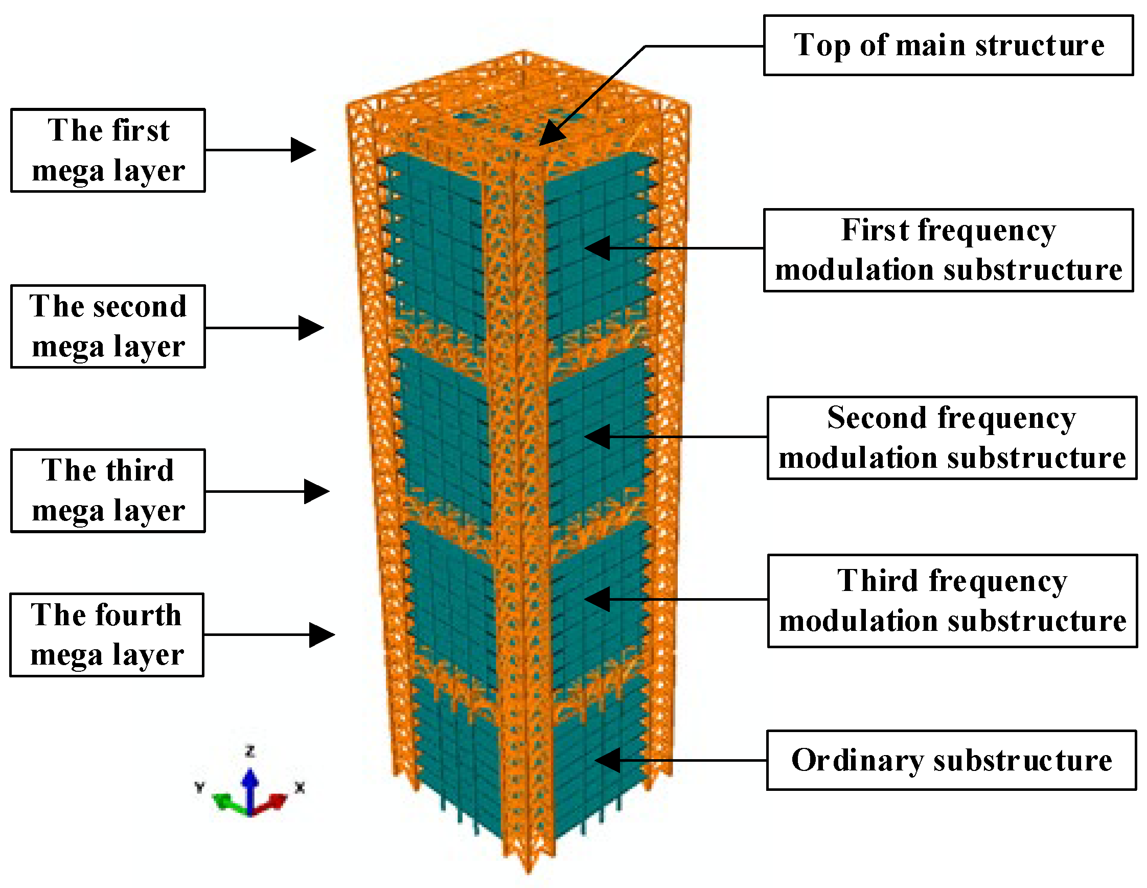
Analyzing the destruction patterns of the MSCSS under seismic forces is beneficial for strengthening the detailed design of an MSCSS. This paper aims to delve into the destruction patterns of the MSCSS under seismic forces, summarizing the damage situations to facilitate the establishment of reasonable damage configurations for MSCSSs. Based on this, achieving high-performance identification of damage types in this structure becomes a meaningful research endeavor.

2.1. MSCSS Modeling

Mega-sub controlled structural systems are divided into the main structure and substructure. The main structure consists of giant beams and giant columns, while the substructure serves as functional units for normal use. The entire structural system achieves damping through the tuning function of the substructure and the damping effect of dampers to achieve seismic mitigation, as illustrated in Figure 1.

The research subject of this paper, the MSCSS, has a total of 36 floors with a structure height of 144 m. The seismic design category of the structure is Class B, and the seismic fortification intensity in the region is grade VIII at 0.2 g. The constant floor load is 6.0 kN/m² (including the self-weight of the floor), and the live floor load is 2.0 kN/m². The strength grade of the steel used is Q345. For other modeling details of the MSCSS, please refer to references [22,23]. The section dimensions and parameters of each component on different floors are shown in

Table 1. The sectional characteristics of components in the mega-sub controlled structural model.

Component	Section Codes	Section Dimensions (mm)	Area (m2)	Ix (m4)	Iy (m4)
Giant columns	MC1-2 MC3-4	☐ 800 × 800 × 34 × 34 ☐ 600 × 600 × 20 × 20	0.1042 0.0464	0.0102 2.61 × 10−3	0.0102 2.61 × 10−3
Giant beams	MB1 MB2-4	H 588 × 300 × 12 × 20 H 582 × 300 × 12 × 17	0.0186 0.0168	1.133 × 10−3 9.79 × 10−4	9.008 × 10−5 7.66 × 10−5
Giant layer beam braces	MBBr1-3 MBBr4	☐ 350 × 350 × 20 × 20 ☐ 300 × 300 × 16 × 16	0.0264 0.0182	4.809 × 10−4 2.451 × 10−4	4.809 × 10−4 2.451 × 10−4
Giant layer column support	MCBr	☐ 250 × 250 × 14 × 14	0.0132	1.231 × 10−4	1.231 × 10−4
Beams in giant columns	MCB1-2 MCB3-4	H 582 × 300 × 12 × 17 H 500 × 250 × 10 × 18	0.0168 0.0137	9.79 × 10−4 6.101 × 10−4	7.66 × 10−5 4.730 × 10−5
Substructure beam	SC1-2 SC3-4	☐ 800 × 800 × 28 × 28 ☐ 600 × 600 × 20 × 20	0.0865 0.0464	8.600 × 10−3 2.61 × 10−3	8.600 × 10−3 2.61 × 10−3
Substructure column	SB	H 500 × 250 × 10 × 18	0.0136	6.06 × 10−4	4.69 × 10−5

. In the table, MC1-2 refers to the giant columns in giant layers 1 and 2, and MC3-4 represents the giant columns in giant layers 3 and 4. M is an abbreviation for a mega layer, C is an abbreviation for a column, B is an abbreviation for a beam, and Br is an abbreviation for a brace.

The MSCSS used in the study consists of three tuned substructures and one regular substructure. For the convenience of later discussion, the giant layers and substructures within MSCSS have been named, following the naming convention depicted in Figure 2.

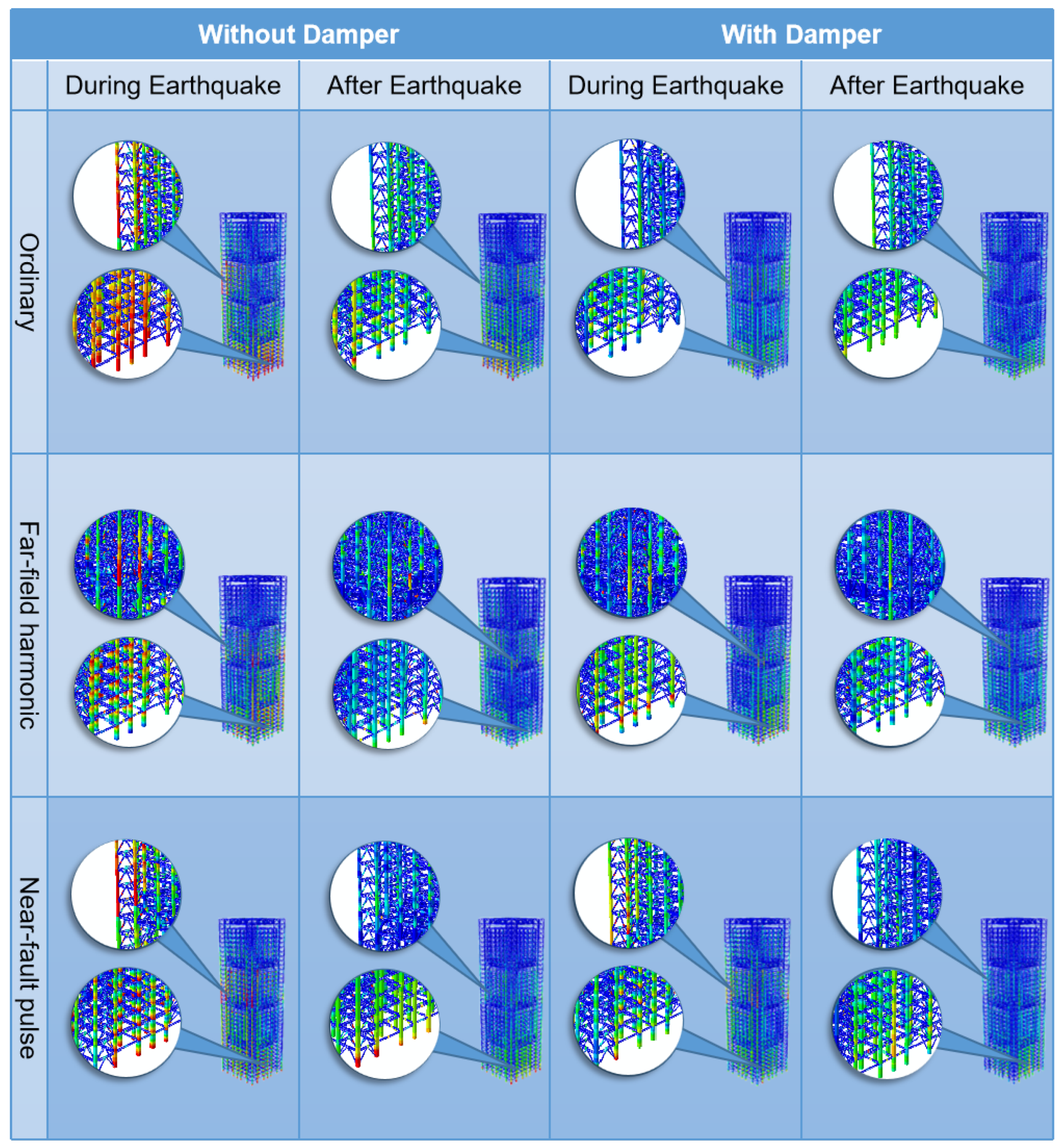
2.2. Damage Mechanism Study of MSCSS

To explore the influence of different types of seismic records on the damage mechanisms of the MSCSS, this study considers the effects of far-field harmonic and near-fault pulse long-period seismic records. Stress contour maps under the action of three typical seismic records on the MSCSS were extracted, as shown in Figure 3.

The following can be observed from Figure 3: (i) Compared with the stress contour maps of the two structures under the action of ordinary seismic records, the stress contour map of the second giant layer under the influence of near-fault pulse seismic records is significantly increased for both structures. (ii) Compared with the stress contour map of the structure under far-field harmonic seismic records, the stress contour map under the action of near-fault pulse seismic records is generally smaller. The damage in the second giant layer of the MSCSS without dampers is less than that under the far-field harmonic seismic records. (iii) After an earthquake, both structures exhibit residual stresses, and the residual stress in the MSCSS with dampers is significantly smaller than that in the MSCSS without dampers, indicating that the MSCSS with dampers is a more performance-optimized form. (iv) Under the action of near-fault pulse seismic records, the position where the fourth giant layer of the MSCSS without dampers connects to the foundation shows obvious yielding and significant damage, requiring extra attention in design. (v) Under the action of near-fault pulse seismic records, both structures experience stress in the first giant layer at the moment of maximum seismic amplitude. The main reason is that the near-fault pulse seismic records cause an increase in the acceleration response at the top of the structure. (vi) Under the action of three types of seismic records, the stress concentrations in both the MSCSS with dampers and the MSCSS without dampers are in the second main structure layer and the fourth main structure layer, indicating that the second giant layer and the fourth giant layer in both structures are more susceptible to damage.

2.3. Damage Modes Setting for MSCSS

Based on the actual seismic damage analysis results in Section 2.2, damage configurations were applied to the MSCSS, as shown in

Table 2. Damage mode configurations for MSCSS.

Damage Mode Code	Damage State Descriptions
MSCSS-F1	Undamaged State
MSCSS-F2	Setting 30% damage to all components in the second giant layer
MSCSS-F3	Setting 50% damage to all components in the second giant layer
MSCSS-F4	Setting 30% damage to all components in the fourth giant layer
MSCSS-F5	Setting 50% damage to all components in the fourth giant layer

. Different levels of damage were set for vulnerable locations, and the undamaged state of the structure was encoded as MSCSS-F1. Four different types of structural damage, varying in location and severity, were configured for the MSCSS. In this study, damage was implemented by reducing the elastic modulus of the steel. For example, a damage level of 30% indicates a 30% reduction in the elastic modulus of the structural components. MSCSS-F1 represents the undamaged state, while MSCSS-F2 to MSCSS-F5 represent the structure experiencing varying degrees of damage.

2.4. Damage Signal Acquisition and Dataset Preparation for MSCSS

In order to obtain synthetic seismic records with similar statistical characteristics, a method based on the Hilbert–Huang Transform (HHT) was employed for generating artificial seismic records. Specifically, the target power spectral density was set to match the progressive power spectrum of real seismic records. The artificial seismic records with the same power spectrum as real seismic records were then generated using Equation (1).

$${\ddot{x}}_{\mathrm{g}}={\displaystyle \sum _{k=1}^N\sqrt{4S\left(t,{\omega }_k\right)∆\omega }}\cos \left({\omega }_{k}t+{\varphi }_k\right),$$

(1)

where ${\ddot{x}}_{\mathrm{g}}$ represents the generated seismic record, $S\left(t,{\omega }_k\right)$ is the progressive power spectrum of seismic records, $∆\omega ={\omega }_k-{\omega }_{k-1}$ denotes the frequency interval, and ${\omega }_k$ is the instantaneous frequency of seismic records distributed randomly between 0 and 2π.

The progressive power spectrum of seismic records can be obtained by using the HHT, which primarily involves empirical mode decomposition (EMD) and Hilbert spectral analysis. For detailed theoretical aspects, please refer to [23]. The process of generating artificial seismic records is illustrated in Figure 4.

By generating artificial seismic records, the sample size has been expanded, ensuring that the samples share similar statistical characteristics. Time-history analysis was conducted on the MSCSS, resulting in structural response data for five different damage scenarios. Figure 5 illustrates the response of the first giant layer, the second giant layer, and the third giant layer under various damage states.

From Figure 5, it can be observed that the response of the MSCSS varies intuitively under different degrees of damage. The acceleration response of the first main structure layer is more pronounced under different damage levels, but other layers also contain effective damage signals within the structure.

3. Relevant Theories and the Proposed Damage Recognition Method

In this paper, a damage recognition method is designed by combining a one-dimensional convolutional neural network, ensemble heterogeneous learning classifiers, and a meta-learner. Here, we will elaborate on the introduction of the related theories, methodology, and the preparation of experimental data, and the process of training the model.

3.1. Related Theories

Convolutional neural networks (CNNs), as a classic neural network model, have achieved success not only in traditional fields such as computer vision and natural language processing but also in various applications [35,36]. They are primarily composed of convolutional layers, pooling layers, and fully connected layers.

A CNN is typically designed to process two-dimensional images, and this type of network is referred to as a 2DCNN. However, to leverage CNNs for extracting features from one-dimensional signals, a corresponding 1DCNN structure is necessary. The basic structure of a one-dimensional convolutional neural network is similar to that of a 2DCNN, consisting of convolutional layers, pooling layers, and fully connected layers. The convolutional layer is responsible for extracting local features, the pooling layer reduces feature dimensions, and the fully connected layer is utilized for classification or regression tasks.

The 1D convolutional layer consists of a set of learnable convolutional kernels, where each kernel slides over the input data, computing a linear weighted sum for the local region. The output of each convolutional kernel is referred to as a feature map, which reflects local patterns in the input data. The 1D pooling layer is used to reduce the dimensionality of the feature maps, decreasing the number of network parameters and computational load. Common pooling operations include max pooling and average pooling. Max pooling extracts the most prominent features from the feature maps, while average pooling calculates the average value of the feature maps.

Stacking ensemble theory. Given the difficulty in selecting the best-performing model from different classification models, as each classifier has its own strengths and there may not be a unique optimal classifier, combining the results of different classifiers to make the final classification decision is a solution known as ensemble learning. This paper utilizes the Stacking ensemble method for high-precision classification of structural damage recognition features. The Stacking ensemble method merges the results of different machine learning classifier models to obtain more accurate and stable classification results [37,38]. The basic idea of this ensemble method is to first use multiple models to classify the input data features, integrate the classification results of multiple models, and obtain the final classification result. These models are referred to as base models, and the specific integration method involves using the predictions of multiple models as new features to train another model, known as the meta-learning model.

There are two stages of models in the stacking method. The models in the first stage take the original training set as input and are called base models or base learners (also known as level-one learners), and various base models can be selected for training. The models in the second stage take the predictions of the base models on the original training set as the training set and the predictions of the base models on the original testing set as the testing set. These models are called meta-models (also known as level-two learners). The stacking ensemble learning framework is shown in Figure 6.

In the Stacking method, primary learners are trained from the initial dataset, and then a new dataset is ‘generated’ for training secondary learners. In this new dataset, the output of primary learners serves as the input feature, while the labels of the initial samples are still treated as example labels. It is worth noting that the Stacking ensemble method requires training both base models and meta-learners during the training phase. When training base models, each base model uses the entire training set for training, employing a cross-validation strategy during training. Then, the Stacking method trains a meta-learning classifier model to combine the outputs of the previously trained base models. The specific process involves constructing the outputs of previously trained base models into a training set and using it as input to train a model to obtain the final output.

Base learners. The selection of four base learners is designed to achieve complementary feature extraction through heterogeneous algorithmic mechanisms: Gradient Boosting Decision Tree (GBDT) and Random Forest (RF) are employed to generate class probability estimates that encode model confidence information, while k-Nearest Neighbors (KNN) provides discrete voting outcomes derived from local neighborhood patterns. Support Vector Regression (SVR) contributes continuous decision values through its kernel-based optimization framework. This strategic integration of distinct prediction paradigms enables the synthesis of a multi-dimensional meta-feature space that comprehensively preserves both global discriminative patterns and localized data characteristics.

Gradient Boosting Decision Tree (GBDT) utilizes the residuals of the previous tree as the fitting target for the next tree, continuously accumulating the results of multiple base classifiers to ultimately obtain a powerful classification model [39]. The fundamental principle of GBDT is to iteratively approximate the true function by fitting the residuals. Assuming the true function is F(x), it is approximated through a linear combination of a set of base functions h(x), and this can be calculated using Equation (2):

$$F(x)\approx {\displaystyle \sum _{m=1}^M{h}_m}(x),$$

(2)

herein, h_m(x) represents a decision tree. In the m-th round of iteration, what needs to be fitted are the residuals generated by the current model:

$$r_{im}=-[{\displaystyle \frac{𝜕L(y_i,F(x_i))}{𝜕F(x_i)}}]F(x)=F_{m-1}(x_i),$$

(3)

where $L(y_i,F(x_i))$ is the loss function, y_i is the true label value of the sample x_i, and $F_{m-1}(x_i)$ is the prediction obtained from the first m-1 rounds of iteration.

Using a new tree to fit the residual r_im is carried out to reduce the residual value. A piecewise function p_m(x) is introduced into the new tree, updating the prediction of the current model to be:

$$F_m(x)=F_{m-1}(x)+p_m(x),$$

(4)

As is evident, the new tree needs to fit the residual r_im, and this process is an iterative one of continuously fitting residuals.

Random Forest (RF) is an ensemble model consisting of multiple decision trees, and it is a well-performing classifier. When used for classification, the training process of each decision tree employs the Gini coefficient to determine the splitting feature [40]. The magnitude of the Gini coefficient can be used to describe whether the classification is correct and can be calculated according to Equation (5).

$$Gini(p)={\displaystyle \sum _{k=1}^k{P}_k}(1-P_k)=1-{\displaystyle \sum _{k=1}^k{P}_k^2},$$

(5)

where $P_k$ represents the probability of a sample belonging to class k, and $(1-P_k)$ denotes the probability of a sample not belonging to class k.

The final classification result of the RF algorithm is determined by a majority vote based on the classification results of each decision tree. The classification process can be represented using Equation (6).

$$H(x)=\arg \max {\displaystyle \sum _{i=1}^{K}I}\left(h_i(x)=\mathrm{Y}\right),$$

(6)

where H(x) is the final classification result, h_i(x) represents the classification result of an individual decision tree, and Y denotes the category label for structural damage.

The principle of k-Nearest Neighbors (KNN), in simple terms, is to determine the category of a sample based on the categories of the nearest samples [41]. For an unknown sample, KNN identifies the k nearest training samples and then determines the category of the unknown sample by voting or averaging the labels of these k training samples. KNN involves comparing the feature distances from a given sample to other samples, with commonly used distance metrics such as Manhattan distance, Euclidean distance, cosine similarity, etc. Manhattan distance, for example, represents the sum of absolute axis distances between two points in a standard coordinate system. For a two-dimensional space, the calculation formula for the Manhattan distance is:

$$d\left(x,y\right)=\left|{{\displaystyle x}}_1-{{\displaystyle y}}_1\right|+\left|{{\displaystyle x}}_2-{{\displaystyle y}}_2\right|,$$

(7)

In n-dimensional space, the formula for calculating the Manhattan distance is:

$$d\left(x,y\right)={\displaystyle \sum _{i=1}^n\left|{{\displaystyle x}}_i-{{\displaystyle y}}_i\right|},$$

(8)

Support Vector Regression (SVR) establishes a regression model by finding an optimal hyperplane in the training data to maximize the margin between predicted values and actual values while maintaining a certain tolerance range [42,43]. Specifically, assuming the training data can be represented by Equation (9), the hyperplane model can be expressed using Equation (10).

$$D=\{(X_1,Y_1),(X_2,Y_2),\cdots (X_n,Y_n)\},$$

(9)

$$f(x)=wx+b,$$

(10)

where X_i represents the input feature vector, Y_i is the corresponding output value, w is the normal vector, and b denotes the bias.

The optimization objective of SVR includes both the squared error term and the regularization term. In essence, its mathematical model can be simplified to the minimization problem as shown in Equation (11). This means that the distance between sample points and the hyperplane should not exceed the tolerance range.

$$\begin{array}{l}\underset{w,b,\xi ,{\xi }^{*}}{\min }{\displaystyle \frac{1}{2}}||w|{|}^2+C{\displaystyle \sum _{i=1}^n({\xi }_i+{\xi }_i^{*})}\\ subject to \left\{\begin{array}{l}{y}_i-w^T\varphi (x_i)-b\le ϵ+{\xi }_i^{*}\\ w^T\varphi (x_i)+b-y_i\le ϵ+{\xi }_i^{*}\\ {\xi }_i\ge 0, {\xi }_i^{*}\ge 0, i=1,2\cdots ,n\end{array}\right.\end{array},$$

(11)

where ${\xi }_i$ is the left slack variable, ${\xi }_i^{*}$ is the right slack variable, $y_i$ is the true target value for the i-th sample in the training set, $\varphi (x_i)$ is the corresponding feature vector, and C is the penalty coefficient.

Meta-learner. Referring to the aforementioned level-two learning model, the term “meta” here, as in meta-learning or meta-universe, conveys a higher level of abstraction. A meta-learner is essentially a “learner of learners” designed to learn from the outcomes of base learners. It can be understood as a weighted average and scorer for the base learners [44]. This paper selects the sparse SVM classifier as the meta-learner. Its basic theory is as follows:

Sparse Support Vector Machine (sparse SVM) is a variant of SVM designed to address classification problems on high-dimensional sparse datasets [45]. Compared to traditional SVM, sparse SVM maintains model performance while automatically selecting fewer support vectors, thereby enhancing model fitting speed and generalization ability.

A commonly used implementation of sparse SVM involves utilizing L1 regularization to encourage the model to select sparse features. L1 regularization achieves this by adding an L1 norm penalty when minimizing the objective function. This approach leads to some feature weights becoming zero, thereby achieving feature sparsity.

The specific algorithmic process of sparse SVM is outlined as follows:

(i)

Data preparation: Prepare the training dataset, including input features and their corresponding labels.

(ii)

Feature selection: Conduct feature selection on the input features, choosing a subset of important features as support vectors.

(iii)

Data standardization: Standardize the selected features, ensuring they exhibit zero mean and unit variance characteristics.

(iv)

Solving sparse SVM: Solve the optimization problem to obtain the parameters of the sparse SVM model. The objective function for sparse SVM can be expressed as:

$$\underset{w,b,\xi }{\min }{\displaystyle \frac{1}{2}}{‖w‖}^2+C{\displaystyle \sum }_{i=1}^n{\xi }_i,$$

(12)

where $w$ is the model’s weight vector, $b$ is the model’s bias term, $\xi$ is the slack variable, and C is the regularization parameter.

The objective function of sparse SVM, compared to traditional SVM, includes an additional sparsity penalty term, used to control the selection of support vectors. The objective of sparse SVM is to minimize the objective function, finding suitable values for $w$ and $b$, and adjusting the slack variables to control misclassified samples.

(v)

Model prediction: Utilize the obtained sparse SVM model to predict new samples. The prediction formula is:

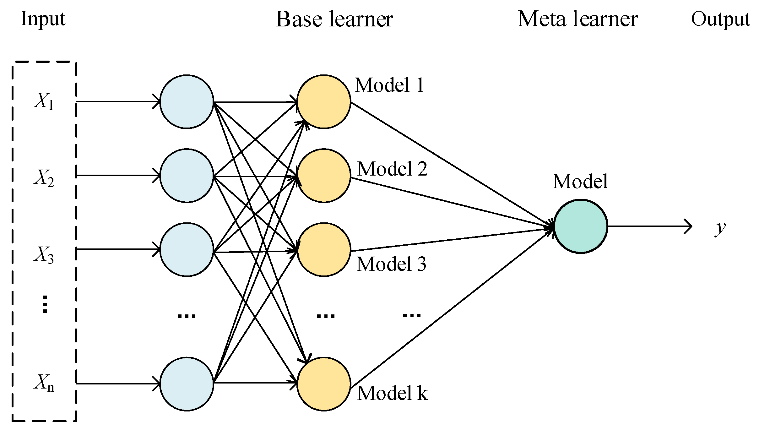
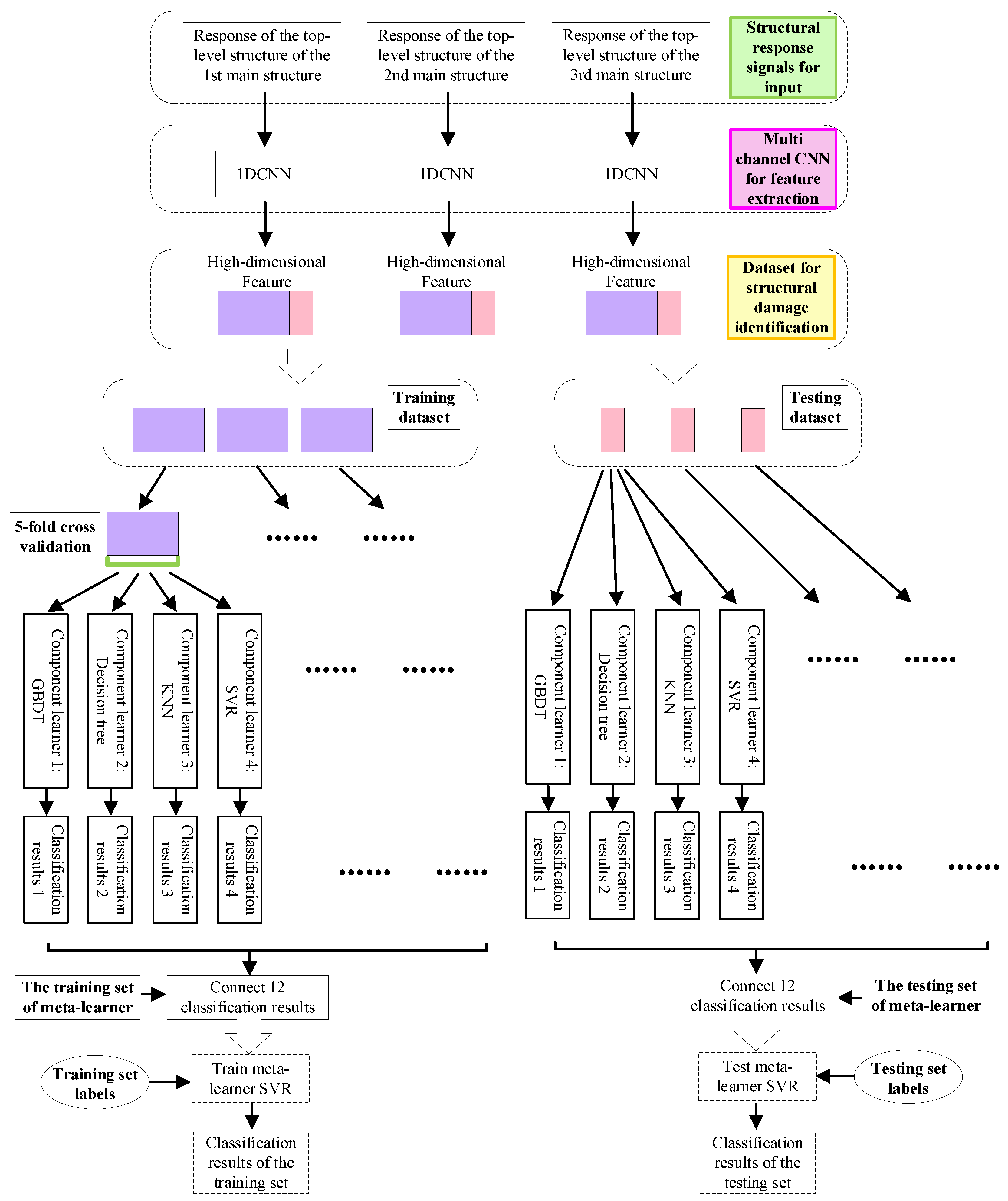
$$y=sign(w^{T}x+b),$$

(13)

where x is the feature vector of the sample to be predicted, and y is the predicted class of the sample.

3.2. Methodology

In order to address the issue of significant dependence on the choice of identification signal types in existing structural damage recognition methods, this paper proposes a structural damage recognition method based on the combination of multi-channel feature exploration and integrated heterogeneous classification learning. The framework of the proposed method is illustrated in Figure 7.

Specifically, the proposed method combines a three-channel CNN and a stacking ensemble heterogeneous learning model. Considering that the MSCSS structure designed in this article contains three frequency modulation substructures, the acceleration response signal of the top-level structure of the three main substructures of the MSCSS is used as the information source for damage identification. It should be pointed out that if the identified structure has more representative structural response signals, the input signals can be determined according to the specific situation, and then the damage recognition model can be trained. The stacking ensemble heterogeneous learning model includes four base classifiers (GBDT, Random Forest, KNN, SVR) and one meta-learner (sparse SVM meta-learner). Therefore, the proposed method is referred to as 3C-EHSML, where “3C” represents three-channel CNN, “EH” refers to ensemble heterogeneous, and “SML” indicates sparse SVM meta-learner. By analyzing the acceleration response signals of the top-level structures of the three main structures of the MSCSS, the method utilizes three 1DCNNs to extract high-dimensional feature information from acceleration response signals. Then, based on the stacking ensemble heterogeneous learning model, it classifies the high-dimensional features for fault diagnosis. The proposed stacking ensemble heterogeneous learning model includes four classifiers, also known as weak learners, to avoid large errors from a single weak learner. By combining multiple weak learners, the classification results are concatenated and input to the meta-learner. The training set’s weak learner learning results are used as input, and the output of the training dataset is used as output to train a meta-learner to obtain the final result.

The main parameter settings in the proposed damage identification model are shown in

Table 3. Parameter selection of machine learning model.

GBDT		RF		SVR		KNN
n_estimators	200	n_estimators	230	C	10	n_neighbors	12
learning_rate	0.15	max_depth	20	epsilon	0.6	weights	uniform
max_depth	6	min_samples_split	30	kernel	sigmoid	algorithm	auto
min_samples_split	30	min_samples_leaf	25	gamma	auto	leaf_size	25
min_samples_leaf	20	max_features	0.3

.

3.3. Experimental Dataset Setting and Training of Damage Recognition Model

The acceleration response signals from the top-level structures of the first, second, and third main structures were separately collected in this study. By introducing noise into the structures, 500 samples were collected for each signal type. The training and testing dataset split ratio is 4:1. During the training process, the training set is further divided into training data and validation data in a 4:1 ratio.

The training phase mainly involves the following steps:

(i)

Dividing the training samples into k-fold cross-validation samples and performing 5-fold cross-validation experiments for all four base learners, creating training samples for the base learners.

(ii)

Training the four base learners on the cross-validation samples, obtaining the prediction results for each base learner, and saving them.

(iii)

Concatenating the prediction results of the 12 base learners from the three 1DCNN models and inputting them into the meta-learner.

(iv)

The meta-learner takes the concatenated results of the base learners’ outputs as training samples, with the training set labels marked as structural damage types.

(v)

Comparing the predictions of the meta-learner with those of the base learners to assess whether the model’s performance after employing the stacking ensemble strategy is superior to that of individual models.

The prediction phase of the structural damage recognition model mainly includes the following steps:

(i)

Inputting the test samples into the trained base learners to obtain the prediction results for each base learner.

(ii)

Concatenating the prediction results of the base learners from the multi-channel 1DCNN model and inputting them into the meta-learner. The input samples for the meta-learner testing are the concatenated results, and the labels of the test samples are marked as structural damage types.

(iii)

Comparing the predictions of the meta-learner with those of the base learners to test whether the performance of the model after using the stacking ensemble strategy is better than that of a single model.

4. Results and Discussion

4.1. Evaluation Indexes

The effectiveness of the structural damage recognition model needs to be measured using metrics. This paper employs four comprehensive indices, namely Accuracy (A), Precision (P), Recall (R), and F1-score (F1), to evaluate the results. These four indices can be calculated using Equations (14)–(17).

$$A={\displaystyle \frac{TP+TN}{TP+FN+FP+TN}},$$

(14)

$$Precision={\displaystyle \frac{TP}{TP+FP}},$$

(15)

$$Recall={\displaystyle \frac{TP}{TP+FN}},$$

(16)

$$F_1-Score=2\cdot {\displaystyle \frac{Precision\cdot Recall}{Precision+Recall}},$$

(17)

where TP (True Positive) refers to the number of samples predicted as positive and actually being positive, FP (False Positive) refers to the number of samples predicted as positive but actually being negative, FN (False Negative) refers to the number of samples predicted as negative but actually being positive, and TN (True Negative) refers to the number of samples predicted as negative and actually being negative.

4.2. The Results of Structural Damage Detection

The provided method was employed for 10 experiments on the damage signals of the MSCSS, with the results documented in

Table 4. The results of conducting structural damage detection using the proposed method for 10 trials.

Trial Number	1	2	3	4	5	6	7	8	9	10
Accuracy (%)	98.6	98.0	98.2	99.2	98.0	99.6	1.00	98.6	99.4	99.8
Acc_ave + Var	98.9% ± 0.21

. Detailed outcomes of one of the experiments are recorded in

Table 5. The specific results of structural damage detection for one trial using the provided method.

	F1	F2	F3	F4	F5	Precision	Recall	F1-Score
F1	100					0.9901	1	0.9950
F2	1	98	1			0.9899	0.98	0.9849
F3		1	96	3		0.96	0.96	0.96
F4			3	97		0.97	0.97	0.97
F5					100	1	1	1

.

From Table 4 and Table 5, it can be observed that the average accuracy of the proposed damage detection method exceeds 98%. The misclassification of damage is primarily concentrated between F2 and F3, as well as between F3 and F4. As indicated in Table 2, three F3 samples were misclassified as F4, and three F4 samples were misclassified as F3. Additionally, the damage modes of F1 and F5 were correctly identified.

In order to verify the advantages of using three channel signals for damage identification, damage identification experiments were conducted using only two channels and one channel. The average accuracy of 10 experimental results is shown in

Table 6. Damage identification results under different numbers of channels.

Channel Settings	1	2	3	1 + 2	1 + 3	2 + 3
Accuracy (%)	94.5	94.3	93.9	96.8	96.5	96.3

, where “1–3” represents the 1–3 frequency modulation substructures of the MSCSS.

According to Table 6, the overall performance of using two channels is better than using one channel, and the performance of using three channels is still the best.

4.3. The Setting of Comparison Methods

To demonstrate the advantages of the proposed structural damage detection method based on the integration of multi-channel feature extraction and stacking ensemble heterogeneous classification learning, three categories and a total of seven comparison methods were set up from the perspectives of signal feature extraction, feature pre-classification, and decision classification included in the proposed method. The first category distinguishes itself from the proposed method by using a multi-channel CNN to explore structural response signal features. Comparison method 1 extracts 24 time–frequency domain features of the structural response signal for subsequent damage category classification. This method is abbreviated as TF-EHSML. The second category involves setting up comparisons with the stacking ensemble heterogeneous classification base model used in the proposed method. There are three comparison methods in this category. Comparison method 2 designs a stacking ensemble homogeneous base model, where all four base models are Random Forests. This method is abbreviated as 3C-ERSML. Comparison method 3 has all four base models as KNN, abbreviated as 3C-EKSML. Comparison method 4 integrates heterogeneous base models with three designed base models: GBDT, Random Forest, and KNN. This method is abbreviated as 3C-E3HSML. The third category of comparison methods involves comparing from the perspective of meta-learners. Methods based on naive Bayes, Random Forest, and Logistic Regression are compared as comparison methods 5 (3C-EHNML), 6 (3C-EHRML), and 7 (3C-EHLML), respectively. It is worth noting that the design of these three categories of comparison methods is based on the principle of the controlled variable method. Each comparison method differs only in one component from the proposed method, while the remaining two parts remain unchanged.

4.4. Performance Comparison of Different Recognition Methods

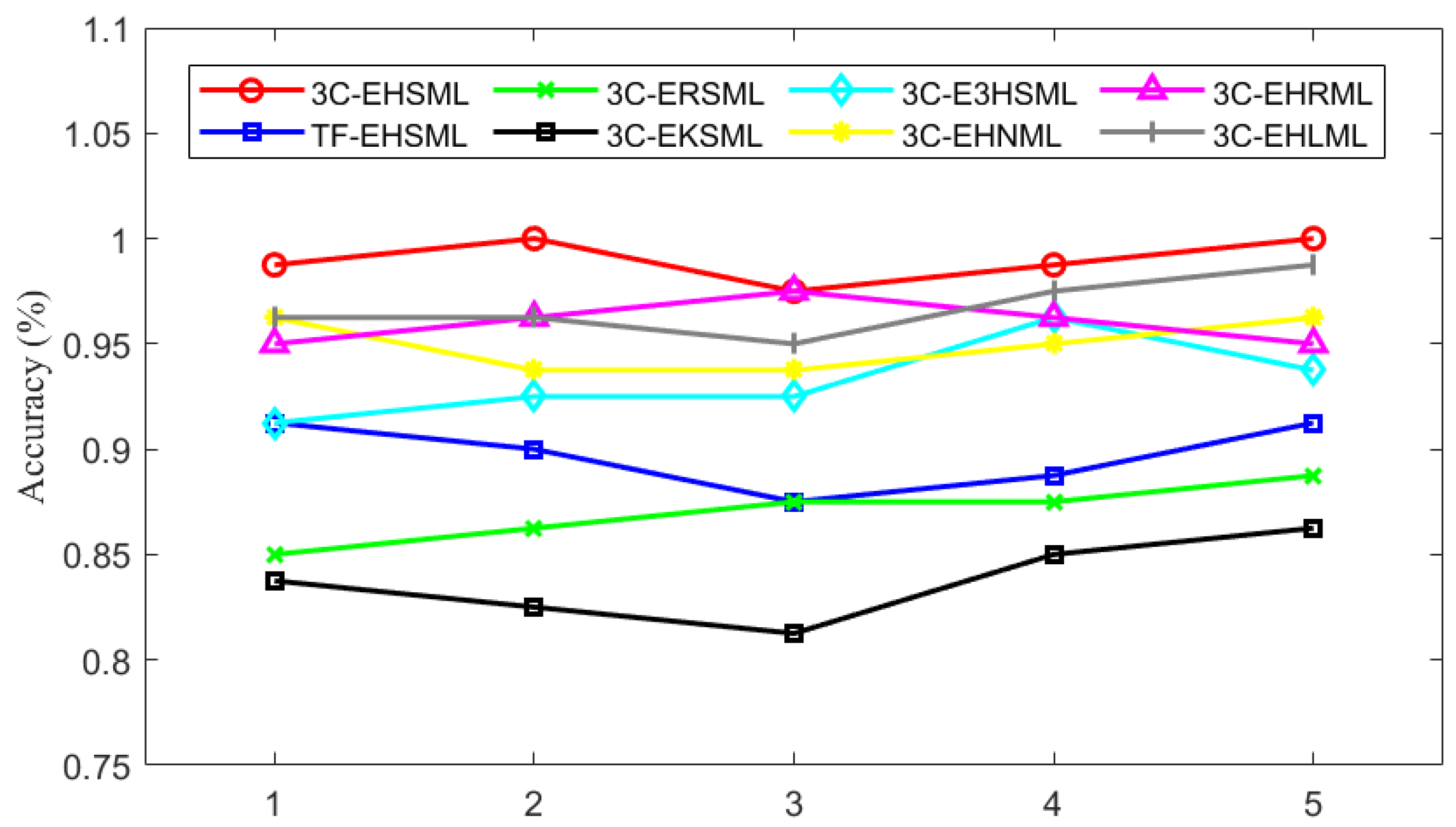
4.4.1. Comparison of Model Training Performance

During the model training phase, a five-fold cross-validation was employed to enhance the generalization capability of structural damage detection. By repeatedly partitioning the training set and validation set and calculating the model training error, the training process of the model becomes more comprehensive. For the proposed method 3C-EHSML and the seven comparison methods, the recognition accuracy on the validation set within the training set during five-fold cross-validation is illustrated in Figure 8.

Based on Figure 8, overall, the proposed method 3C-EHSML consistently exhibits the highest accuracy in the five-fold cross-validation, with accuracy consistently exceeding 97% across all five training stages. In contrast, the accuracy of the comparison methods is generally lower than that of the proposed method, and the third comparison method, 3C-EKSML, demonstrates the poorest recognition performance with an average accuracy of approximately 83%. This indicates a significant advantage of stacking ensemble heterogeneous base models over ensemble homogeneous base models. Furthermore, as the performance of comparison method 3 is slightly weaker than that of comparison method 2, it suggests that in the context of structural damage detection in MSCSS, the performance of the Random Forest classifier is slightly stronger than that of KNN. Overall, among the comparison methods, the third category of methods (meta-learners) exhibits the best damage recognition performance, with specific rankings being comparison method 7 (3C-EHLML), followed by comparison method 6 (3C-EHRML), and lastly, comparison method 5 (3C-EHNML). This indicates that the choice of meta-learner has a relatively small impact on the performance of structural damage detection. Additionally, following the well-performing methods, comparison method 4 (3C-E3HSML) achieves an average accuracy of approximately 93%, demonstrating that stacking heterogeneous base models has a greater advantage in classification compared to homogeneous base models. Comparison method 1 (TF-EHSML) has an average accuracy of around 90%, weaker than the meta-learner series but stronger than methods with homogeneous base models. This suggests that time-frequency domain features can, to some extent, reflect differences between signals of different structural damage types. However, the representational power of these features is weaker than the automatically extracted features by the multi-channel CNN. In summary, among the three categories of comparison methods, the methods with stronger performance are comparison method 1 (TF-EHSML), comparison method 4 (3C-E3HSML), and comparison method 7 (3C-EHLML).

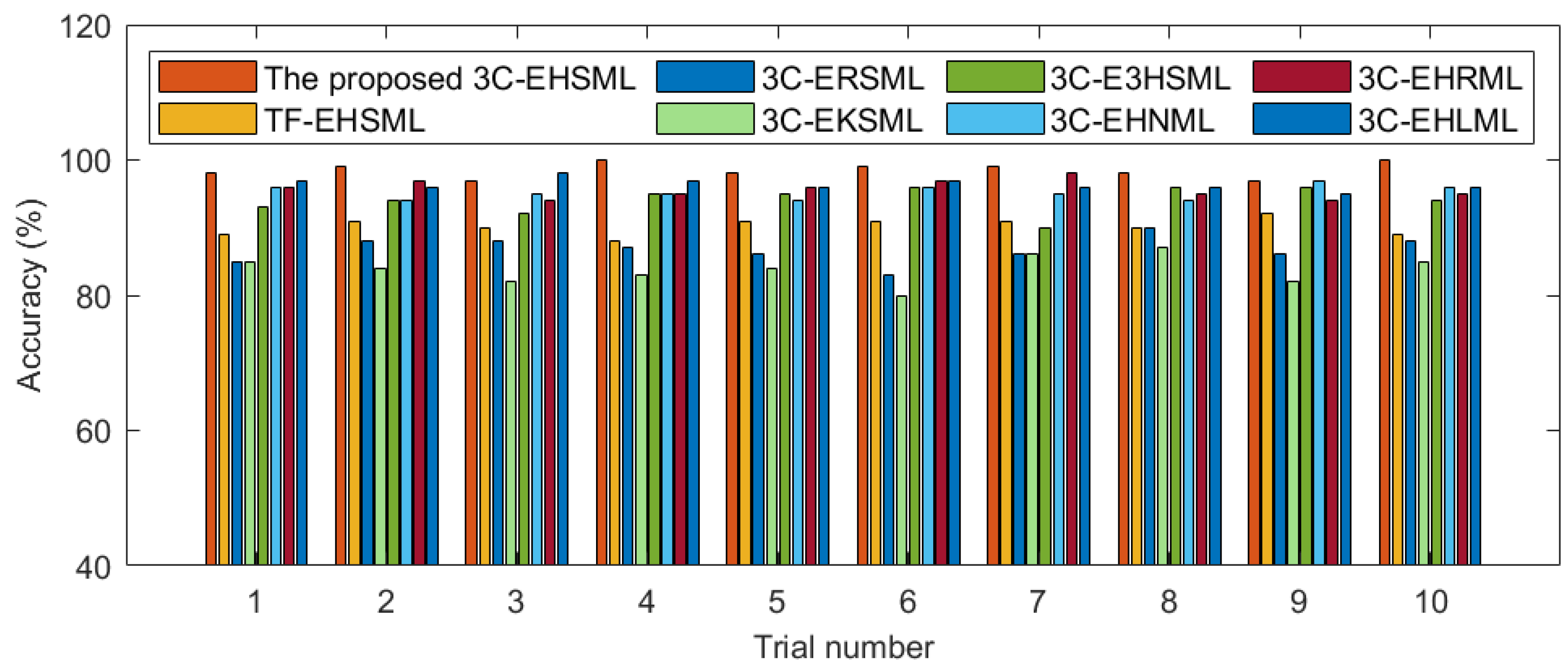
4.4.2. Different Models’ Test Performance Comparison

After completing the model training, testing was conducted on the testing dataset. In the testing dataset, there were 100 samples for each damage mode, making a total of 500 test samples across five damage modes. The proposed method and the seven comparison methods were each tested in 10 experiments. As shown in Figure 9, the damage recognition accuracy for each method is displayed for the 10 test trials.

From Figure 9, it is evident that the recognition performance of the proposed method consistently surpasses all comparison algorithms over the 10 test trials, consistently staying above 97%. However, its accuracy is relatively close to comparison methods 5 (3C-EHNML), 6 (3C-EHRML), and 7 (3C-EHLML). Unlike Figure 9, which shows the accuracy of various damage recognition methods over 10 test trials, Figure 10 provides a box plot comparing the 10 test trials of the proposed method with the comparison methods from a methodological perspective, illustrating the distribution of recognition performance for each method.

From Figure 10, it is evident that the accuracy of the proposed structural damage recognition method is the highest. From the perspective of the height of the 25–75% range, the distribution of accuracy for the proposed method is the most concentrated, while the distribution for comparison method 3 is the most scattered. The mean accuracy of the proposed method is generally distributed in the middle of the 25–75% range.

Furthermore, to visually demonstrate the superiority of the proposed damage recognition method, the performance of the corresponding models was tested after model training. The recognition results for the proposed method and the three worst-performing methods among the various comparison methods are provided here, specifically illustrated in the form of a confusion matrix plot (as shown in Figure 11).

In Figure 11, the horizontal axis of the confusion matrix represents predicted labels, while the vertical axis represents true labels. Along the diagonal, which indicates correct classifications, values closer to 100 indicate better recognition performance for structural damage types. As seen in Figure 11, the proposed method has minimal misclassifications and exhibits the best recognition performance compared to the remaining three comparison methods. All three comparison methods show varying degrees of misclassifications, with the most frequent misclassifications occurring between F3 and F4, followed by F1, F2, and F3. The misclassification rate for F5 is relatively lower compared to the other four damage modes.

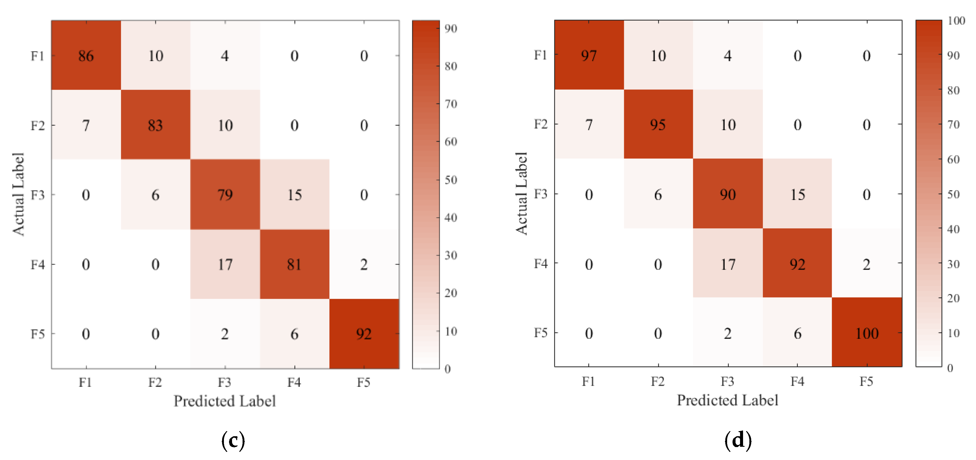
4.4.3. The Comparison Experiment for Imbalanced Data

In practical engineering scenarios, structural damage states are less frequent compared to the normal state. Therefore, in real-world applications, the number of actual structural damage signals (F2–F4) is less than the number of normal state signals (F1). To analyze the performance of the proposed structural damage recognition algorithm under imbalanced conditions, this study designed five imbalanced scenarios as shown in

Table 7. Details of five imbalanced dataset cases.

Imbalanced Case	Imbalanced Ratio	The Number of Samples for Normal State			The Number of Samples for Each Damage State
		Training Dataset	Validation Dataset	Testing Dataset	Testing Dataset	Validation Dataset	Testing Dataset
Case 1	1:1	320	80	100	320	80	100
Case 2	1:0.9	320	80	100	288	72	100
Case 3	1:0.8	320	80	100	256	64	100
Case 4	1:0.7	320	80	100	224	56	100
Case 5	1:0.6	320	80	100	192	48	100

.

As shown in Table 7, the differences in sample quantities are reflected during the training phase in the five imbalanced cases. For the testing dataset, the sample quantities for each damage mode in various imbalanced states and the balanced state are all set to 100. In the case of a balanced dataset, corresponding to case 1 in Table 1, the training dataset and validation dataset have a ratio of 4:1, with sample quantities of 320 and 80, respectively. In the remaining four imbalanced cases, the ratio of the training dataset to the validation dataset remains 4:1. However, the sample quantities for each damage mode in the training dataset and validation dataset decrease proportionally compared to the normal state. For example, in the case of an imbalance ratio of 1:0.9, the sample quantity for each damage state in the training set is 320 * 0.9, which equals 288. Subsequently, the performance of various damage recognition methods will be compared and analyzed under the five imbalance ratios.

The proposed method and seven comparison methods were tested for performance in 10 experiments under each of the five imbalanced cases, and the results are presented in

Table 8. The performance of the proposed method and seven comparison methods in 10 experiments under different imbalanced cases.

Imbalanced Case	Case 1	Case 2	Case 3	Case 4	Case 5	The Degree of Decline
Proposed method	98.5 ± 1.05	95.2 ± 1.35	91.7 ± 1.46	87.2 ± 1.68	82.8 ± 1.89	15.7
TF-EHSML	90.2 ± 1.36	87.1 ± 1.58	82.8 ± 1.87	77.2 ± 2.04	71.8 ± 2.79	18.4
3C-ERSML	86.7 ± 3.41	82.0 ± 3.64	76.9 ± 3.93	70.3 ± 4.11	62.1 ± 4.51	24.6
3C-EKSML	83.8 ± 3.96	79.6 ± 4.27	76.1 ± 4.67	72.6 ± 5.12	66.5 ± 5.40	25.3
3C-E3HSML	94.1 ± 3.49	90.7 ± 3.73	85.3 ± 3.99	79.4 ± 4.54	70.9 ± 5.02	23.2
3C-EHNML	95.2 ± 0.96	91.8 ± 1.24	86.2 ± 1.67	80.1 ± 1.93	73.6 ± 2.26	21.6
3C-EHRML	95.7 ± 1.61	92.3 ± 1.93	87.0 ± 2.25	80.8 ± 2.67	74.4 ± 3.14	21.3
3C-EHLML	96.4 ± 0.64	94.7 ± 1.14	89.6 ± 1.54	84.3 ± 1.88	78.4 ± 2.13	18.3

.

It can be seen from Table 8 that the performance of the proposed method gradually decreases as the imbalance level deepens, i.e., as the imbalance ratio increases. From a balanced state to imbalanced case 5, the accuracy of structural damage recognition decreases by a total of 15.7%, and the variance also increases slightly. Among the comparison methods, comparison method 3 exhibits the largest decrease in accuracy, surpassing 25%. Comparison method 1 and comparison method 7 experience relatively smaller drops in accuracy, with decreases of 18.4% and 18.3%, respectively. In terms of accuracy, when the imbalance ratio is high, the proposed method has the highest accuracy, followed by comparison method 7, comparison method 6, comparison method 5, and comparison method 1.

To showcase the specific classification performance for different damage modes,

Table 9. The damage recognition performance of the proposed method in one experiment under balanced state and imbalanced case 3.

Index	Balanced State			Imbalanced Case 3
	Precision	Recall	F1-Score	Precision	Recall	F1-Score
F1	0.9901	1	0.9950	0.9588	0.93	0.9442
F2	0.9899	0.98	0.9849	0.92	0.92	0.92
F3	0.96	0.96	0.96	0.8365	0.87	0.8529
F4	0.97	0.97	0.97	0.8713	0.88	0.8756
F5	1	1	1	0.9898	0.97	0.9797

provides the damage recognition performance of the proposed method in one experiment under balanced state and imbalanced case 3. The table presents the effectiveness of structural damage recognition in terms of precision, recall, and F1-score metrics.

According to Table 9, it can be seen that the overall values of all three indices are higher in the balanced state compared to imbalanced case 3. For instance, in terms of precision, the precision for all five damage modes (F1–F5) is higher in the balanced state than in imbalanced case 3. Regarding the recall index, the proposed method achieves a recall of 1 for damage types F1 and F5 in the balanced state, indicating that all samples of these two damage types are correctly identified. However, the trends in structural damage recognition effectiveness across the five damage modes, as reflected by the three different indices, remain consistent between the two states.

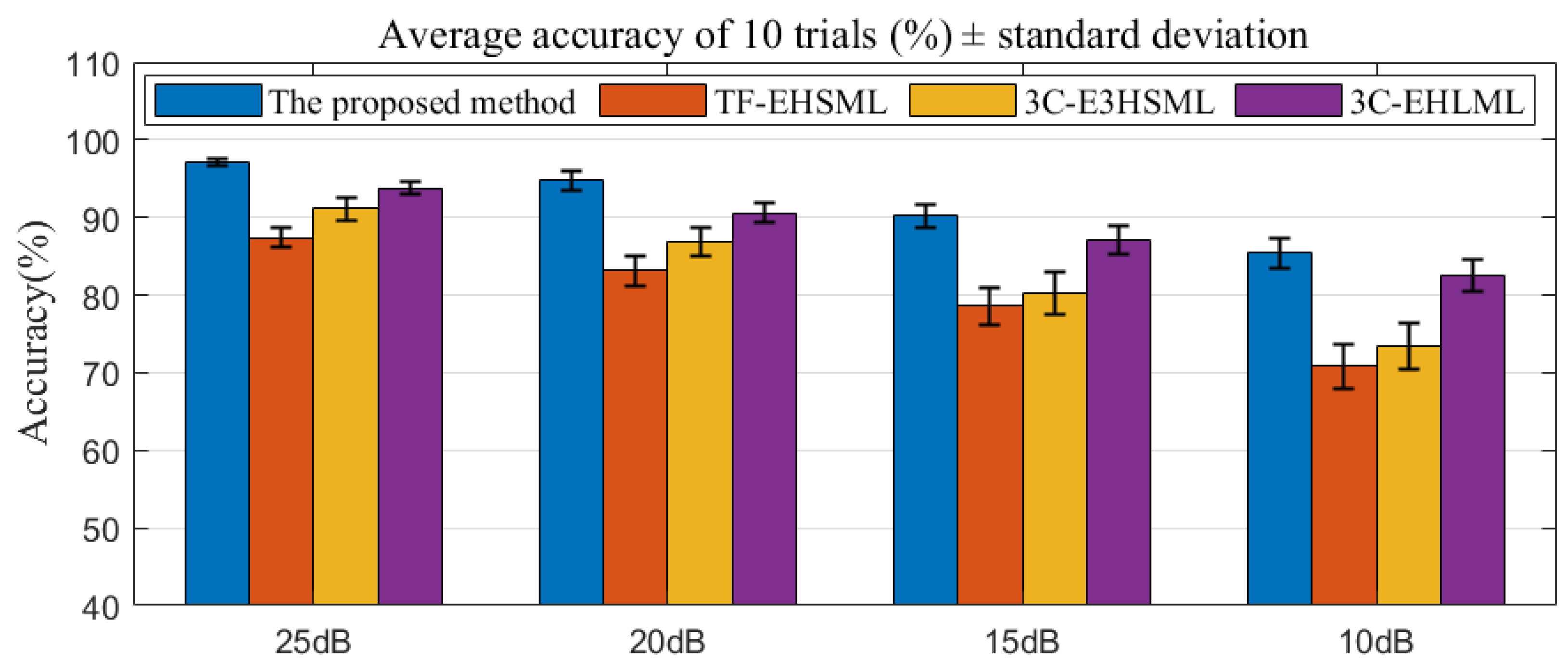
4.4.4. Noise Robustness Analysis

To explore the performance of the proposed method under the condition of noise in structural damage signals, based on the results in Section 4.4.2, the robustness to noise was tested for the proposed method and the remaining three comparison methods with good performance. These include comparison method 1 (TF-EHSML), comparison method 4 (3C-E3HSML), and comparison method 7 (3C-EHLML). Noise at different levels was added to the input signals, and the noise level was determined based on the signal-to-noise ratio (SNR) defined in Equation (18).

$$SNR(\mathrm{dB})=20\log {\displaystyle \frac{A_{signal}}{A_{noise}}}$$

(18)

where A_signal and A_noise represent the root mean square of the signal and noise, respectively. Four SNR levels were chosen: 25 dB, 20 dB, 15 dB, and 10 dB. Ten experiments were conducted for each of the proposed method and the three comparison methods. Figure 12 displays the average accuracy and variance of structural damage recognition for these methods across the 10 experiments.

As can be seen from Figure 12, it is evident that the performance of the proposed method and the three comparison methods declines as the SNR decreases from 25 dB to 10 dB. In terms of the extent of performance decline, the proposed method (11.7%) and comparison method 7 (11.3%) exhibit similar decreases, indicating that replacing the meta-learner has a minimal impact on the noise resistance of the damage recognition method. Conversely, comparison methods 1 and 3 experience larger decreases in accuracy, with reductions of 16.6% and 17.7%, respectively, as the noise level increases. Additionally, the ranking of damage recognition performance remains consistent across different noise conditions, with the order from best to worst being the proposed method, comparison method 7 (3C-EHLML), comparison method 4 (3C-E3HSML), and comparison method 1 (TF-EHSML). Therefore, it can be concluded that the proposed damage recognition method exhibits good noise resistance.

5. Conclusions

The proposed damage recognition model for complex structures, which integrates the automatic extraction of multi-channel features and stacking heterogeneous ensemble learning, addresses the challenges associated with the dependence on damage signal selection and signal processing methods in damage recognition. Experimental results demonstrate the effectiveness of the three-channel 1DCNN model in automatically extracting features from the acceleration response signals of the top structures of the three main components of the MSCSS. Conclusions drawn from this study include the following:

(i)

The proposed three-channel 1DCNN model eliminates the need for signal selection from three signals and efficiently extracts features from the acceleration response signals of the top structures of the three main components of the MSCSS automatically.

(ii)

Damage features extracted based on multi-channel automatic extraction are more representative than time-frequency domain features extracted from damage signals. The average accuracy of damage recognition in the proposed method is 98.5%, which is 8.3% higher than the method based on time-frequency domain features.

(iii)

Stacking heterogeneous ensemble learning classifiers avoids the impact of improper classifier selection on the classification effectiveness of damage modes. The superiority of stacking heterogeneous ensemble learning classifiers over homogeneous ensemble learning classifiers has been demonstrated, with the accuracy of heterogeneous ensemble learning classifiers being at least 7% higher.

(iv)

The proposed method performs better than the comparison methods in handling imbalanced datasets. Additionally, the noise robustness of the proposed damage recognition method is demonstrated when noise is added to the structural acceleration response signals.

In the future, the proposed complex structural damage identification model will be tested and improved on different building structures and input signal categories to further validate and ensure its wider applicability and robustness. In addition, the application effect of the stacking ensemble-based multi-channel CNN damage assessment strategy will be explored in practical engineering.

References

1. Bao, Y.; Chen, Z.; Wei, S.; Xu, Y.; Tang, Z.; Li, H. The State of the Art of Data Science and Engineering in Structural Health Monitoring. Engineering 2019, 5, 234–242. [Google Scholar] [CrossRef]
2. Wang, R.; Li, J.; An, S.; Hao, H.; Liu, W.; Li, L. Densely Connected Convolutional Networks for Vibration Based Structural Damage Identification. Eng. Struct. 2021, 245, 112871. [Google Scholar] [CrossRef]
3. Ardani, S.; Akintunde, E.; Linzell, D.; Azam, S.E.; Alomari, Q. Evaluating POD-Based Unsupervised Damage Identification Using Controlled Damage Propagation of Out-of-Service Bridges. Eng. Struct. 2023, 286, 116096. [Google Scholar] [CrossRef]
4. Entezami, A.; Shariatmadar, H. Structural Health Monitoring by a New Hybrid Feature Extraction and Dynamic Time Warping Methods under Ambient Vibration and Non-Stationary Signals. Measurement 2019, 134, 548–568. [Google Scholar] [CrossRef]
5. Fan, G.; Li, J.; Hao, H. Vibration Signal Denoising for Structural Health Monitoring by Residual Convolutional Neural Networks. Measurement 2020, 157, 107651. [Google Scholar] [CrossRef]
6. Amezquita-Sanchez, J.P.; Adeli, H. Signal Processing Techniques for Vibration-Based Health Monitoring of Smart Structures. Arch. Comput. Methods Eng. 2016, 23, 1–15. [Google Scholar] [CrossRef]
7. Lei, Y.; Zhang, Y.; Mi, J.; Liu, W.; Liu, L. Detecting Structural Damage under Unknown Seismic Excitation by Deep Convolutional Neural Network with Wavelet-Based Transmissibility Data. Struct. Health Monit. 2021, 20, 1583–1596. [Google Scholar] [CrossRef]
8. Avci, O.; Abdeljaber, O.; Kiranyaz, S.; Hussein, M.; Gabbouj, M.; Inman, D.J. A Review of Vibration-Based Damage Detection in Civil Structures: From Traditional Methods to Machine Learning and Deep Learning Applications. Mech. Syst. Signal Process. 2021, 147, 107077. [Google Scholar] [CrossRef]
9. Ding, Z.; Hou, R.; Xia, Y. Jaya-Based Long Short-Term Memory Neural Network for Structural Damage Recognition with Consideration of Measurement Uncertainties. Int. J. Struct. Stab. Dyn. 2022, 22, 2250161. [Google Scholar] [CrossRef]
10. Han, F.; Dan, D.; Xu, Z.; Wu, Y.; Wang, C.; Zhang, Y. A Vibration-Based Approach for Damage Recognition and Monitoring of Prefabricated Beam Bridges. Struct. Health Monit. 2022, 21, 169–184. [Google Scholar] [CrossRef]
11. Gao, K.; Chen, Z.D.; Weng, S.; Zhu, H.P.; Wu, L.Y. Detection of Multi-Type Data Anomaly for Structural Health Monitoring Using Pattern Recognition Neural Network. Smart Struct. Syst. 2022, 29, 129–140. [Google Scholar]
12. Arul, M.; Kareem, A. Data Anomaly Detection for Structural Health Monitoring of Bridges Using Shapelet Transform. Smart Struct. Syst. 2022, 29, 93–103. [Google Scholar]
13. Cawley, P. Structural Health Monitoring: Closing the Gap between Research and Industrial Deployment. Struct. Health Monit. 2018, 17, 1225–1244. [Google Scholar] [CrossRef]
14. Fujino, Y.; Siringoringo, D.M.; Ikeda, Y.; Nagayama, T.; Mizutani, T. Research and Implementations of Structural Monitoring for Bridges and Buildings in Japan. Engineering 2019, 5, 1093–1119. [Google Scholar] [CrossRef]
15. Shan, J.; Zhang, H.; Shi, W.; Lu, X. Health Monitoring and Field-Testing of High-Rise Buildings: A Review. Struct. Concr. 2020, 21, 1272–1285. [Google Scholar] [CrossRef]
16. Çelebi, M.; Sanli, A.; Sinclair, M.; Gallant, S.; Radulescu, D. Real-Time Seismic Monitoring Needs of a Building Owner—And the Solution: A Cooperative Effort. Earthq. Spectra 2004, 20, 333–346. [Google Scholar] [CrossRef]
17. Wu, J.; Hu, N.; Dong, Y.; Zhang, Q.; Yang, B. Wind Characteristics Atop Shanghai Tower during Typhoon Jongdari Using Field Monitoring Data. J. Build. Eng. 2021, 33, 101815. [Google Scholar] [CrossRef]
18. Ni, Y.Q.; Xia, Y.; Liao, W.Y.; Ko, J.M. Technology Innovation in Developing the Structural Health Monitoring System for Guangzhou New TV Tower. Struct. Control Health Monit. 2009, 16, 73–98. [Google Scholar] [CrossRef]
19. Feng, M.Q.; Chai, W. Design of a Mega-Sub Controlled Building System under Stochastic Wind Loads. Probab. Eng. Mech. 1997, 12, 149–162. [Google Scholar] [CrossRef]
20. Zhang, X.; Qin, X.; Cherry, S.; Zhou, Y. A New Proposed Passive Mega-Sub Controlled Structure and Response Control. J. Earthq. Eng. 2009, 13, 252–274. [Google Scholar] [CrossRef]
21. Zhang, X.; Wang, D.; Jiang, J. The Controlling Mechanism and the Controlling Effectiveness of Passive Mega-Sub-Controlled Frame Subjected to Random Wind Loads. J. Sound Vib. 2005, 283, 543–560. [Google Scholar]
22. Wang, X.; Zhang, X.; Shahzad, M.M.; Shi, X. Fragility Analysis and Collapse Margin Capacity Assessment of Mega-Sub Controlled Structure System under the Excitation of Mainshock-Aftershock Sequence. J. Build. Eng. 2022, 49, 104080. [Google Scholar] [CrossRef]
23. Wang, X.; Zhang, X.; Shahzad, M.M.; Shi, X. Research on Dynamic Response Characteristics and Control Effect of Mega-Sub Controlled Structural System under Long-Period Ground Motions. Structures 2021, 29, 225–234. [Google Scholar] [CrossRef]
24. Li, X.; Tan, P.; Wang, Y.; Zhang, X. Shaking Table Test and Numerical Simulation on a Mega-Sub Isolation System under Near-Fault Ground Motions with Velocity Pulses. Int. J. Struct. Stab. Dyn. 2022, 22, 2250026. [Google Scholar] [CrossRef]
25. Shapiro, N.M.; Olsen, K.B.; Singh, S.K. Wave-Guide Effects in Subduction Zones: Evidence from Three-Dimensional Modeling. Geophys. Res. Lett. 2000, 27, 433–436. [Google Scholar] [CrossRef]
26. Liu, S.; Jiang, Y.; Li, M.; Xin, J.; Peng, L. Long Period Ground Motion Simulation and Its Application to the Seismic Design of High-Rise Buildings. Soil Dyn. Earthq. Eng. 2021, 143, 106619. [Google Scholar] [CrossRef]
27. Gunes, N. Effects of Near-Fault Pulse-Like Ground Motions on Seismically Isolated Buildings. J. Build. Eng. 2022, 52, 104508. [Google Scholar] [CrossRef]
28. Zhao, D.; Wang, H.; Qian, H.; Liu, J. Comparative Vulnerability Analysis of Decomposed Signal for the LRB Base-Isolated Structure under Pulse-Like Ground Motions. J. Build. Eng. 2022, 59, 105106. [Google Scholar] [CrossRef]
29. Jia, Z.; Wang, S.; Zhao, K.; Li, Z.; Yang, Q.; Liu, Z. An Efficient Diagnostic Strategy for Intermittent Faults in Electronic Circuit Systems by Enhancing and Locating Local Features of Faults. Meas. Sci. Technol. 2024, 35, 036107. [Google Scholar] [CrossRef]
30. Wang, S.; Liu, Z.; Jia, Z.; Li, Z. Incipient Fault Diagnosis of Analog Circuit with Ensemble HKELM Based on Fused Multi-Channel and Multi-Scale Features. Eng. Appl. Artif. Intell. 2023, 117, 105633. [Google Scholar] [CrossRef]
31. Wang, G.; Zhang, Y.; Zhang, F.; Li, J.; Liu, X. An Ensemble Method with DenseNet and Evidential Reasoning Rule for Machinery Fault Diagnosis under Imbalanced Condition. Meas. Sci. Technol. 2023, 214, 112806. [Google Scholar] [CrossRef]
32. Li, G.; Zheng, Y.; Liu, J.; Zhou, Z.; Xu, C.; Fang, X.; Yao, Q. An Improved Stacking Ensemble Learning-Based Sensor Fault Detection Method for Building Energy Systems Using Fault-Discrimination Information. J. Build. Eng. 2021, 43, 102812. [Google Scholar] [CrossRef]
33. Lin, G.; Zhang, Y.; Cai, E.; Li, J.; Wang, X. An Ensemble Learning Based Bayesian Model Updating Approach for Structural Damage Recognition. Smart Struct. Syst. 2023, 32, 61–81. [Google Scholar]
34. Sarmadi, H.; Entezami, A.; Saeedi Razavi, B.; Yuen, K.-V. Ensemble Learning-Based Structural Health Monitoring by Mahalanobis Distance Metrics. Struct. Control Health Monit. 2021, 28, e2663. [Google Scholar] [CrossRef]
35. Zou, H.; Wei, Z.; Su, J.; Zhang, Y.; Wang, X. Relation-CNN: Enhancing Website Fingerprinting Attack with Relation Features and NFS-CNN. Expert Syst. Appl. 2024, 247, 123236. [Google Scholar] [CrossRef]
36. Fang, Y.L.; Li, C.P.; Wu, S.X.; Yan, M.H. A New Approach to Structural Damage Identification Based on Power Spectral Density and Convolutional Neural Network. Int. J. Struct. Stab. Dyn. 2024, 22, 2250056. [Google Scholar] [CrossRef]
37. Roshid, M.H.; Maeda, K.; Phan, L.T.; Manavalan, B.; Kurata, H. Stack-DHUpred: Advancing the Accuracy of Dihydrouridine Modification Sites Detection via Stacking Approach. Comput. Biol. Med. 2024, 169, 107848. [Google Scholar]
38. Aval, S.B.B.; Mohebian, P. Joint Damage Identification in Frame Structures by Integrating a New Damage Index with Equilibrium Optimizer Algorithm. Int. J. Struct. Stab. Dyn. 2022, 22, 2250056. [Google Scholar] [CrossRef]
39. Friedman, J.H. Greedy Function Approximation: A Gradient Boosting Machine. Ann. Stat. 2001, 29, 1189–1232. [Google Scholar] [CrossRef]
40. Jia, Z.; Liu, Z.; Gan, Y.; Li, Z. A Deep Forest-Based Fault Diagnosis Scheme for Electronics-Rich Analog Circuit Systems. IEEE Trans. Ind. Electron. 2021, 68, 10087–10096. [Google Scholar] [CrossRef]
41. Hamidian, P.; Soofi, Y.J.; Bitaraf, M. A Comparative Machine Learning Approach for Entropy-Based Damage Detection Using Output-Only Correlation Signal. J. Civ. Struct. Health Monit. 2022, 12, 975–990. [Google Scholar] [CrossRef]
42. Zhang, J.; Sato, T.; Iai, S.; Hutchinson, T. A Pattern Recognition Technique for Structural Identification Using Observed Vibration Signals: Linear Case Studies. Eng. Struct. 2008, 30, 1439–1446. [Google Scholar] [CrossRef]
43. Ebrahimi-Mamaghani, A.; Koochakianfard, O.; Rafiei, M.; Alibeigloo, A.; Saeidi Dizaji, A.; Borjialilou, V. Machine Learning, Analytical, and Numerical Techniques for Vibration Analysis of Submerged Porous Functional Gradient Piezoelectric Microbeams with Movable Supports. Int. J. Struct. Stab. Dyn. 2024, 22, 22500549. [Google Scholar] [CrossRef]
44. Vettoruzzo, A.; Bouguelia, M.-R.; Rögnvaldsson, T. Meta-Learning for Efficient Unsupervised Domain Adaptation. Neurocomputing 2024, 574, 127264. [Google Scholar] [CrossRef]
45. Wang, B.; Zhang, X.; Xing, S.; Sun, C.; Chen, X. Sparse Representation Theory for Support Vector Machine Kernel Function Selection and Its Application in High-Speed Bearing Fault Diagnosis. ISA Trans. 2021, 118, 207–218. [Google Scholar] [CrossRef]
Figure 1. Schematic diagram of the tuning mechanism in the mega-sub controlled structural system. (a) MSCSS; (b) MFS.
Buildings 15 01775 g001
Figure 2. Naming of mega layers and substructures in MSCSS.
Buildings 15 01775 g002
Figure 3. Destruction scenarios of MSCSS under the influence of three typical seismic records.
Buildings 15 01775 g003
Figure 4. Generation of artificial seismic records based on HHT. (a) Original seismic motion record; (b) Hilbert spectrum of seismic motion records; (c) artificial seismic motion record.
Buildings 15 01775 g004
Figure 5. Response of the top layers of the first to third main structures of MSCSS under different damage modes. (a) Acceleration response of the top structure of the first main structure of MSCSS under different damage states; (b) acceleration response of the top structure of the second main structure of MSCSS under different damage states; (c) acceleration response of the top structure of the third main structure of MSCSS under different damage states.
Buildings 15 01775 g005
Figure 6. Stacking ensemble learning framework.
Buildings 15 01775 g006
Figure 7. The framework diagram of the proposed structural damage recognition method.
Buildings 15 01775 g007
Figure 8. The five-fold cross-validation results for the proposed method and the comparison methods.
Buildings 15 01775 g008
Figure 9. The accuracy of the proposed damage recognition method and the comparison methods over 10 test trials.
Buildings 15 01775 g009
Figure 10. The box plot comparing the 10 test trials of the proposed method with the comparison methods.
Buildings 15 01775 g010
Figure 11. Confusion matrix between the proposed damage recognition method and three comparative methods for structural damage recognition. (a) The proposed 3C-EHSML; (b) CM-1: TF-EHSML; (c) CM-3: 3C-EKSML; (d) CM-5: 3C-EHNML.
Buildings 15 01775 g011aBuildings 15 01775 g011b
Figure 12. The performance of the proposed damage recognition method and three comparison methods in structural damage recognition under noisy conditions.
Buildings 15 01775 g012