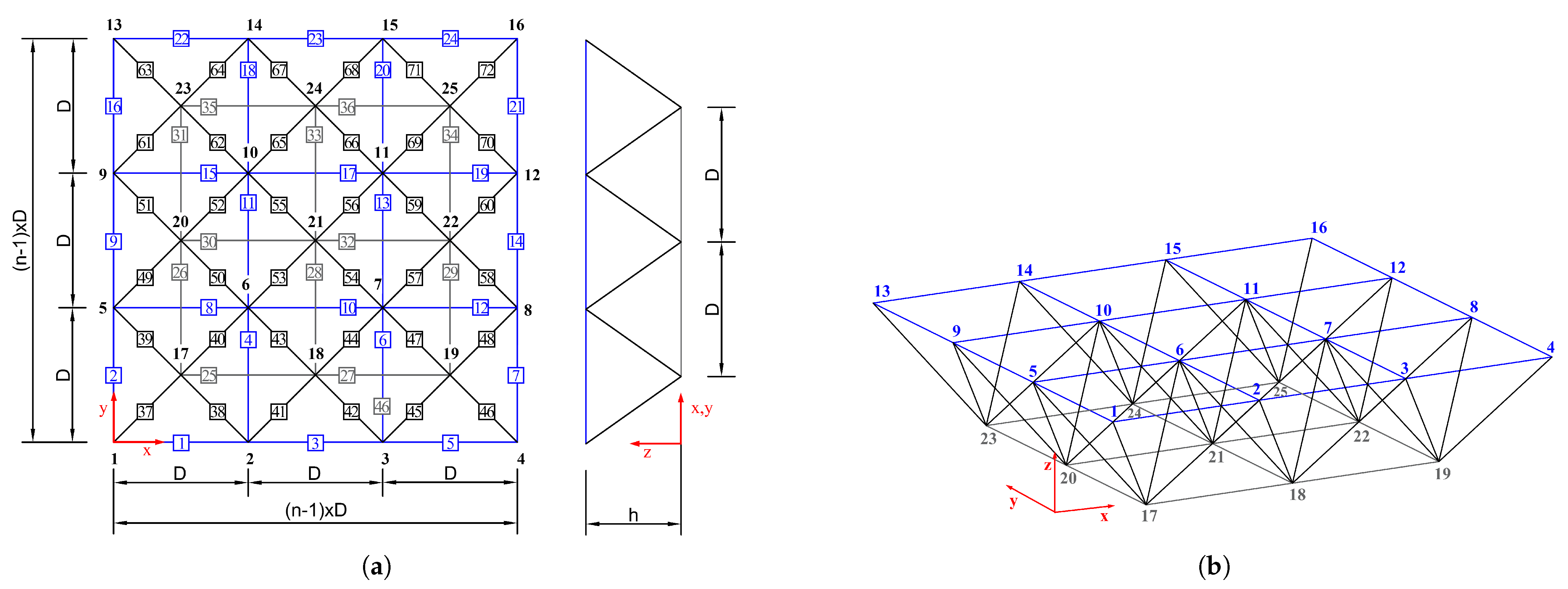
Figure 1.
Configurations of the 6-bar plane truss: (a) plan view in the x–y plane, (b) index mapping in the i–j plane.
Figure 1.
Configurations of the 6-bar plane truss: (a) plan view in the x–y plane, (b) index mapping in the i–j plane.
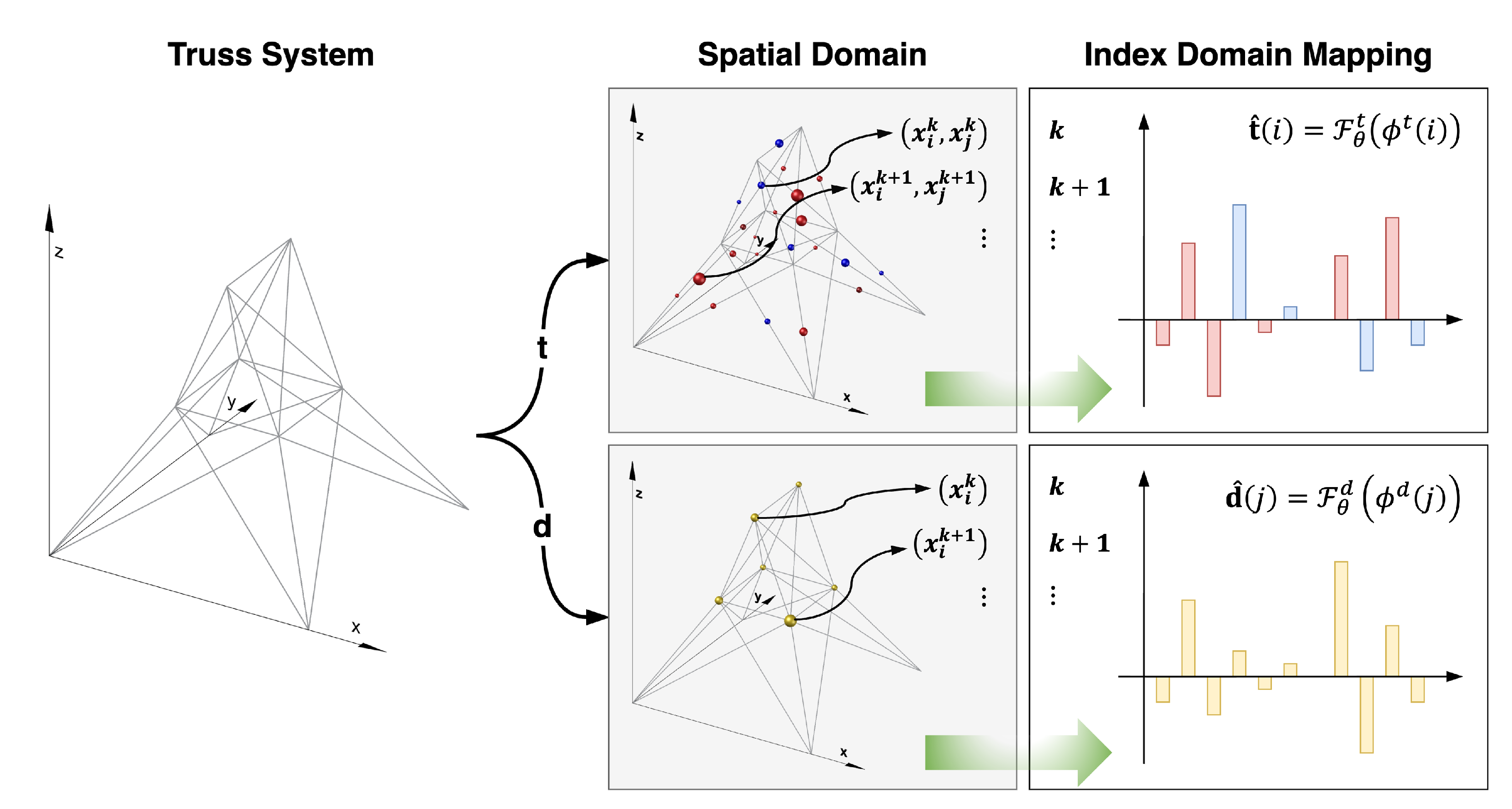
Figure 2.
Conceptual diagram illustrating the transformation of spatial domain data into the index domain in the proposed IBNN framework.
Figure 2.
Conceptual diagram illustrating the transformation of spatial domain data into the index domain in the proposed IBNN framework.
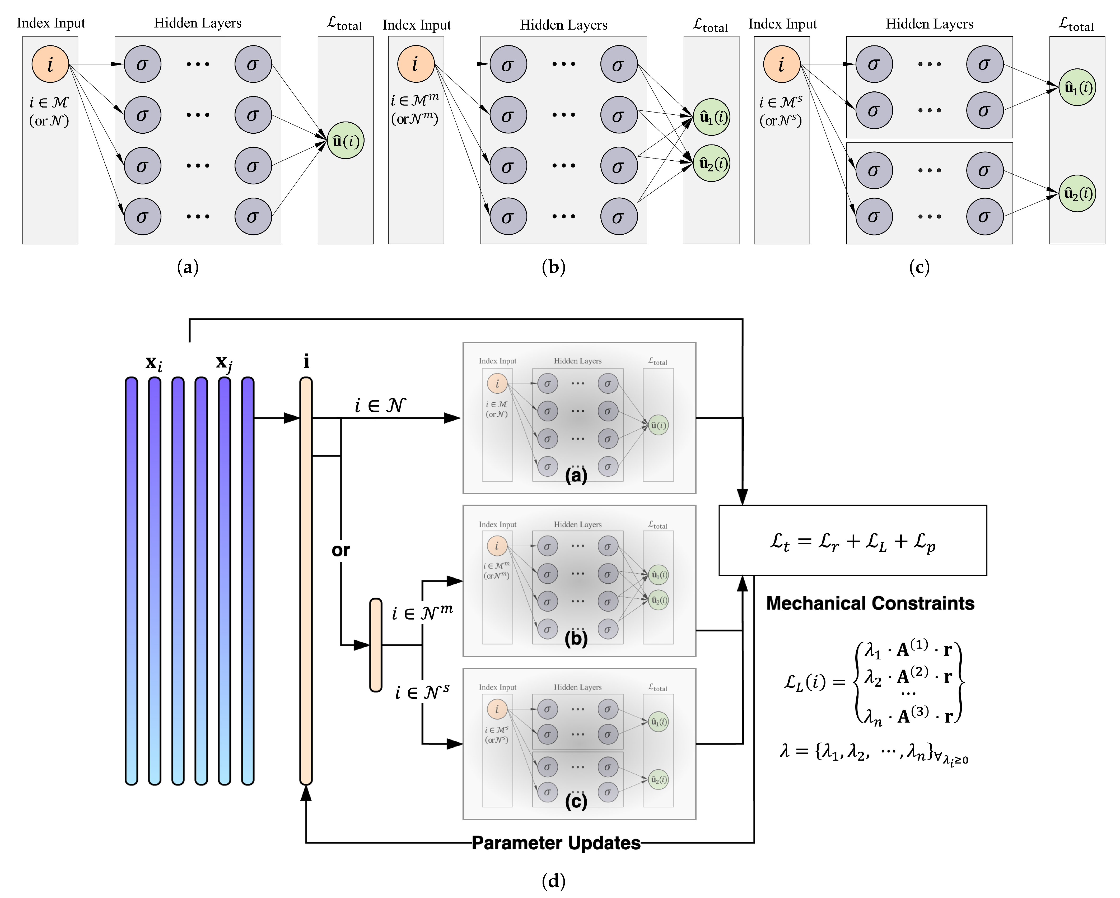
Figure 3.
Conceptual architecture of the proposed IBNN framework: (a) single-index domain, (b) multi-domain, (c) separated domain, and (d) detailed schematic of the index-based input–output structure and the computation of mechanics-informed constraints via Lagrangian multipliers under the force method formulation.
Figure 4.
Configuration of the 25-bar space truss: 3D view.
Figure 4.
Configuration of the 25-bar space truss: 3D view.
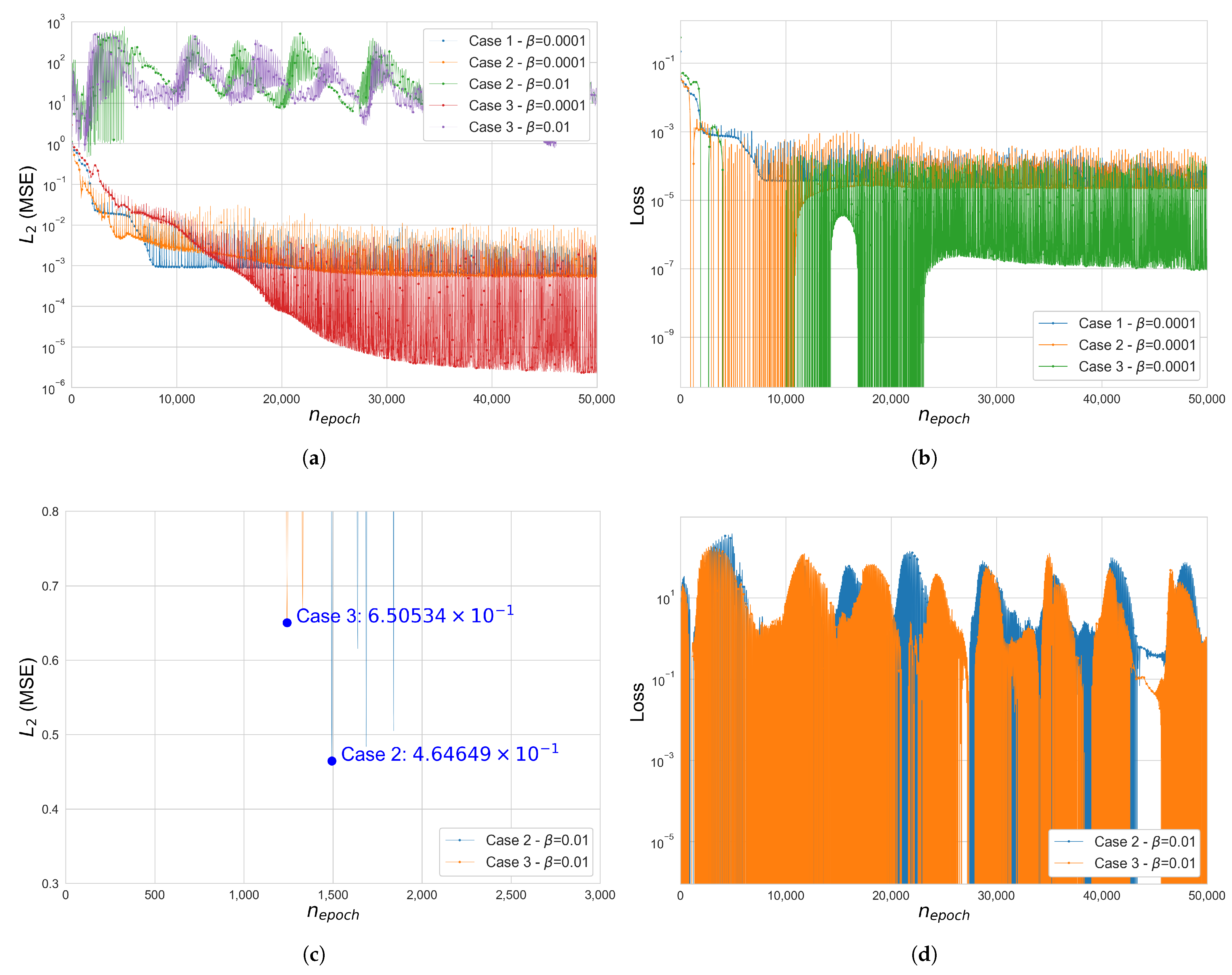
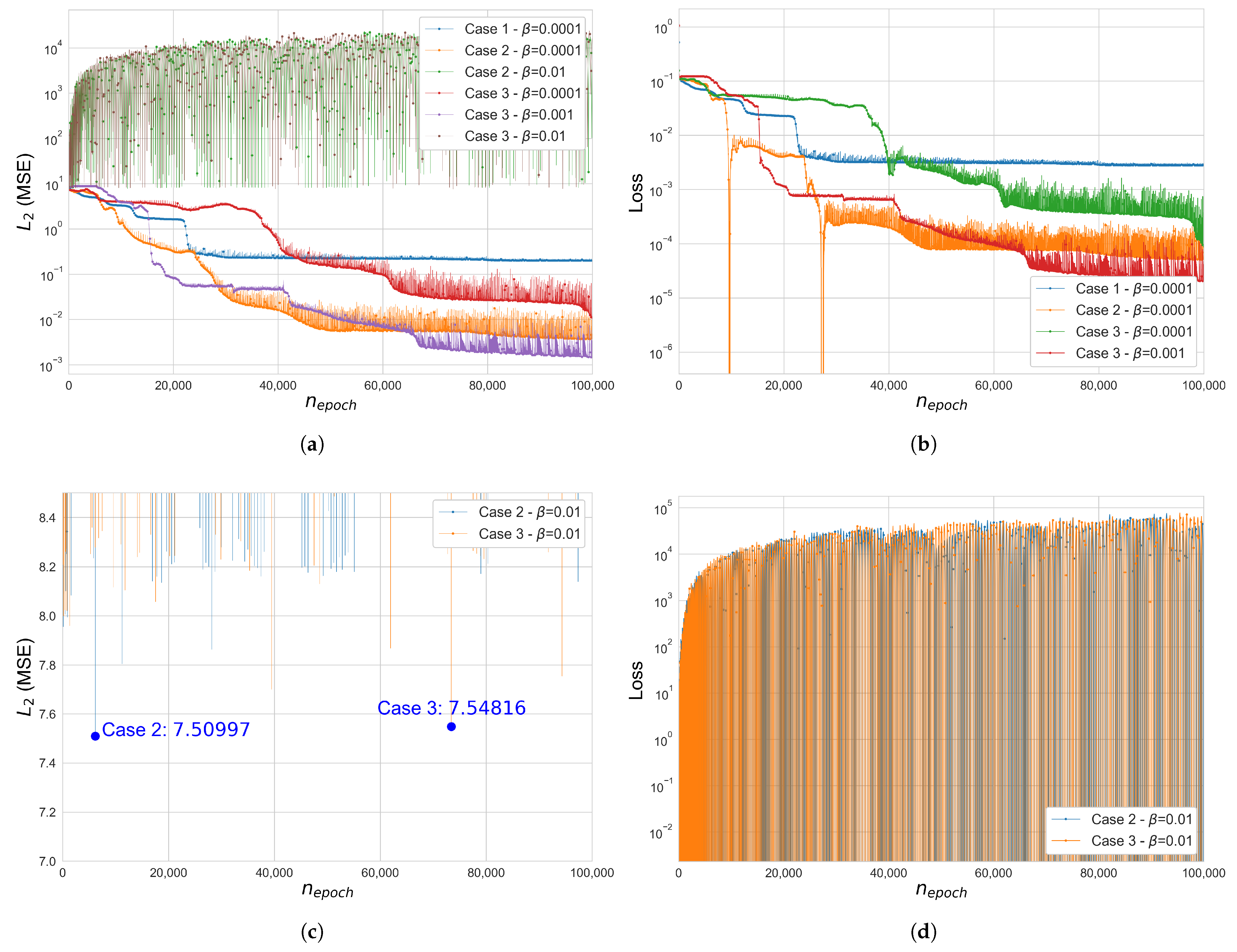
Figure 5.
Error and loss comparison for Cases 1, 2 and 3 in the 25-bar space truss (): (a) (MSE), (b) total loss function , (c) (MSE), cases 2–3, , (d) total loss , Case 2–3, . The y-axis of figures (a,b,d) is in a log scale.
Figure 5.
Error and loss comparison for Cases 1, 2 and 3 in the 25-bar space truss (): (a) (MSE), (b) total loss function , (c) (MSE), cases 2–3, , (d) total loss , Case 2–3, . The y-axis of figures (a,b,d) is in a log scale.
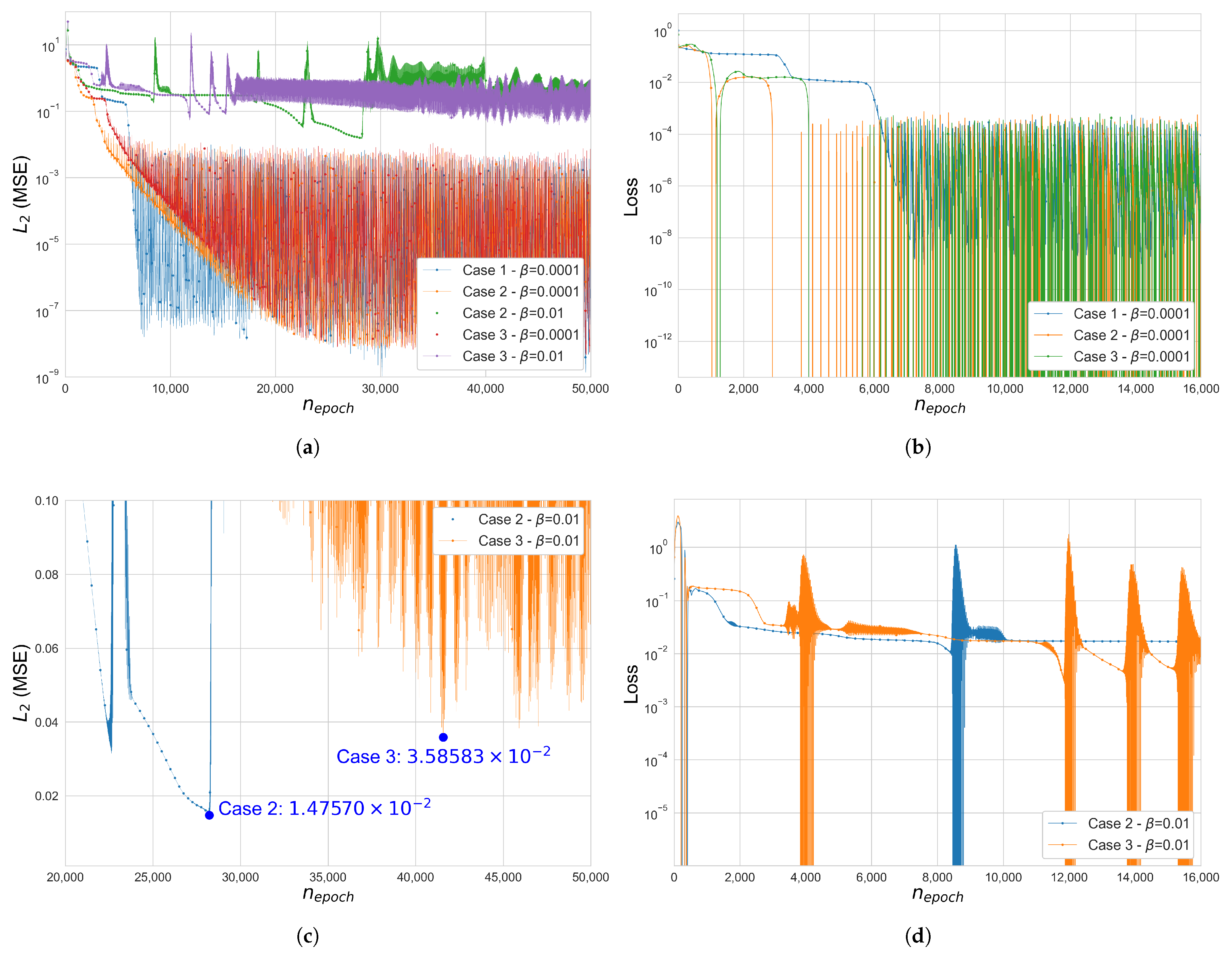
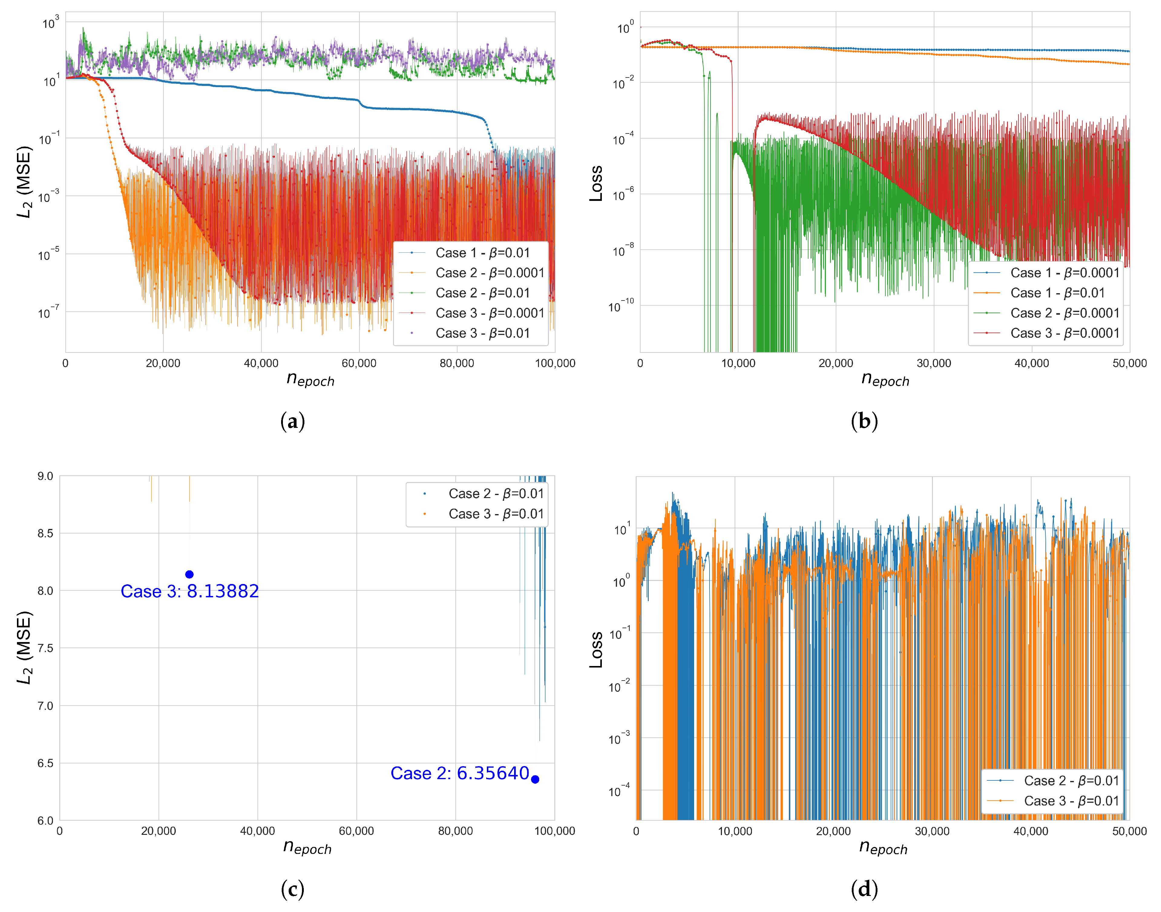
Figure 6.
Error and loss comparison for Cases 1, 2 and 3 in the 3-by-3 square grid space frame (): (a) (MSE), (b) Total loss function , (c) (MSE), Case 2–3, , (d) Total loss , Case 2–3, . y-axis of figures (a,b,d) is in a log scale.
Figure 6.
Error and loss comparison for Cases 1, 2 and 3 in the 3-by-3 square grid space frame (): (a) (MSE), (b) Total loss function , (c) (MSE), Case 2–3, , (d) Total loss , Case 2–3, . y-axis of figures (a,b,d) is in a log scale.
Figure 7.
Configurations of the 3-by-3 space frame structures: (a) plan view, (b) perspective view.
Figure 7.
Configurations of the 3-by-3 space frame structures: (a) plan view, (b) perspective view.
Figure 8.
Error and loss comparison for Cases 1, 2 and 3 in the 3-by-3 square grid space frame (): (a) (MSE), (b) total loss function , (c) (MSE), Cases 2–3, , (d) total loss , Cases 2–3, . The y-axis of figures (a,b,d) is in a log scale.
Figure 8.
Error and loss comparison for Cases 1, 2 and 3 in the 3-by-3 square grid space frame (): (a) (MSE), (b) total loss function , (c) (MSE), Cases 2–3, , (d) total loss , Cases 2–3, . The y-axis of figures (a,b,d) is in a log scale.
Figure 9.
Error and loss comparison for Cases 1, 2 and 3 in the 3-by-3 square grid space frame (): (a) (MSE), (b) total loss function , (c) (MSE), Case 2–3, , (d) total loss , Cases 2–3, . The y-axis of figures (a,b,d) is in a log scale.
Figure 9.
Error and loss comparison for Cases 1, 2 and 3 in the 3-by-3 square grid space frame (): (a) (MSE), (b) total loss function , (c) (MSE), Case 2–3, , (d) total loss , Cases 2–3, . The y-axis of figures (a,b,d) is in a log scale.
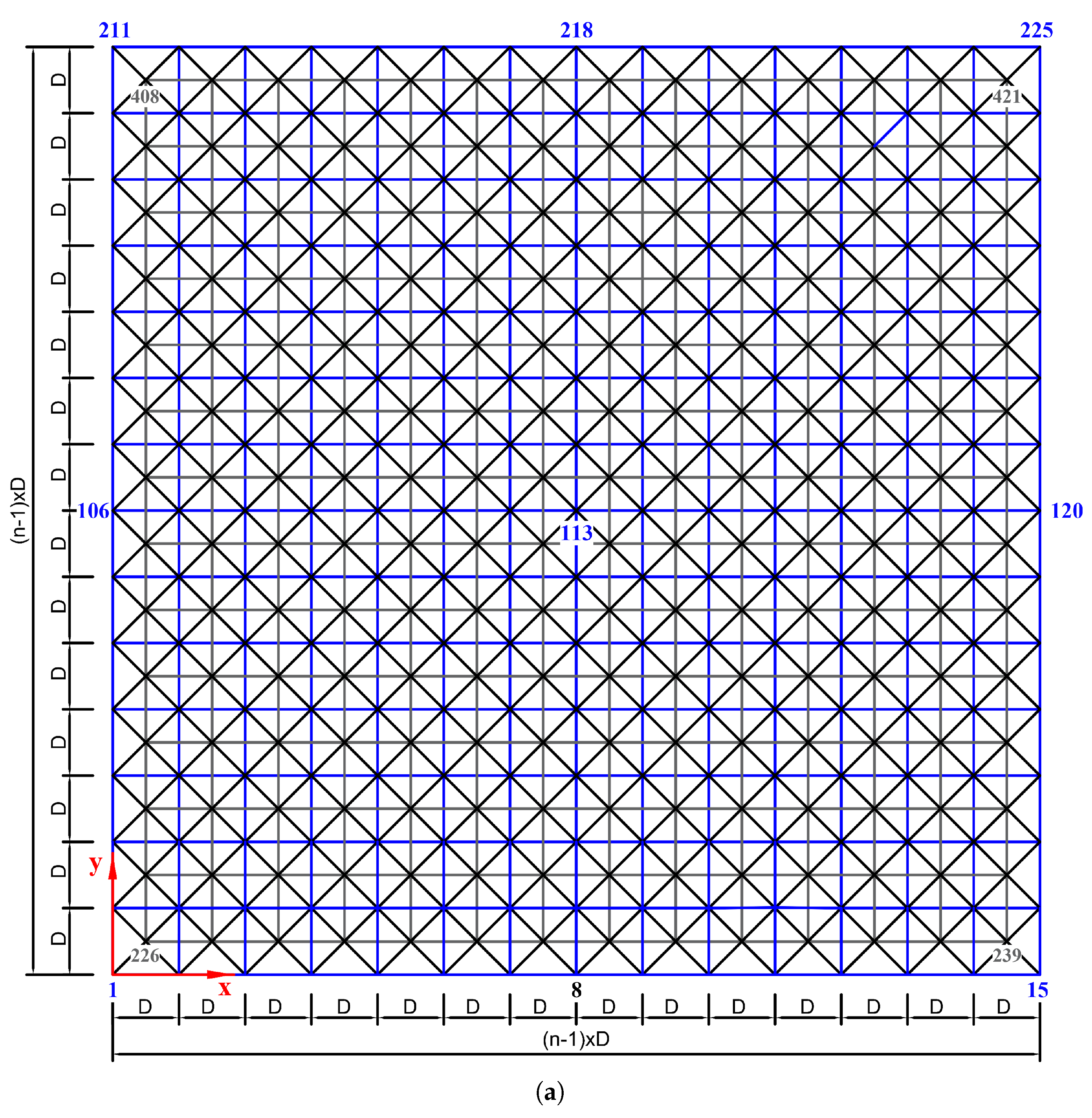
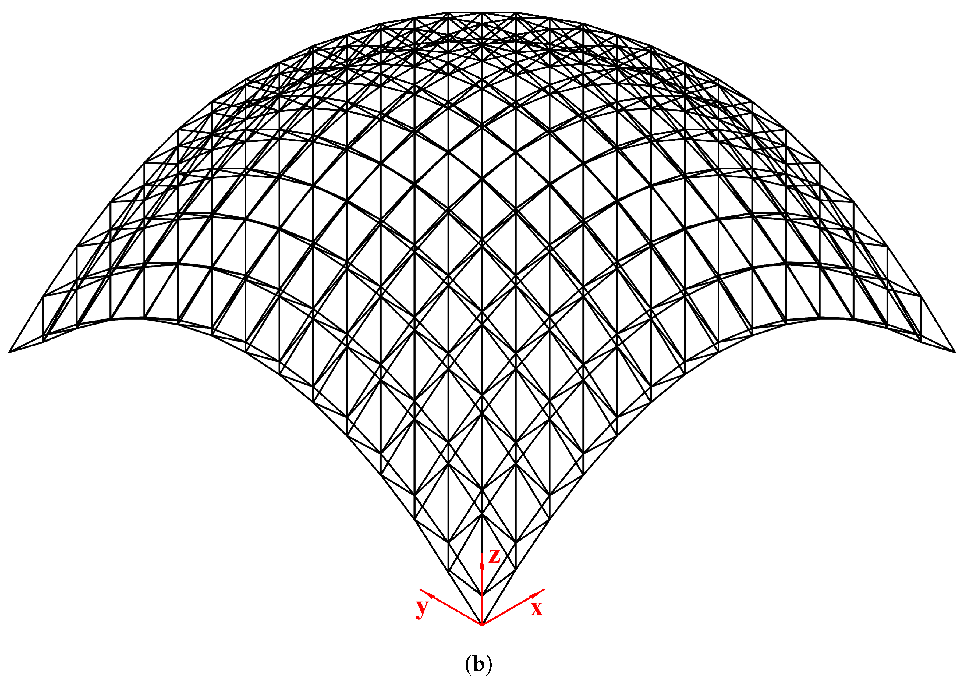
Figure 10.
Configurations of the double-layered grid dome (14-by-14): (a) plan view, (b) perspective view.
Figure 10.
Configurations of the double-layered grid dome (14-by-14): (a) plan view, (b) perspective view.
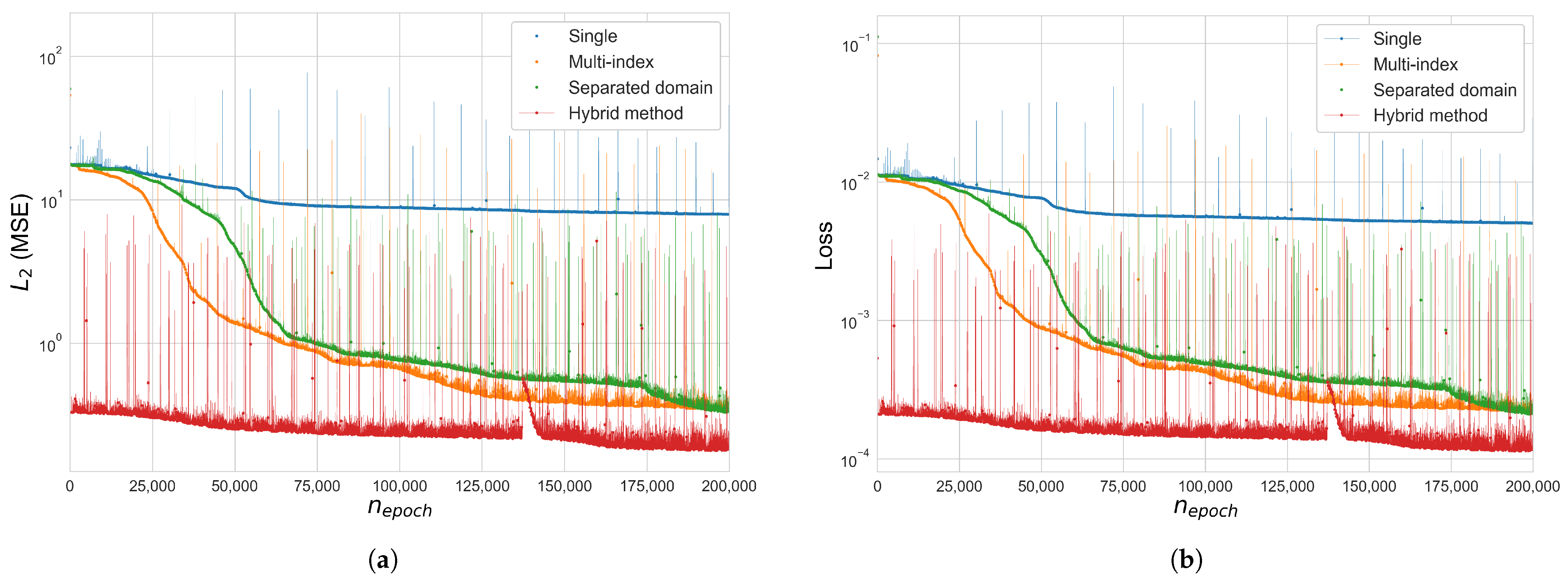
Figure 11.
Error and loss comparison for index mapping type (6-by-6 square grid space frame , and penalty method): (a) (MSE), (b) total loss function . The y-axis of the figures is in a log scale.
Figure 11.
Error and loss comparison for index mapping type (6-by-6 square grid space frame , and penalty method): (a) (MSE), (b) total loss function . The y-axis of the figures is in a log scale.
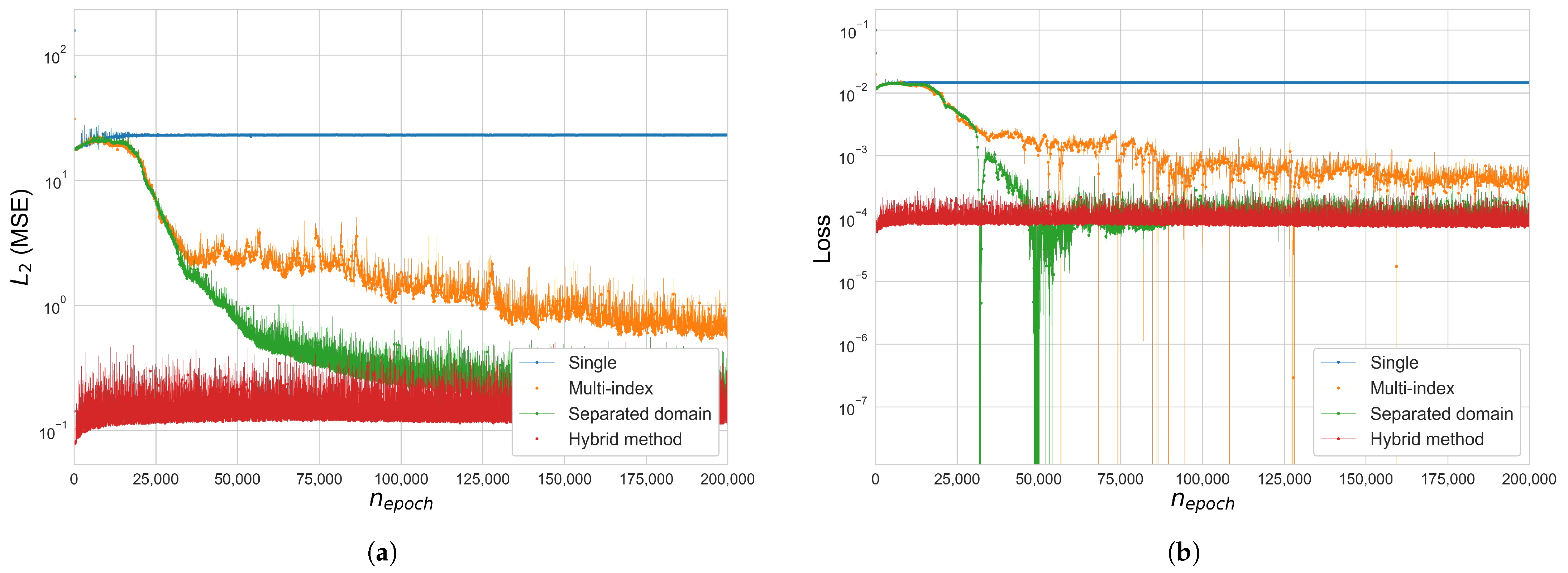
Figure 12.
Error and loss comparison for index mapping type (6-by-6 square grid space frame , and Lagrangian method): (a) (MSE), (b) total loss function . The y-axis of the figures is in a log scale.
Figure 12.
Error and loss comparison for index mapping type (6-by-6 square grid space frame , and Lagrangian method): (a) (MSE), (b) total loss function . The y-axis of the figures is in a log scale.
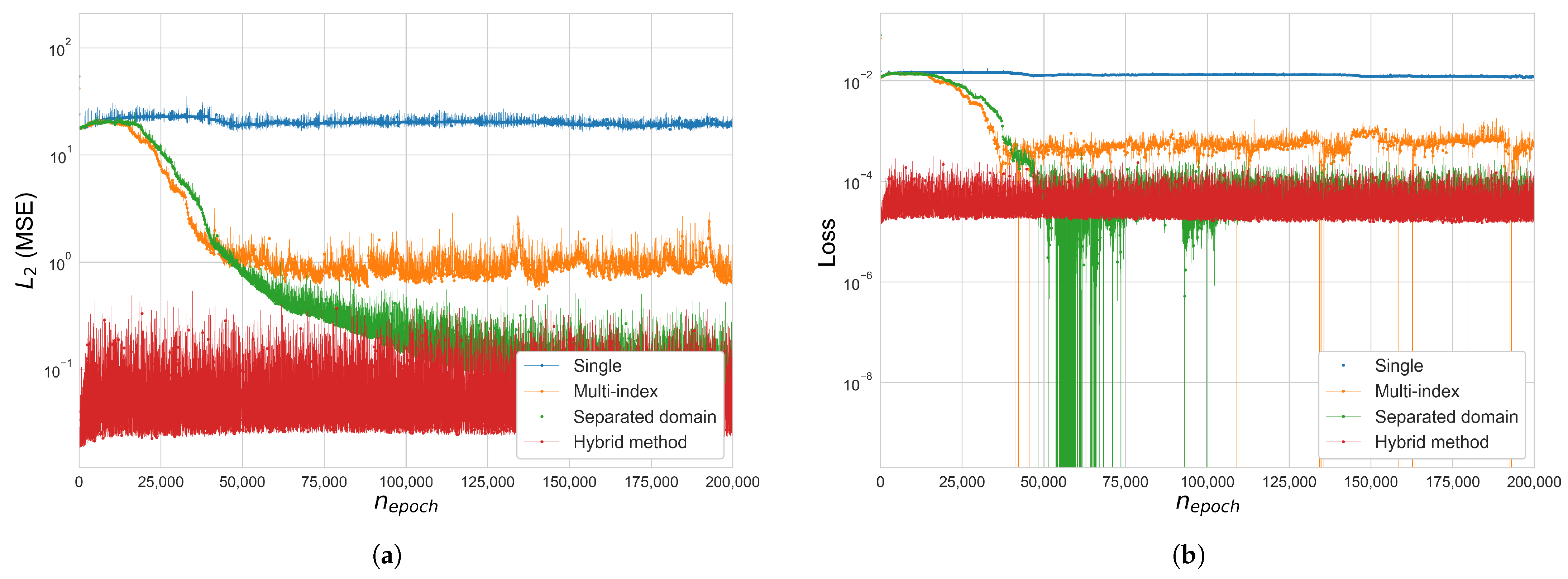
Figure 13.
Error and loss comparison for index mapping type: (6-by-6 square grid space frame , and augmented Lagrangian method): (a) (MSE), (b) total loss function . The y-axis of the figures is in a log scale.
Figure 13.
Error and loss comparison for index mapping type: (6-by-6 square grid space frame , and augmented Lagrangian method): (a) (MSE), (b) total loss function . The y-axis of the figures is in a log scale.
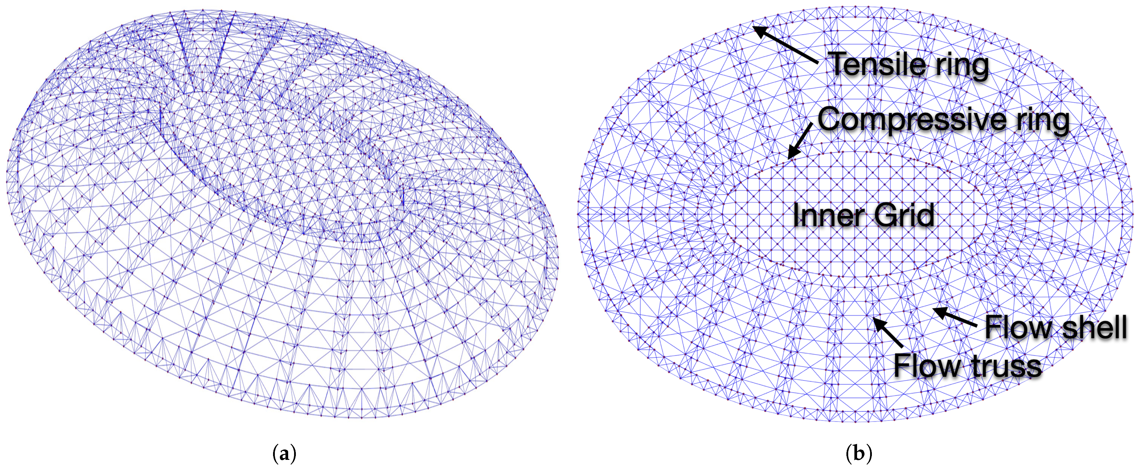
Figure 14.
Configurations of the radial flow-like truss dome (see [
71]): (
a) perspective view, (
b) plan view and model components.
Figure 14.
Configurations of the radial flow-like truss dome (see [
71]): (
a) perspective view, (
b) plan view and model components.
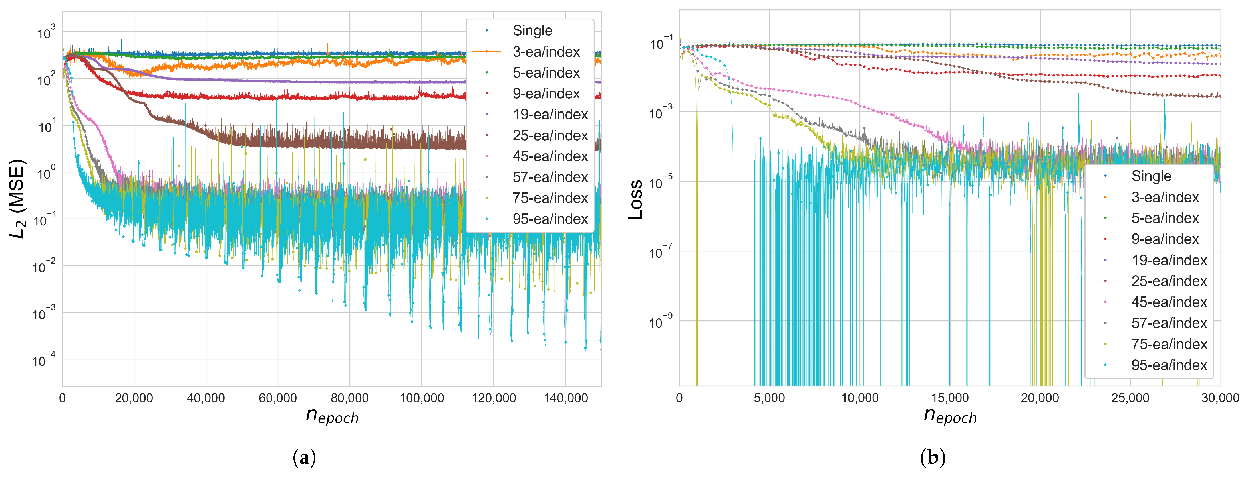
Figure 15.
Error and loss comparison of multi-domain indexing (radial flow-like truss dome ): (a) (MSE), (b) total loss function . The y-axis of the figures is in a log scale.
Figure 15.
Error and loss comparison of multi-domain indexing (radial flow-like truss dome ): (a) (MSE), (b) total loss function . The y-axis of the figures is in a log scale.
Table 1.
Comparison of total potential energy for the 6-bar plane truss obtained using coordinate-based and index-based input representations.
Table 1.
Comparison of total potential energy for the 6-bar plane truss obtained using coordinate-based and index-based input representations.
| Type of Input Domain | Ref. [62] | Coordinate (X,Y) | Index (i,j) |
|---|
| Potential energy (N·m) | −1061.228 | −1061.4184543 | −1061.4184543 |
Table 2.
Configuration of loss functions for IBNN training.
Table 2.
Configuration of loss functions for IBNN training.
| Case | Loss Function |
|---|
| Case 1 (Quadratic Penalty) | |
| Case 2 (Lagrangian) | |
| Case 3 (Augmented Lagrangian) | |
Table 3.
Comparative analysis of IBNN performance in Cases 1, 2 and 3 by (25-bar space truss ).
Table 3.
Comparative analysis of IBNN performance in Cases 1, 2 and 3 by (25-bar space truss ).
| Case | | | (MSE) | (RMSE) | | |
|---|
| Case 1: |
| | | | | | | |
| | | | | | |
| | | | | | | |
| Case 2: , |
| | | | | | | |
| | | | | | | |
| | | | | | | |
| Case 3: |
| | | | | | | |
| | | | | | | |
| | | | | | | |
Table 4.
Comparative analysis of IBNN performance in Cases 1, 2 and 3 by ∼ 0.01 (25-bar space truss ).
Table 4.
Comparative analysis of IBNN performance in Cases 1, 2 and 3 by ∼ 0.01 (25-bar space truss ).
| Case | | | (MSE) | (RMSE) | | |
|---|
| Case 1: |
| | | | | | | |
| | | | | | | |
| | | | | | | |
| Case 2: , |
| | | | | | | |
| | | | | | | |
| | | | | | | |
| Case 3: |
| | | | | | | |
| | | | | | | |
| | | | | | | |
Table 5.
Comparative analysis of IBNN performance in Cases 1, 2 and 3 by ∼0.01 (3-by-3 Square Grid Space Frame ).
Table 5.
Comparative analysis of IBNN performance in Cases 1, 2 and 3 by ∼0.01 (3-by-3 Square Grid Space Frame ).
| Case | | | (MSE) | (RMSE) | | |
|---|
| Case 1: |
| | | | | | | |
| | | | | | | |
| | | | | | | |
| Case 2: , |
| | | | | | | |
| | | | | | | |
| | | | | | | |
| Case 3: |
| | | | | | | |
| | | | | | | |
| | | | | | | |
Table 6.
Comparative analysis of IBNN performance in Cases 1, 2 and 3 by ∼0.01 (3-by-3 square grid space frame ).
Table 6.
Comparative analysis of IBNN performance in Cases 1, 2 and 3 by ∼0.01 (3-by-3 square grid space frame ).
| Case | | | (MSE) | (RMSE) | | |
|---|
| Case 1: |
| | | | | | | |
| | | | | | | |
| | | | | | | |
| Case 2: , |
| | | | | | | |
| | | | | | | |
| | | | | | | |
| Case 3: |
| | | | | | | |
| | | | | | | |
| | | | | | | |
Table 7.
Nodal coordinates in the upper layer: the eight edge nodes and top node (unit: ).
Table 7.
Nodal coordinates in the upper layer: the eight edge nodes and top node (unit: ).
| No. Node | x | y | z | Location |
|---|
| 1 | 0.0 | 0.0 | 0.0 | lower-left |
| 8 | 35.0 | 0.0 | 9.3076 | lower-middle |
| 15 | 70.0 | 0.0 | 0.0 | lower-right |
| 106 | 0.0 | 35.0 | 9.3076 | middle-left |
| 120 | 70.0 | 35.0 | 9.3076 | middle-right |
| 113 | 35.0 | 35.0 | 18.2414 | top node |
| 211 | 0.0 | 70.0 | 0.0 | upper-left |
| 218 | 35.0 | 70.0 | 9.3076 | upper-middle |
| 225 | 70.0 | 70.0 | 0.0 | upper-right |
Table 8.
Comparative analysis of IBNN performance in accordance with index mapping with
(double-layered grid dome (14-by-14) ).
Table 8.
Comparative analysis of IBNN performance in accordance with index mapping with
(double-layered grid dome (14-by-14) ).
| Case | Index-Type | | (MSE) | (RMSE) | | |
|---|
| Case 1: |
| | single | | | | | |
| | multi-index | | | | | |
| | separate | | | | | |
| | hybrid | | | | | |
| Case 2: , |
| | single | | | | | |
| | multi-index | | | | | |
| | separate | | | | | |
| | hybrid | | | | | |
| Case 3: |
| | single | | | | | |
| | multi-index | | | | | |
| | separate | | | | | |
| | hybrid | | | | | |
Table 9.
Comparative analysis of IBNN performance in Case 3 and : (radial flow-like truss dome ).
Table 9.
Comparative analysis of IBNN performance in Case 3 and : (radial flow-like truss dome ).
| Case | No. of Index Mapping | | (MSE) | (RMSE) | | |
|---|
| Case 3: |
| | 1 | | | | | |
| | 3 | | | | | |
| | 5 | | | | | |
| | 9 | | | | | |
| | 19 | | | | | |
| | 25 | | | | | |
| | 45 | | | | | |
| | 57 | | | | | |
| | 75 | | | | | |
| | 95 | | | | | |


