Article

From Signal to Safety: A Data-Driven Dual Denoising Model for Reliable Assessment of Blasting Vibration Impacts

1
College of Environment and Engineering, Hubei Land Resources Vocational College, Wuhan 430090, China
2
School of Civil Engineering & Research Center of Hubei Small Town Development, Hubei Engineering University, Xiaogan 432000, China
3
Engineering Research Center of Rock-Soil Drilling & Excavation and Protection, Ministry of Education, China University of Geosciences, Wuhan 430074, China
4
School of Information Engineering, Chang’an University, Xi’an 710064, China
*
Author to whom correspondence should be addressed.
Buildings 2025, 15(10), 1751; https://doi.org/10.3390/buildings15101751
Submission received: 25 April 2025 / Revised: 11 May 2025 / Accepted: 19 May 2025 / Published: 21 May 2025
(This article belongs to the Section Building Structures)

Abstract

With the acceleration of urban renewal, directional blasting has become a common method for building demolition. Analyzing the time–frequency characteristics of blast-induced seismic waves allows for the assessment of risks to surrounding structures. However, the signals monitored are frequently tainted with noise, which undermines the precision of time–frequency analysis. To counteract the dangers posed by blast vibrations, effective signal denoising is crucial for accurate evaluation and safety management. To tackle this challenge, a dual denoising model is proposed. This model consists of two stages. Firstly, it applies endpoint processing (EP) to the signal, followed by complete ensemble empirical mode decomposition with adaptive noise (CEEMDAN) to suppress low-frequency clutter. High-frequency noise is then handled by controlling the multi-scale permutation entropy (MPE) of the intrinsic mode functions (IMF) obtained from EP-CEEMDAN. The EP-CEEMDAN-MPE framework achieves the first stage of denoising while mitigating the influence of endpoint effects on the denoising performance. The second stage of denoising involves combining the IMF obtained from EP-CEEMDAN-MPE to generate multiple denoising models. An objective function is established considering both the smoothness of the denoising models and the standard deviation of the error between the denoised signal and the measured signal. The denoising model corresponding to the optimal solution of the objective function is identified as the dual denoising model for blasting seismic wave signals. To validate the denoising effectiveness of the denoising model, simulated blasting vibration signals with a given signal-to-noise ratio (SNR) are constructed. Finally, the model is applied to real engineering blasting seismic wave signals for denoising. The results demonstrate that the model successfully reduces noise interference in the signals, highlighting its practical significance for the prevention and control of blasting seismic wave hazards.

1. Introduction

Since the 1950s, with the progress of society and technology, the development of blasting theory and technology, and the needs of national economic development, blasting technology has been widely used in railways, highways, airports, ports and terminals, waterway regulation, water conservancy and power projects, mines, urban infrastructure construction and expansion projects, and even the medical field [1,2]. Especially in the field of directional demolition of hazardous structures, this technique offers substantial economic advantages by facilitating efficient urban renewal and infrastructure development. Nonetheless, despite the convenience that engineering blasting brings to national economic construction, the effects of blasting operations on the surrounding environment and building structures must not be overlooked. The impact of seismic effects, flying debris, air shock waves, water shock waves, dynamic water pressure, surges, toxic gases, noise, and dust pollution generated by blasting on the surrounding environment is becoming increasingly prominent. It mainly manifests as damage and cracking of existing buildings, causing property damage and quality safety accidents, slope instability and collapse, and human and animal fright. Among them, blasting seismic effects are considered the top five public hazards of engineering blasting [3,4]. Blast-induced seismic waves have emerged as a prominent human-made natural disaster, capable of causing structural damage to surrounding buildings and infrastructure.
The monitoring and analysis of blast seismic waves form the fundamental basis for hazard control. However, field-collected seismic signals are invariably contaminated with various types of noise, such as mechanical vibrations from construction equipment, ambient environmental disturbances, and electrical interference from monitoring instruments. This noise contamination significantly compromises the accuracy of vibration assessment and subsequent safety evaluations, and under poor monitoring conditions, there are even instances where the actual signal is completely submerged by noise [5,6]. Time–frequency analysis is currently the most widely used method for analyzing blasting seismic waves; however, noise can significantly impair the accuracy of time–frequency analysis results [7,8,9]. The primary issue is that empirical mode decomposition (EMD) can lead to serious mode confusion when influenced by noise [10]. Enhancing empirical mode decomposition through ensemble empirical mode decomposition (EEMD) and complementary ensemble empirical mode decomposition (CEEMD) might compromise the integrity of the original signal due to the addition of white noise [11,12,13]. Consequently, the most prevalent method at present is complete ensemble empirical mode decomposition with adaptive noise (CEEMDAN). This algorithm employs adaptive white noise to counteract the noise present during monitoring, suppressing modal mixing while preserving the authenticity of the original signal [14].
The noise reduction processing of blasting seismic wave signals may seem unrelated to the damage caused by blasting to building structures, but it is actually the foundation for reducing the risk of human-made natural disasters such as seismic waves from blasting [15].
Blasting seismic signals exhibit instantaneous, abrupt, and oscillatory characteristics, and they are classified as typical nonstationary signals. Currently, commonly used denoising methods for blasting seismic wave signals include wavelet and wavelet packet threshold denoising [16,17,18]. The theoretical foundation of the wavelet transform is the Fourier transform, which inherently leads to the limitations of using Fourier analysis for nonstationary signals, including the generation of spurious frequencies and redundant signal components [19,20,21]. EMD denoising [22,23], improved EMD denoising [24,25,26,27,28], wavelet threshold EMD denoising [29,30], and threshold control-improved EMD denoising [31,32], among others. These methods yield certain effects on the noise reduction processing of blasting seismic wave signals, particularly the threshold control-improved EMD blasting seismic wave noise reduction processing method. This method integrates the adaptability of enhanced EMD with the capability to implement threshold-based low-pass filtering, leveraging the strengths of both techniques. Consequently, it has been extensively utilized in the noise reduction of blast-induced seismic waves. EMD is extensively applied in the domain of nonlinear and nonstationary signal processing because it analyzes data according to its intrinsic properties.
Considering that signals may exhibit varying degrees of divergence at both ends due to endpoint effects, the shorter the data, the greater the impact of signal endpoint effects. The denoising algorithm may also be affected by endpoint effects at the signal endpoints, which can affect the denoising effect of the algorithm. Therefore, based on the threshold control-improved EMD denoising algorithm, this paper introduces an endpoint processing program to mitigate the interference of endpoint effects on the denoising effect of the model and to better achieve the denoising processing of blasting seismic wave signals [33]. By adding an endpoint processing algorithm on the basis of threshold control-improved EMD denoising processing, the first stage of denoising can be achieved. The second stage of noise reduction processing involves solving the optimal value problem in advanced mathematics. Only by completing these two steps can the denoising model for blasting seismic wave signals proposed in this paper be realized.
The evaluation of the model’s denoising performance is conducted using simulated blasting vibration signals with a specified signal-to-noise ratio (SNR). By comparing the standard deviation of the error between artificially generated noise-free signals and the denoised signals, the denoising effectiveness can be assessed. Furthermore, the model’s capacity to maintain the true characteristics of the original monitoring signals can be evaluated. This denoising model is applicable to real engineering blasting vibration signals and nonstationary vibration signals affected by noise interference. It eliminates distortions in time–frequency analysis caused by noise and endpoint effects, providing robust support for the in-depth exploration of blasting seismic wave vibration characteristics and the control of blasting seismic wave hazards [34]. This study concentrates on noise reduction processing of blasting seismic wave signals to enhance signal quality and improve the accuracy of structural risk assessment. Further research is required to investigate the application of this denoising model in other nonlinear signal denoising processes.

2. Method

This section provides a detailed explanation of the process of establishing the denoising model for blasting seismic wave signals, which consists of two stages.

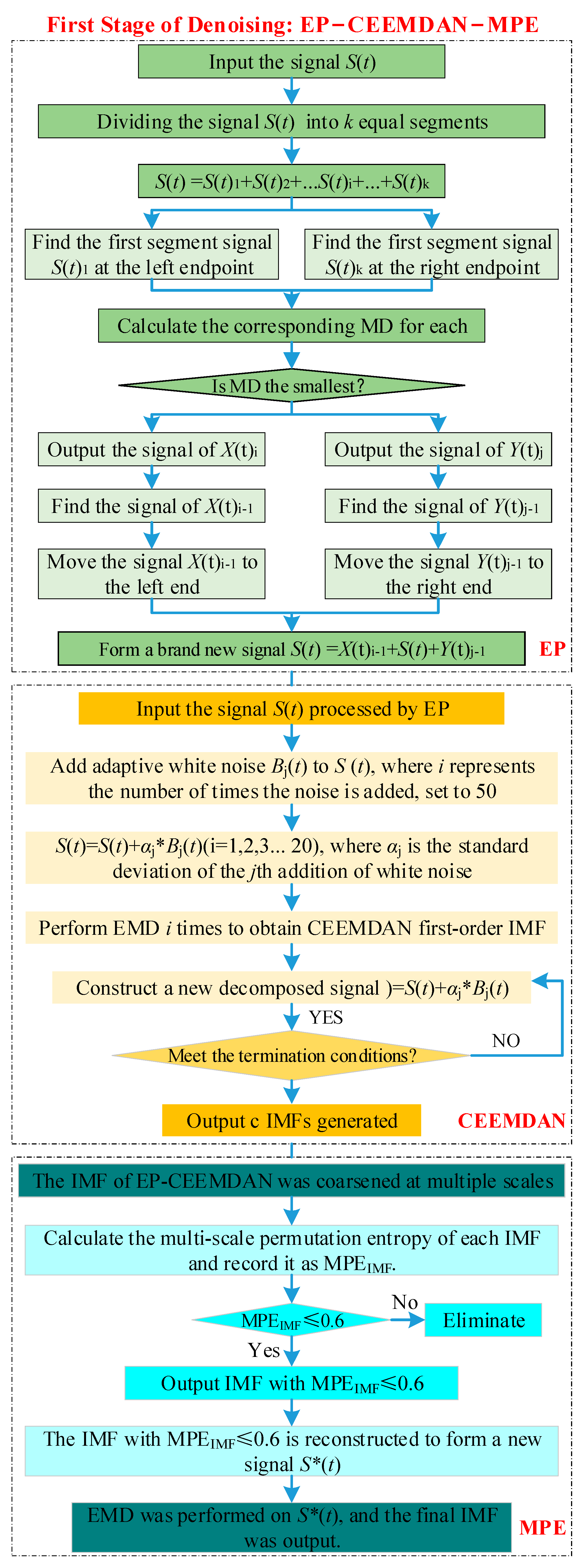
2.1. First Stage of Denoising: EP-CEEMDAN-MPE

2.1.1. Endpoint Processing (EP)

The endpoint effect is an almost unavoidable issue in most denoising algorithms. Signals often diverge at their endpoints, and this phenomenon becomes more pronounced with shorter data lengths. The denoising algorithm proposed in this paper incorporates an endpoint processing procedure to mitigate the impact of endpoint effects on denoising performance. The specific implementation is as follows.
The trend of a signal is reflected not only at its endpoints but also within the signal itself. By dividing the signal S(t) into k equal segments, we obtain S(t) = S(t)1 + S(t)2 + …S(t)i… + S(t)k. Taking the left endpoint S(t)1 as a reference, a segment within S(t) that exhibits the highest matching degree (MD) with S(t)1 is identified, denoted as X(t)i. Using X(t)i as a reference, X(t)i−1 is identified and translated to the left endpoint of the signal.
The calculation of matching degree is shown in Equation (1), where d is the linear normalized result of the sum of distances between any two points on S(t)1 and S(t)i (2 ≤ ik), as calculated in Equation (2). The correlation coefficient r is calculated by Equation (3). Since the development trend of the signal is reflected not only at the endpoints but also within the signal itself, it is evident that r > 0.
MD = d r
d = i = 2 k S t 1 S t i i = 2 k S t 1 S t i max
r = cov S t 1 , S t i σ S t 1 σ S t i
To better quantify the matching degree between two waveforms, the matching degree formula (Equation (1)) is introduced. This formula comprehensively considers two metrics: amplitude and waveform similarity. A smaller d indicates that the amplitudes of the two signals are closer, while a larger r signifies greater similarity between the two signals. Therefore, for the matching degree, a smaller value indicates a higher degree of matching between the two signals, and vice versa. Our goal is to identify the X(t)i, that exhibits the highest matching degree with S(t)1. Using X(t)i as a reference, X(t)i−1 is shifted to precede the left endpoint S(t)1, forming a new left endpoint.
Similarly, for the right endpoint, the right endpoint S(t)k is used as a reference to identify a segment within S(t) that exhibits the highest matching degree (MD) with S(t)k, denoted as Y(t)j. Using Y(t)j as a reference, Y(t)j+1 is identified and translated to the right endpoint of the signal. Through this endpoint processing, the signal S(t) is transformed into X(t)i−1 + S(t) + Y(t)j+1, effectively extending the signal at both endpoints using subsequences guided by the “internal development trend” of the signal.
The denoising process is then applied to the signal X(t)i−1 + S(t) + Y(t)j+1. During computation, S(t) is redefined as X(t)i−1 + S(t) + Y(t)j+1. By studying the denoising performance of S(t), the interference from endpoint effects on the denoising results can be effectively mitigated.

2.1.2. CEEMDAN-MPE

The CEEMDAN-MPE algorithm enhances the complete ensemble empirical mode decomposition with adaptive noise (CEEMDAN) [35] by integrating a multi-scale permutation entropy (MPE) procedure [36,37]. Initially, the signal is subjected to endpoint processing (EP), succeeded by CEEMDAN decomposition. Subsequently, the permutation entropy values of the intrinsic mode functions (IMFs) derived from EP-CEEMDAN are computed. Only those IMFs that satisfy the predefined entropy criteria are selected for output.
MPE is an optimization method of combining multiple scales with permutation entropy (PE) [38]. It can analyze time series more efficiently.
Suppose the length of any one-dimensional time series x(i) is L. X(i) can be expressed as: xL(i) = {x1,x2,x3xL}. The Equation (4) is obtained by coarsening xL(i) with multi-scale coarsening.
y j s = 1 s i = ( j 1 ) s + 1 j s x i , 1 j L s
In Equation (4), s is the scale factor and ysj is the multi-scale time series. By replacing the IMF obtained from EP-CEEMDAN with ysj, a multi-scale IMF can be obtained. By calculating the PE of the multi-scale IMF, the MPE of the IMF can be obtained.
According to the definition of MPE [39,40], when the MPE of IMF is greater than 0.6, it can be considered as an abnormal component with great randomness and needs to be eliminated.
CEEMDAN introduces a finite amount of adaptive white noise at each stage, enabling nearly zero reconstruction errors with fewer averaging iterations. Its inherent adaptability makes it particularly effective in suppressing low-frequency clutter. The specific steps are as follows:
Step 1: Add the adaptive white noise Bj(t) to the signal S(t) after the EP, where j is the number of times to add the noise, 20 times in this paper. Then the signal of the jth order can be expressed as S(t) = S(t) + αj*Bj(t) (j = 1,2,3…20), where α is the standard deviation of the jth white noise addition. For the IMF1 obtained by EP-CEEMDAN, see Equation (5), the remainder is R(t) = S(t)-IMF1.
IMF 1 = 1 i i = 1 20 I M F i
Step 2: Construct a new signal S(t) = S(t) + αj*Bj(t) and decompose 20 times. The IMF2 is obtained, and the remainder is R(t) = S(t)-IMF2.
Step 3: Repeat “Step 1” and “Step 2” until the end of the program. S(t) obtains c IMF and the unique remainder R(t) through CEEMDAN. The decomposition result is shown in Equation (6).
R t = S t i = 1 c I M F c
Compared to PE, MPE offers the advantage of multi-scale coarse-graining. This process involves segmenting the time series (specifically, the IMFs obtained from EP-CEEMDAN) and averaging within each segment, thereby enhancing processing precision. By setting a permutation entropy threshold, the entropy of the processed time series is controlled, effectively suppressing high-frequency noise that is mixed into the vibration signals during monitoring.

2.1.3. EP-CEEMDAN-MPE

To better understand the algorithmic principle of the first stage of denoising, we draw a flowchart of the EP-CEEMDAN-MPE, as depicted in Figure 1.

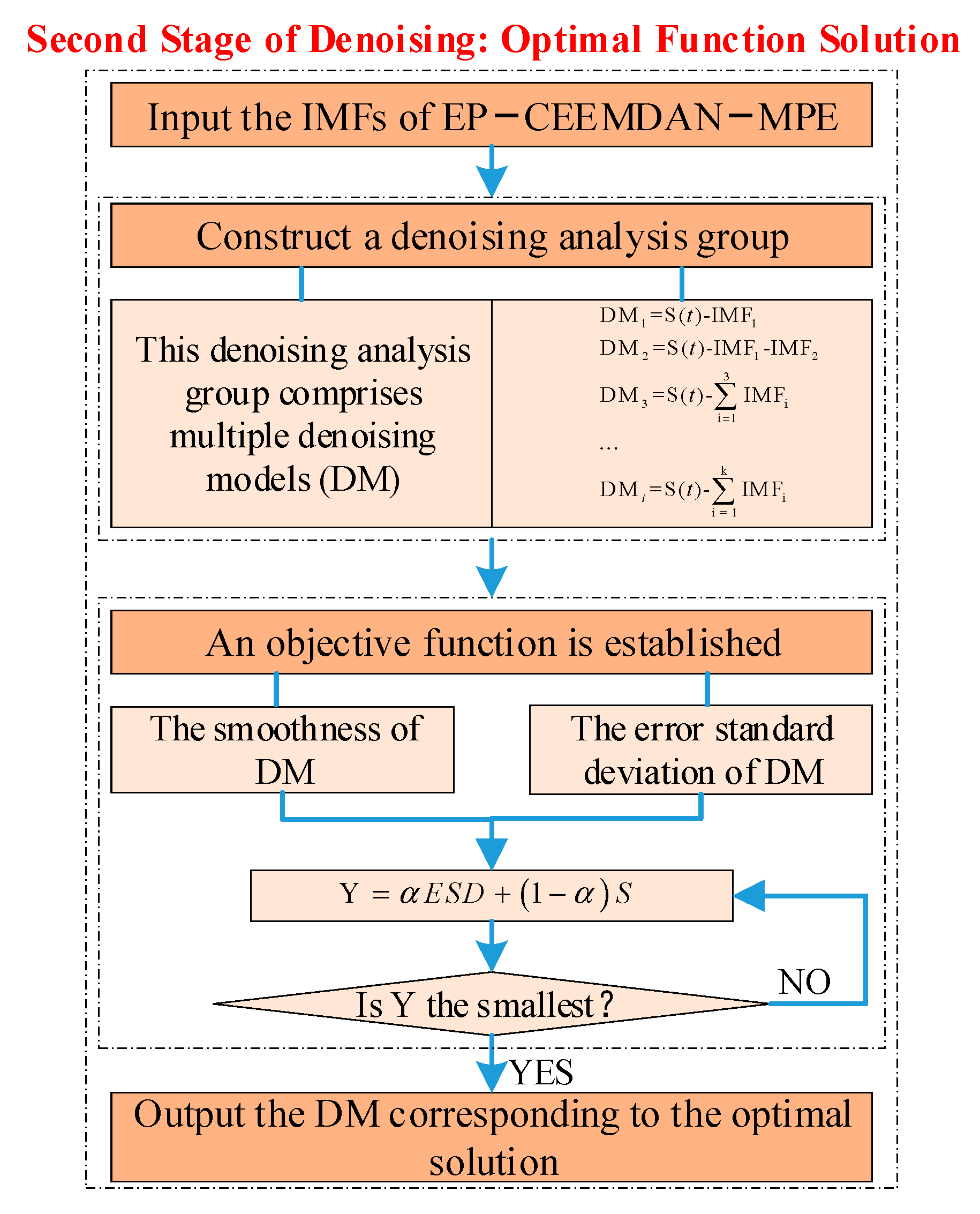
2.2. Second Stage of Denoising: Optimal Function Solution

2.2.1. Construction of the Denoising Analysis Group

The IMFs obtained from EP-CEEMDAN-MPE are combined using Equation (7) to construct a denoising analysis group. This group comprises multiple denoising models (DMs), each of which can be expressed by Equation (8). By examining Equations (7) and (8), it is evident that the signal processed through EP-CEEMDAN-MPE yields k IMFs and a unique residual term R(t).
S ( t ) = i = 1 k I M F i + R t
D M i = S ( t ) - i = 1 k I M F i

2.2.2. Optimal Function Solution

The process of identifying the DM with the optimal denoising performance within the denoising analysis group is achieved through the solution of an optimal function. The function parameters are determined based on two key considerations:
  • Protection of the true components of the original signal: This is quantified by the error standard deviation (ESD) between the DM and the original signal.
  • Degree of denoising: This is reflected by the smoothness (S) of the DM.
An objective function is established considering both the S of the DM and the ESD between the DM and S(t). The DM corresponding to the optimal solution of this objective function is identified as the desired DM.
A weighting coefficient β is introduced, and the objective function Y can be expressed by Equation (9). Here, the ESD between the DM and the original signal is defined by Equations (10). In Equation (10), N represents the total number of sampling points in the original signal.
Y = β E S D + 1 β S
E S D = S t D M 2 N
The smoothness of the DM is established as follows.
The smooth curve f(x) can be derived at any point of the curve, and the IMF component with noise cannot meet this condition, so the core of denoising is to smooth the curve. According to the necessary and sufficient conditions of function derivability, any smooth curve satisfies Equation (11).
f x 0 = lim h 0 f x 0 + h f x 0 h = f + x 0 = lim h 0 + f x 0 + h f x 0 h
In Equation (11), x0 denotes any arbitrary point within N, and h is the sampling interval. If f(x) is composed of two or more curves, f(x) satisfies Equation (12).
f x = u x < x w 0 v x w 0 x < +
Then f(x) satisfies Equation (13).
u w 0 = lim h 0 u w 0 + h u w 0 h = v + w 0 = lim h 0 + v w 0 + h v w 0 h
u-(w0) is the left limit of u(x) at w0 and v + (w0) is the right limit of v(x) at w0. Because the curve is smooth at w0, u(x) and v(x) have the same curvature at w0, which satisfies Equation (14).
K u | w = w 0 = u x 0 1 + u x 0 2 3 2 = K v | w = w 0 = v x 0 1 + v x 0 2 3 2
In the Equation (14), Ku|w=w0 and Kv|w=w0 are the curvatures of u(x) and v(x), respectively.
According to Equation (14), we can obtain Equation (15).
u w 0 = v w 0
u’’(w0) and v’’(w0) are the second derivatives of u(x) and v(x) at w0. We calculate u’’(w0) and v’’(w0), respectively, to obtain Equations (16) and (17).
v w 0 = v w 0 + h v w 0 h = l i m h 0 v w 0 + 2 h 2 v w 0 + h + v w 0 h 2
u w 0 = u w 0 + h u w 0 h = l i m h 0 u w 0 + 2 h 2 u w 0 + h + u w 0 h 2
According to Equations (15) to (17), Equation (18) can be obtained.
S | x = x 0 = f x 0 + 2 h f x 0 2 h 2 f x 0 + h f x 0 h
By replacing f(x) with DM, we can obtain Equation (19) for the smoothness of the DM
S | x = x 0 = D M x 0 + 2 h D M x 0 2 h 2 D M x 0 + h D M x 0 h
The ESD between the DM and the original signal controls the degree of deviation between the two. A smaller ESD indicates that the DM preserves more of the original signal’s characteristic components. The S of the DM serves as an indicator of the denoising intensity. According to the literature, the smoother the curve at a given point, the smaller the value of S and the higher the denoising intensity of the model at that point.
Therefore, when the objective function reaches its minimum value, the optimal solution is obtained. The DM corresponding to this optimal solution is identified as the dual-stage denoising model.
To better understand the algorithm principle of the second stage of denoising, we draw a flowchart of the optimal function solution, as shown in Figure 2.

3. Evaluation of the Denoising Performance of the Denoising Model

3.1. Generation of Simulated Blasting Vibration Signals with a Given Signal-to-Noise Ratio

To evaluate the denoising performance, a noise signal n(t) with a specified signal-to-noise ratio (SNR) is generated. A noise-free sinusoidal signal x(t)= sin(2 × π × 100 × t) is constructed, where N = 1000 and t = 1/N:1/N:1. A random noise vector of size 1 × 1000 is generated and standardized to have a mean of 0 and a variance of 1. The effective power of the signal (Ps) is calculated as 0.5000.
Given a signal-to-noise ratio (SNR = 10), the effective power of the noise (Pn) is calculated as 0.0500. The random noise is then scaled to have a mean of 0 and a variance of Pn = 0.0500, resulting in the noise signal n(t) with the specified SNR = 10.
The signals x(t), n(t), and S(t) = x(t) + n(t) are plotted, as shown in Figure 3.

3.2. Construction of the Denoising Model for Simulated Signals

To highlight the endpoint processing effect, EP-CEEMDAN-MPE and CEEMDAN-MPE were compared and analyzed for S(t), and the results are shown in Figure 4 and Figure 5, respectively.
From Figure 4, it can be observed that each IMF follows the original trend at the endpoints without exhibiting endpoint divergence. This demonstrates that the endpoint processing effectively preserves the authenticity of the original signal and eliminates the interference of endpoint divergence during denoising. Additionally, the decomposition results are arranged from high to low frequencies, and the mode confusion phenomenon commonly associated with EMD is effectively suppressed. While IMF1 exhibits slight mode confusion, the remaining components are relatively stable.
Comparing Figure 4 and Figure 5, it is not difficult to see that there is severe confusion in the mid- to high-frequency modes, especially in IMF1, where there is a trend towards low-frequency development at both the endpoints and within the signal. Next is the right endpoint of IMF4, which shows a clear trend towards lower frequencies. The low frequency is relatively stable, and there is no obvious mode confusion. Comparing Figure 4 and Figure 5, it can be found that endpoint processing is very necessary.
Observing Figure 4, it can be found that S(t) obtained seven IMFs and one remainder R(t) through EP-CEEMDAN-MPE. Based on Equation (8), a DM for the simulated signal is established, as shown in Equation (20).
D M 1 = S t i = 1 1 I M F i D M 2 = S t i = 1 2 I M F i D M 7 = S t i = 1 7 I M F i
Using Equations (10) and (19), the ESD between S(t) and each denoising model (DM1, DM2, …, DM7) as well as the S of each denoising model (DM1, DM2, …, DM7) are calculated. The results are then linearly standardized.
Since the primary goal of denoising is to facilitate better analysis of blasting vibration characteristics, the authenticity of the original signal must be preserved. Therefore, β is set to be greater than 0.5. However, it is also important to avoid solely focusing on the reconstruction error standard deviation between the DM and S(t) while neglecting the denoising effect. Thus, the final range for β is chosen as 0.5 < β < 0.9.
Table 1 lists the relevant parameter values of the objective function for 0.5 < β < 0.9, with the optimal DM corresponding to different values of β highlighted in bold.
From Table 1, the following conclusions can be drawn:
(1)
As β increases, Y increases. When β = 0.6, the optimal function reaches its minimum value of 0.1578, and the denoising model is identified as DM2.
(2)
From DM1 to DM7, the reconstruction ESD between the DM and S(t) gradually increases, indicating a higher degree of denoising. However, DM7 shows poor correlation with the original signal, resulting in over-denoising.
(3)
Critical state: When β = 0.8845, the DM no longer has a unique solution.
To highlight the differences between the DM and the noisy signal, the comparison between S(t) and the DM is illustrated for β = 0.7, as shown in Figure 6. Figure 6 clearly demonstrates that DM5, DM6, and DM7 exhibit over-denoising, leading to distortion in the DM. The optimal denoising model, DM2, effectively preserves the authentic information of the original signal while achieving smooth denoising. This analysis aligns with the results obtained from solving the optimal equation in Table 1, reflecting the scientific validity and correctness of the optimal denoising model.

3.3. Evaluation of Denoising Performance for Simulated Signals

The evaluation of denoising performance serves two purposes:
(1)
It assesses the denoising capability of the DM.
(2)
It validates the correctness of the optimal equation solution (using β = 0.7 as an example).
The denoising performance of the DM is evaluated using the signal-to-noise ratio (SNR), as expressed in Equation (21).
S N R = 10 log 10 P s P n
The effective power of the signal (Ps) is calculated as 0.5000. Given a signal-to-noise ratio (SNR = 10), the effective power of the noise (Pn) is calculated as 0.0500. It is not difficult to find that the difference between the power of the denoising model (PDM) and Pn is the reduced noise power (PDM − Pn), and (PDM − Pn) ≤ Pn is satisfied.
In order to measure the denoising effect of the DM, Equation (21) needs to be rewritten to obtain an improved signal-to-noise ratio (ISNR) calculation in Equation (22).
I S N R = 10 log 10 P s P D M P n
According to the definition of the logarithmic function, ISNR > SNR > 10. The greater the difference between ISNR and SNR, the more pronounced the denoising effect of the model. The calculated ISNR values are presented in Table 2.
From Table 2, it can be observed that the ISNR values for DM4 to DM7 cannot be calculated because the logarithm function becomes undefined when its argument is less than zero. This occurs if and only if PDM < 0.5000, indicating that the argument of the logarithm is negative. This implies that the DM fails to preserve the authenticity of the sinusoidal signal, as over-denoising leads to model distortion. Therefore, only the denoising performances of DM1 to DM3 are compared here.
As previously analyzed, the greater the difference between ISNR and SNR, the more significant the denoising effect of the model. From Table 2, it is evident that the denoising model DM2 (using β = 0.7 as an example) exhibits the optimal denoising performance. This result aligns with the optimal solution of the objective function (using β = 0.7 as an example) in Section 3.2 and the DM comparison in Figure 6. This consistency further demonstrates that the proposed optimal denoising model achieves excellent denoising performance, and its formulation is scientifically sound.

3.4. Analysis of Noise Reduction Results of Simulated Blasting Vibration Signals

1.
Simulated signal generation and denoising model construction occurred as follows:
(1)
A simulated blasting vibration signal S(t) with a specified signal-to-noise ratio (SNR = 10) was generated by combining a noise-free sinusoidal signal x(t) and scaled random noise n(t). The DM, incorporating endpoint processing (EP), CEEMDAN, and MPE, was applied to S(t).
(2)
The results demonstrated that EP-CEEMDAN-MPE effectively suppressed endpoint divergence and mode confusion, particularly in mid- to high-frequency modes, while preserving the original signal’s authenticity. In contrast, CEEMDAN-MPE without endpoint processing exhibited severe mode confusion, especially in IMF1 and IMF4, highlighting the necessity of endpoint processing.
2.
Optimization and performance of denoising models occurred as follows:
(1)
Seven denoising models (DM1 to DM7) were constructed based on the IMFs obtained from EP-CEEMDAN-MPE. The error standard deviation (ESD) and smoothness (S) of each model were calculated, and an objective function was optimized to balance denoising intensity and signal fidelity.
(2)
The analysis revealed that DM2 achieved the optimal balance, minimizing the objective function (Y = 0.1578, β = 0.6). Models DM5 to DM7 exhibited over-denoising, leading to signal distortion, while DM1 showed insufficient denoising. This confirmed the importance of the dual-stage approach in achieving effective denoising without compromising signal integrity.
3.
Denoising performance evaluation occurred as follows:
(1)
The denoising performance was evaluated using the improved signal-to-noise ratio (ISNR), which measures the reduction in noise power. DM2 demonstrated the highest ISNR improvement (ISNR−SNR = 7.2480), indicating its superior denoising capability.
(2)
Models DM4 to DM7 failed to preserve the original signal’s authenticity, as their noise reduction power (PDM-Pn) resulted in negative values, rendering ISNR calculations meaningless. This further validated the effectiveness of DM2 in achieving optimal denoising while maintaining signal fidelity.

4. Application of the Model in Practical Engineering

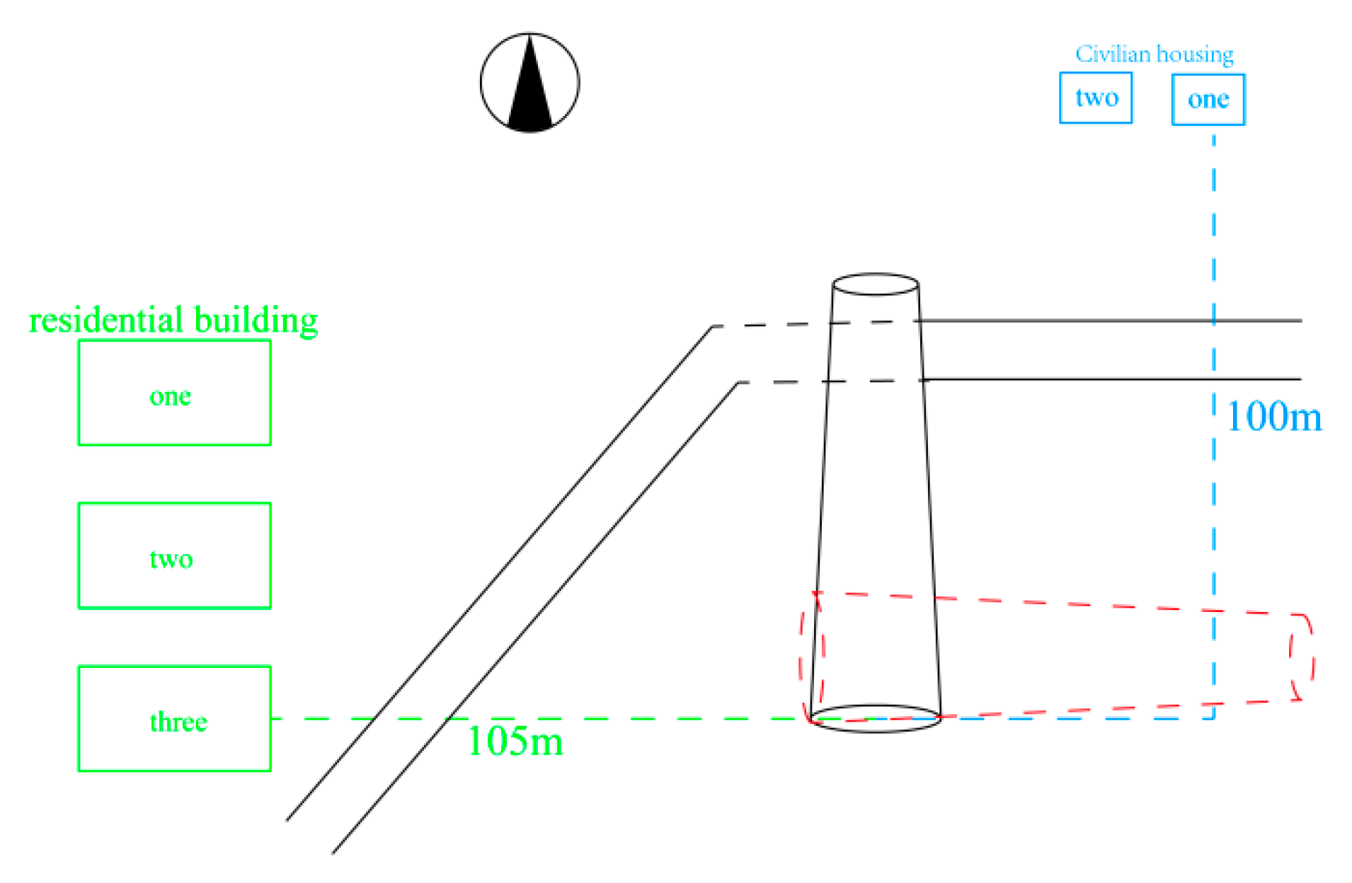
4.1. Engineering Background

This study concentrates on the demolition of abandoned chimneys in a third-tier city. The chimney in question stands at approximately 60 m tall, with a bottom outer diameter of 5.2 m and an inner diameter of roughly 3.6 m, featuring a wall thickness of 0.8 m. The surrounding environment of the chimney includes several self-built residential houses located about 100 m north of the chimney’s base, constructed with brick and concrete. Additionally, about 105 m west of the chimney’s base, there are existing residential buildings with a frame shear wall structure. Considering the chimney’s height and its surroundings, the proposed method for demolition involves blasting the base to induce a controlled collapse of the structure towards the east, as depicted in Figure 7.

4.2. Construction of the Model for Blasting Seismic Wave Signals

Per the latest iteration of the blasting safety regulations, the safe allowable vibration speed for residential buildings during blasting is set below 2 cm/s, while for reinforced concrete structural buildings, it is below 3 cm/s. This blasting project meticulously monitors the structural dynamic response of residential buildings under the influence of blasting, using the vibration velocity measured at the residential building as the primary focus of study. The TC-4850 blasting vibration meter is employed for real-time monitoring on-site, and the signals obtained undergo blasting seismic wave signal denoising processing.
We set up a monitoring station at a residential building about 100 m away from the chimney and use the TC-4850 blasting vibration to collect the generated blasting seismic waves. A typical seismic wave monitoring signal obtained from field monitoring is used as the research subject. The measured signal, as shown in Figure 8, is sampled over the interval of −0.1 to 0.6 s, with a total of 1400 data points. The period from −0.1 to 0.6 s represents the preset trigger time of the instrument.
The signal in Figure 8 is by EP-CEEMDAN-MPE decomposition, resulting in the IMFs and residual term shown in Figure 9. From Figure 9, it can be observed that the mid- and low-frequency signals are highly stable, indicating that the mid- and low-frequency characteristics of the signal are well preserved. No significant mode confusion or endpoint divergence is observed.
Based on the eight IMFs obtained from EP-CEEMDAN-MPE in Figure 9, the DM is constructed, as shown in Equation (23).
D M 1 = S t i = 1 1 I M F i D M 2 = S t i = 1 2 I M F i D M 8 = S t i = 1 8 I M F i
The S of DM1 to DM8 and the ESD between each DM and S(t) are calculated. The objective function Y is then established, and the results are presented in Table 3. The selection of the weighting coefficient β was explained in the simulated blasting vibration experiment. Here, the results for β = 0.6, β = 0.7, and β = 0.8 are directly listed.
Table 4 further demonstrates that the weighting coefficient β can control the degree of denoising to meet the requirements of practical construction. In real-world engineering applications, if preserving the original components of the signal is prioritized, β can be set to a higher value. Conversely, if significant denoising is required, β can be set to a lower value.
When β = 0.6, DM1 is optimal when only considering ESD, but its denoising effect is not significant. DM8 is optimal when only considering S, but it exhibits over-denoising. When both ESD and S are considered, DM2 is optimal. This indicates that a single metric cannot simultaneously meet the engineering requirements of effective denoising and preservation of the original signal’s authenticity. The dual-parameter optimization approach in the objective function better aligns with the needs of practical engineering construction.
Following the same analysis as for the simulated signal, a comparison plot between the DM and the original signal is generated, as shown in Figure 10. This figure further highlights the advantages of DM2, which effectively preserves the authentic information of the original signal while achieving denoising. From Figure 10, it is evident that DM6 to DM8 overly prioritize the smoothness of the model, resulting in distorted denoised signals and large error standard deviations compared to the original measured signal S(t).

4.3. Evaluation of Denoising Performance for Blasting Seismic Wave Signals

Using Matlab (R2016b) programming, the difference power PDM between S(t) and DM1 to DM8 is calculated, representing the noise power removed. Each DM’s ISNR is computed. The ISNR values for each DM are listed in Table 4. According to the properties of the logarithmic function, a larger ISNR indicates a smaller PDM, suggesting that the denoising effect is not significant.
From Table 4, it is evident that DM2 exhibits the optimal denoising performance. This result aligns with the analysis of the optimal equation solution and the DM comparison plot, demonstrating that the DM not only achieves excellent denoising results for simulated blasting vibration signals but also performs effectively in practical engineering applications for blasting seismic wave signal denoising.
Upon applying the DM to noisy seismic wave signals from actual blasting monitoring, it is observed that the model effectively denoises the signals while preserving the authentic components of the original signal. It also demonstrates strong suppression of inherent mode confusion and endpoint effects associated with EMD. This eliminates distortions in time–frequency analysis caused by noise interference, EMD mode confusion, and algorithm endpoint effects, providing robust support for the in-depth exploration of blasting seismic wave vibration characteristics and the control of blasting seismic wave hazards.

4.4. Analysis of Results

1.
Signal processing and denoising model construction occurred as follows:
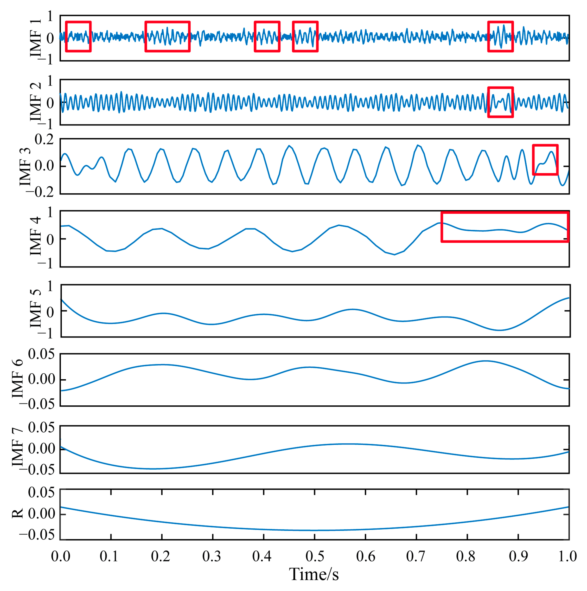
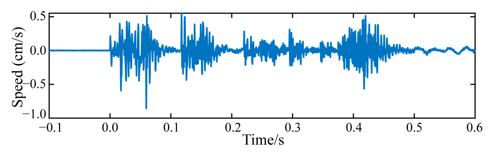
(1)
A typical seismic wave signal S(t) (Figure 8) was decomposed using EP-CEEMDAN-MPE, yielding eight IMFs and a residual term (Figure 9). The decomposition demonstrated high stability in mid- and low-frequency signals, with no significant mode confusion or endpoint divergence, validating the effectiveness of endpoint processing.
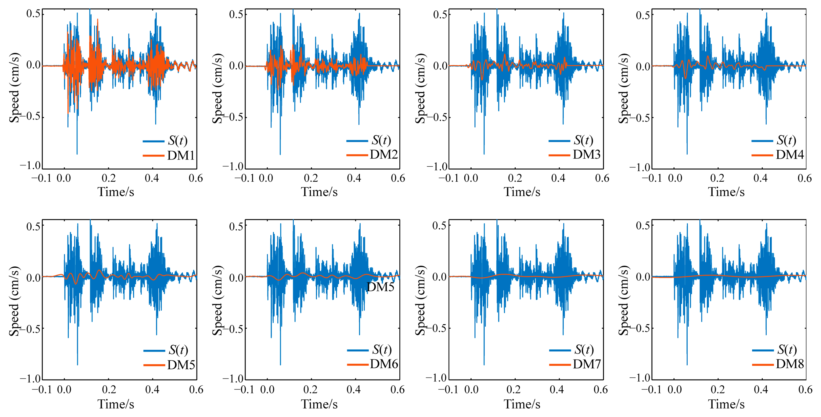
(2)
Eight denoising models (DM1 to DM8) were constructed, and their performance was evaluated using error standard deviation (ESD) and smoothness (S). The objective function Y was optimized for different weighting coefficients (β = 0.6,0.7,0.8). DM2 emerged as the optimal model, balancing denoising intensity and signal fidelity, while DM6 to DM8 exhibited over-denoising, leading to signal distortion (Table 3).
2.
Denoising performance evaluation occurred as follows:
(1)
The improved signal-to-noise ratio (ISNR) was utilized to evaluate the denoising performance. DM2 achieved the highest ISNR improvement, indicating a superior denoising capability while maintaining the authenticity of the original signal. In contrast, DM6 to DM8 resulted in negative noise reduction power, rendering ISNR calculations meaningless and emphasizing the risks of over-denoising (Table 4).
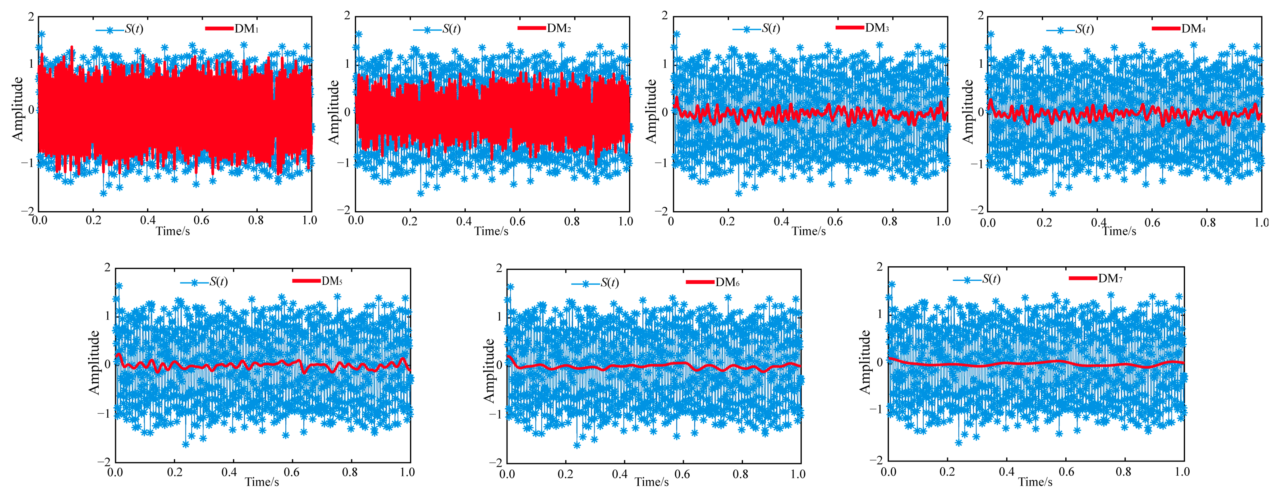
(2)
A comparison plot (Figure 10) further validated DM2’s effectiveness, demonstrating its ability to retain critical signal features while reducing noise. This aligns with the results from the simulated signal analysis, confirming the model’s consistency and reliability.

5. Discussion

This study proposes a dual denoising model for blasting seismic wave signals, addressing the critical issue of noise interference in monitoring signals, which often obscures the true characteristics of blasting vibrations. The discussion highlights the following key aspects:
(1)
Endpoint processing (EP).
The endpoint effect, a common issue in signal processing, causes signal divergence at the endpoints, especially in shorter data segments. The proposed EP method extends the signal at both ends by utilizing internal signal trends, effectively mitigating endpoint interference. This ensures the preservation of the original signal’s integrity and enhances the reliability of the denoising process.
(2)
CEEMDAN-MPE algorithm.
The CEEMDAN-MPE algorithm integrates the advantages of both CEEMDAN and MPE. CEEMDAN adaptively suppresses low-frequency noise while maintaining near-zero reconstruction error with minimal averaging iterations. MPE, employing a multi-scale coarse-graining method, controls high-frequency noise by adjusting the entropy values of the intrinsic mode functions (IMFs). This combined approach ensures that the decomposed IMFs retain clear physical significance, free from mode confusion and excessive noise.
(3)
Dual-stage denoising framework.
The initial stage of denoising employs EP-CEEMDAN-MPE to eliminate noise and mitigate endpoint effects. The subsequent phase involves constructing multiple denoising models by integrating IMFs and optimizing an objective function that harmonizes smoothness (S) with the standard deviation of reconstruction error (ESD). The optimal denoising model, selected through this process, achieves the finest equilibrium between denoising intensity and signal fidelity.
(4)
Validation with simulated signals.
The model’s performance is rigorously evaluated using simulated blasting vibration signals with a predefined signal-to-noise ratio (SNR). The results demonstrate that the model effectively reduces noise while preserving the original signal’s characteristics. The optimal denoising model, determined by minimizing the objective function, consistently outperforms other models in terms of denoising effectiveness and signal preservation.
(5)
Application to real engineering data.
The model was applied to real blasting seismic wave signals. The results confirm its practical applicability and reliability, successfully suppressing noise, mode confusion, and endpoint effects. This ensures accurate time–frequency analysis, which is crucial for understanding blasting vibration characteristics and implementing effective hazard control measures.
(6)
Scientific and practical contributions.
The proposed model tackles the limitations of current denoising techniques by integrating endpoint processing and dual-stage optimization. It offers a scientifically grounded and practical solution for denoising blasting seismic wave signals, thereby enhancing the precision of vibration analysis and hazard mitigation. This model effectively reduces noise while preserving the integrity of the original signal.
The dual denoising model introduced in this study provides a thorough and effective method to combat noise interference in blasting seismic wave signals. It rigorously confirms its noise reduction capabilities through simulations and real data noise reduction processing, and its practical application in engineering settings highlights its importance in the field of blasting vibration analysis and hazard control. Future research could investigate the model’s adaptability to various other seismic signals and its integration with real-time monitoring systems.

6. Conclusions

(1)
The denoising model significantly enhances urban controlled blasting safety by precisely extracting authentic vibration characteristics, enabling accurate hazard assessment and effective vibration control measures for the protection of critical infrastructure.
(2)
By applying endpoint processing to the blasting seismic wave monitoring signals, the interference of endpoint effects inherent in the denoising model on the evaluation of denoising performance is effectively eliminated.
(3)
The CEEMDAN-MPE algorithm, which combines the adaptability of CEEMDAN and its strong suppression capability for low-frequency noise with the robustness of MPE and its control over high-frequency noise, effectively mitigates the impact of noise on modal decomposition, yielding IMFs with clearer physical significance.
(4)
Based on the optimization principles of advanced mathematics, a denoising model is identified that enhances denoising performance while preserving the authentic components of the original monitoring signals. The denoising capability of the dual-stage denoising model is quantitatively analyzed using simulated blasting vibration signals with a specified signal-to-noise ratio (SNR).
(5)
The denoising results for both the simulated signals with a specified signal-to-noise ratio (SNR) and the actual engineering blasting seismic wave signals are consistent, demonstrating the reliability and effectiveness of the denoising model in noise reduction applications.

Author Contributions

Conceptualization, M.S. and J.W.; methodology, M.S. and H.Z.; software, M.S. and J.W.; validation, M.S. and Y.L.; data curation, M.S. and L.W.; writing—original draft preparation, M.S.; writing—review and editing, M.S. and J.Y.; funding acquisition, L.W., M.S. and J.W. All authors have read and agreed to the published version of the manuscript.

Funding

This research was funded by the National Natural Science Foundation of China, 41907259; and the foundation of Research Center of Hubei Small Town Development, 2024A004; the Natural Science Foundation of Hubei Province of China, 2022CFB948; and the Foundation of Engineering Research Center of Rock-Soil Drilling & Excavation and Protection, 202404 and 202409.

Data Availability Statement

Data is contained within the article.

Conflicts of Interest

The authors declare no conflicts of interest.

Nomenclature

S(t)Signal
S(t)iThe i-th part of the signal
MDMatching degree
dDistances
rCorrelation coefficient
ysjMulti-scale time series
Bj(t)The adaptive white noise
αjThe standard deviation of the j-th white noise
IMFiIntrinsic mode function
R(t)The remainder
DMDenoising model
βThe weighting coefficient
ESDThe error standard deviation
f(x); u(x); v(x)The smooth curve
u-(w0)The left limit of u(x) at w0
v+ (w0)The right limit of v(x) at w0
Ku|w=w0The curvatures of u(x)
Kv|w=w0The curvatures of v(x)
u’’(w0)The second derivatives of u(x) at w0
v’’(w0)The second derivatives of v(x) at w0
SThe smoothness
YThe objective function
NThe total number of sampling points
x0Any arbitrary point within N
hThe sampling interval
SNRSignal-to-noise ratio
PnThe effective power of the noise
PsThe effective power of the signal
x(t)A noise-free signal
n(t)A noise signal
ISNRImproved signal-to-noise ratio
PDMThe power of the denoising model

References

  1. Zhao, Z.Y.; Zhang, Y.; Bao, H.R. Tunnel blasting simulations by the discontinuous deformation analysis. Int. J. Comput. Methods 2011, 8, 277–292. [Google Scholar] [CrossRef]
  2. Meng, X.Z.; Wang, Z.S.; Zhang, Z.Z.; Wang, F.Q. A Method for Monitoring the Underground Mining Position Based on the Blasting Source Location. Meas. Sci. Rev. 2013, 13, 45–49. [Google Scholar] [CrossRef]
  3. Abbaszadeh Shahri, A.; Pashamohammadi, F.; Asheghi, R.; Abbaszadeh Shahri, H. Automated intelligent hybrid computing schemes to predict blasting induced ground vibration. Eng. Comput. 2021, 38, 3335–3349. [Google Scholar] [CrossRef]
  4. Huang, Y.; Zhou, Z.; Li, M.; Luo, X. Prediction of Ground Vibration Induced by Rock Blasting Based on Optimized Support Vector Regression Models. Comput. Model. Eng. Sci. 2024, 139, 3147–3165. [Google Scholar] [CrossRef]
  5. Huang, W.X.; Liu, D.W. Mine microseismic signal denosing based on variational mode decomposition and independent component analysis. J. Vib. Shock 2019, 38, 56–63. (In Chinese) [Google Scholar]
  6. Liu, J.C.; Gao, W.X. Vibration Signal Analysis of Water Seal Blasting Based on Wavelet Threshold Denoising and HHT Transformation. Adv. Civ. Eng. 2020, 2020, 4381480. [Google Scholar] [CrossRef]
  7. Zhao, M.S.; Zhang, J.H.; Yi, C.P. Time-frequency characteristics of blasting vibration signals measured in milliseconds. Min. Sci. Technol. 2011, 21, 349–352. (In Chinese) [Google Scholar] [CrossRef]
  8. Li, X.; Li, Z.; Wang, E.; Feng, J.; Chen, L.; Li, N.; Kong, X. Extraction of microseismic waveforms characteristics prior to rock burst using Hilbert—Huang transform. Measurement 2016, 2016, 101–113. [Google Scholar] [CrossRef]
  9. Yuan, H.; Liu, X.; Liu, Y.; Bian, H.; Chen, W.; Wang, Y. Analysis of Acoustic Wave Frequency Spectrum Characters of Rock Mass under Blasting Damage Based on the HHT Method. Adv. Civ. Eng. 2018, 2018, 9207476. [Google Scholar] [CrossRef]
  10. Wu, Z.; Huang, N.E. A study of the characteristics of white noise using the empirical mode decomposition method. Proc. Math. Phys. Eng. Sci. 2004, 460, 1597–1611. [Google Scholar] [CrossRef]
  11. Zheng, J.D.; Chen, J.S.; Yang, Y. Modified EEMD algorithm and its applications. J. Vib. Shock 2013, 32, 21–26. (In Chinese) [Google Scholar] [CrossRef]
  12. Gaci, S. A New Ensemble Empirical Mode Decomposition (EEMD) Denoising Method for Seismic Signals. Energy Procedia 2016, 97, 84–91. [Google Scholar] [CrossRef]
  13. Cheng, J.S.; Wang, J.; Gui, L. An improved EEMD method and its application in rolling bearing fault diagnosis. J. Vib. Shock 2018, 37, 51–56. (In Chinese) [Google Scholar] [CrossRef]
  14. Sun, M.; Wu, L.; Yang, J.K. Application research on time-frequency analysis of underground tunnel blasting vibration based on CEEMDAN-INHT. Blasting 2024, 41, 14–20. Available online: https://www.sciopen.com/article/10.3963/j.issn.1001-487X.2024.01.003 (accessed on 25 April 2025). (In Chinese).
  15. Ditommaso, R.; Mucciarelli, M.; Parolai, S.; Picozzi, M. Monitoring the structural dynamic response of a masonry tower: Comparing classical and time-frequency analyses. Bull. Earthq. Eng. 2012, 10, 1221–1235. [Google Scholar] [CrossRef]
  16. Zhong, G.S.; Xu, G.Y.; Jiang, W.W. Application of de-noising in blasting seismic signals based on wavelet transform. J. Cent. South Univ. 2006, 37, 155–159. [Google Scholar]
  17. Beenamol, M.; Prabavathy, S.; Mohanalin, J. Wavelet based seismic signal de-noising using Shannon and Tsallis entropy. Comput. Math. Appl. 2012, 64, 3580–3593. [Google Scholar] [CrossRef]
  18. Srivardhan, V. Stratigraphic correlation of wells using discrete wavelet transform with fourier transform and multi-scale analysis. Geomech. Geophys. Geo-Energy Geo-Resour. 2016, 2, 137–150. [Google Scholar] [CrossRef]
  19. Huang, N.E. New method for nonlinear and nonstationary time series analysis: Empirical mode decomposition and Hilbert spectral analysis. Proc. SPIE—Int. Soc. Opt. Eng. 2000, 4056, 197–209. [Google Scholar] [CrossRef]
  20. Ditommaso, R.; Mucciarelli, M.; Ponzo, F. Analysis of non-stationary structural systems by using a band-variable filte. Bull. Earthq. Eng. 2012, 2012, 10. [Google Scholar] [CrossRef]
  21. Li, X.; Wang, E.; Li, Z.; Bie, X.; Chen, L.; Feng, J.; Li, N. Blasting wave pattern recognition based on Hilbert-Huang transform. Geomech. Eng. 2016, 11, 607–624. [Google Scholar] [CrossRef]
  22. Huang, N.E.; Shen, Z.; Long, S.R.; Wu, M.C.; Shih, H.H.; Zheng, Q.; Yen, N.C.; Tung, C.C.; Liu, H.H. The empirical mode decomposition and the Hilbert spectrum for nonlinear and non-stationary time series analysis. Proc. R. Soc. A 1998, 454, 903–995. [Google Scholar] [CrossRef]
  23. Huang, N.E.; Shen, Z.; Long, S.R. A new view of nonlinear water waves: The Hilbert spectrum. Annu. Rev. Fluid Mech. 1999, 31, 417–457. [Google Scholar] [CrossRef]
  24. Vashishtha, G.; Kumar, R. Autocorrelation energy and aquila optimizer for MED filtering of sound signal to detect bearing defect in Francis turbine. Meas. Sci. Technol. 2022, 33, 015006. [Google Scholar] [CrossRef]
  25. Yeh, J.R.; Shieh, J.S.; Huang, N.E. Complementary Ensemble Empirical Mode Decomposition: A Novel Noise Enhanced Data Analysis Method. Adv. Adapt. Data Anal. 2010, 2, 135–156. [Google Scholar] [CrossRef]
  26. Wu, Z.; Huang, N.E. Ensemble empirical mode decomposition: A noise-assisted data analysis method. Adv. Adapt. Data Anal. 2011, 1, 1–41. [Google Scholar] [CrossRef]
  27. Zhou, Y.; Li, H. Adaptive noise reduction method for DSPI fringes based on bi-dimensional ensemble empirical mode decomposition. Opt. Express 2011, 19, 18207–18215. [Google Scholar] [CrossRef]
  28. Zhang, J.; Jin, Y.; Sun, B.; Han, Y.; Hong, Y. Study on the Improvement of the Application of Complete Ensemble Empirical Mode Decomposition with Adaptive Noise in Hydrology Based on RBFNN Data Extension Technology. Comput. Model. Eng. Sci. 2021, 126, 755–770. [Google Scholar] [CrossRef]
  29. Peng, Y.X.; Liu, Y.S.; Zhang, C.; Wu, L. A Novel Denoising Model of Underwater Drilling and Blasting Vibration Signal Based on CEEMDAN. Arab. J. Sci. Eng. 2021, 46, 4857–4865. [Google Scholar] [CrossRef]
  30. Wang, Y.S.; Ma, Q.H.; Zhu, Q.; Liu, X.T.; Zhao, L.H. An intelligent approach for engine fault diagnosis based on Hilbert-Huang transform and support vector machine. Appl. Acoust. 2014, 1, 1–9. [Google Scholar] [CrossRef]
  31. Jiao, Y.X.; Li, K.Z.; Yue, Z.; Ban, H.F.; Liang, L.F.; Tian, C.D.; Shen, Y.Y. CEEMDAN combined wavelet denoising improved the MW cycle slip detection algorithm. Sci. Rep. 2025, 14, 23487. [Google Scholar] [CrossRef] [PubMed]
  32. Li, P.; Lu, W.B.; Qiao, X.M.; Chen, M.; Yan, P. Signal processing and response analysis of blasting vibration induced by high rock slope excavation. J. China Coal Soc. 2011, 39, 401–405. (In Chinese) [Google Scholar]
  33. Zhao, Y.; Shan, R.L.; Wang, H.L.; Tong, X.; Li, Y.H. Regression analysis of the blasting vibration effect in cross tunnels. Arab. J. Geosci. 2021, 14, 1925. [Google Scholar] [CrossRef]
  34. Lou, J.W.; Long, Y. Research on Feature Extraction and Recognition Technology of Blasting Vibration Signal. Vib. Shock 2003, 22, 4. [Google Scholar]
  35. Yuan, H.P.; Zou, Y.Y.; Li, H.Z.; Ji, S.J.; Gu, Z.A.; He, L.; Hu, R.C. Assessment of peak particle velocity of blast vibration using hybrid soft computing approaches. J. Comput. Des. Eng. 2025, 12, 154–176. [Google Scholar] [CrossRef]
  36. Torres, M.E.; Colominas, M.A.; Schlotthauer, G.; Flandrin, P. A complete ensemble empirical mode decomposition with adaptive noise. In Proceedings of the 2011 IEEE International Conference on Acoustics, Speech, and Signal Processing, ICASSP, Prague, Czech Republic, 22–27 May 2011; pp. 4143–4147. [Google Scholar] [CrossRef]
  37. Yao, W.P.; Liu, T.B.; Dai, J.F.; Wang, J. Multiscale permutation entropy analysis of electroencephalogram. Acta Phys. Sin. 2014, 63, 427–433. [Google Scholar] [CrossRef]
  38. Chen, S.J.; Shang, P.J.; Wu, Y. Multivariate multiscale fractional order weighted permutation entropy of nonlinear time series. Phys. A: Stat. Mech. Its Appl. 2019, 515, 217–231. [Google Scholar] [CrossRef]
  39. Zhang, Y.Y.; Yang, Z.X.; Du, X.L.; Luo, X.Y. A New Method for Denoising Underwater Acoustic Signals Based on EEMD, Correlation Coefficient, Permutation Entropy, and Wavelet Threshold Denoising. J. Mar. Sci. Appl. 2024, 23, 222–237. [Google Scholar] [CrossRef]
  40. Li, J.; Li, Q. Medium term electricity load forecasting based on CEEMDAN-permutation entropy and ESN with leaky integrator neurons. Electr. Mach. Control. 2015, 19, 70–80. (In Chinese) [Google Scholar] [CrossRef]
Figure 1. EP-CEEMDAN-MPE algorithm flow chart.
Buildings 15 01751 g001
Figure 2. Second stage of denoising: optimal function solution flow chart.
Buildings 15 01751 g002
Figure 3. Simulation signal and its composition signal.
Buildings 15 01751 g003
Figure 4. The first-stage denoising process of the simulated signals: IMF obtained by EP-CEEMDAN-MPE algorithm.
Buildings 15 01751 g004
Figure 5. IMF obtained by CEEMDAN-MPE algorithm.
Buildings 15 01751 g005
Figure 6. Comparison diagram of DM and S(t).
Buildings 15 01751 g006
Figure 7. Environmental map around directional blasting chimney.
Buildings 15 01751 g007
Figure 8. Measured seismic wave monitoring signal S(t).
Buildings 15 01751 g008
Figure 9. The first-stage denoising process of the measured signal S(t): IMF obtained by EP-CEEMDAN-MPE algorithm.
Buildings 15 01751 g009
Figure 10. Comparison diagram of DM.
Buildings 15 01751 g010
Table 1. ESD, S, and Y values of simulated signal denoising models.
DMESDSY
β = 0.6β = 0.7β = 0.8β = 0.8845
DM10.06281.00000.43770.34400.25020.1710
DM20.17620.13030.15780.16240.16700.1709
DM30.41870.00880.25470.29570.33670.3714
DM40.53970.00110.32430.37810.43200.4775
DM50.91540.00020.54930.64080.73240.8097
DM60.96370.000020.57820.67460.77100.8524
DM71.00001.1361 × 10−70.60000.70000.80000.8845
Note: ESD, S, and Y in Table 1 are all linearly standardized data and dimensionless.
Table 2. Correlation parameters based on given signal-to-noise ratio.
DMSNRISNRISNR-SNR
DM11012.87582.8758
DM217.24807.2480
DM310.09140.0914
DM4(PDM-Pn) < 0, Logarithmically meaningless(PDM-Pn) < 0, Logarithmically meaningless
DM5(PDM-Pn) < 0, Logarithmically meaningless(PDM-Pn) < 0, Logarithmically meaningless
DM6(PDM-Pn) < 0, Logarithmically meaningless(PDM-Pn) < 0, Logarithmically meaningless
DM7(PDM-Pn) < 0, Logarithmically meaningless(PDM-Pn) < 0, Logarithmically meaningless
Table 3. ESD, S, and Y of each DM.
DMESDSY(β = 0.6)Y(β = 0.7)Y(β = 0.8)
DM10.06281.00000.43770.34400.2502
DM20.17620.13030.15780.16240.1670
DM30.41870.00880.25470.29570.3367
DM40.53970.00110.32430.37810.4320
DM50.91540.00020.54930.64080.7324
DM60.96370.000020.57820.67460.7710
DM70.99918.7264 × 10−70.59950.69940.7993
DM81.00001.1361 × 10−70.60000.70000.8000
Note: ESD, S, and Y in Table 1 are all linearly standardized data and dimensionless.
Table 4. Measured signal related parameters.
DMPsPDMISNR
DM11.3874 × 10−21.2476 × 10−22.3321
DM21.3782 × 10−20.0289
DM31.3365 × 10−20.2938
DM41.3277 × 10−20.1910
DM51.3146 × 10−20.2341
DM61.3032 × 10−20.2719
DM71.2904 × 10−20.3148
DM81.2774 × 10−20.3587
Disclaimer/Publisher’s Note: The statements, opinions and data contained in all publications are solely those of the individual author(s) and contributor(s) and not of MDPI and/or the editor(s). MDPI and/or the editor(s) disclaim responsibility for any injury to people or property resulting from any ideas, methods, instructions or products referred to in the content.

