Exploring the Joint Influence of Built Environment Factors on Urban Rail Transit Peak-Hour Ridership Using DeepSeek

Abstract

Modern cities are facing increasing challenges such as traffic congestion, high energy consumption, and poor air quality, making rail transit systems, known for their high capacity and low emissions, essential components of sustainable urban infrastructure. While numerous studies have examined how the built environment impacts transit ridership, the complex interactions among these factors warrant further investigation. Recent advancements in the reasoning capabilities of large language models (LLMs) offer a robust methodological foundation for analyzing the complex joint influence of multiple built environment factors. LLMs not only can comprehend the physical meaning of variables but also exhibit strong non-linear modeling and logical reasoning capabilities. This study introduces an LLM-based framework to examine how built environment factors and station characteristics shape the transit ridership dynamics by utilizing DeepSeek-R1. We develop a 4D + N variable system for a more nuanced description of the built environment of the station area which includes density, diversity, design, destination accessibility, and station characteristics, leveraging multi-source data such as points of interest (POIs), road network data, housing prices, and population data. Then, the proposed approach is validated using data from Qingdao, China, examining both single-factor and multi-factor effects on transit peak-hour ridership at the macro level (across all stations) and the meso level (specific station types). First, the variables that have a substantial effect on peak-hour transit ridership at both the macro and meso levels are discussed. Second, key and latent factor combinations are identified. Notably, some factors may appear to have limited importance at the macro level, yet they can substantially influence the peak-hour ridership when interacting with other factors. Our findings enable policymakers to formulate a balanced mix of soft and hard policies, such as integrating a flexitime policy with enhancements in active travel infrastructure to increase the attractiveness of public transit. The proposed analytical framework is adaptable across regions and applicable to various transportation modes. These insights can guide transportation managers and policymakers while optimizing Transit-Oriented Development (TOD) strategies to enhance the sustainability of the entire transportation system.

1. Introduction

To reduce traffic congestion in metropolitan areas, the significance of facilitating public transport use has been highlighted in recent decades. Mass transit systems, including bus rapid transit (BRT) and urban rail transit (URT), have become a central pillar of urban public transport owing to their high capacity and efficiency. Rail transit in China is experiencing strong growth. By the end of 2024, there are 325 metro lines in service in 54 cities, with an operating mileage of 10,945.6 km [1]. However, urban rail transit’s trip-sharing rate remains relatively low (30.83%) [2]. In many cities, public transit struggles to attract users due to issues such as service unreliability and localized overcrowding at peak times caused by unbalanced spatial and temporal ridership distributions. Identifying the factors that influence these ridership fluctuations is therefore crucial. This knowledge forms the foundation for optimizing both public transport planning and integrated land use strategies, such as Transit-Oriented Development (TOD), ultimately improving the operational management of public transport and encouraging residents to choose public transit over other travel modes.

Extensive studies have investigated the relationship between transit ridership and its influencing factors, indicating that the interaction of built environment characteristics, such as population density, land use, socioeconomic factors, and traffic accessibility, strongly influences transit ridership. The classical four-step model (FSM)—comprising trip generation, trip distribution, mode choice, and traffic assignment—is commonly adopted in estimating transit demand [3,4]. However, this approach is more suitable for forecasting transit ridership at the macroscopic or regional scale rather than at the microscopic or station-level scale [4,5]. It also has some practical downsides, such as insensitivity to land use and high implementation costs [6]. Recently, the direct ridership model (DRM), as an alternative to the FSM, has been spotlighted for exploring the factors that affect transit ridership via regression methods. DRMs are widely preferred for their cost-effectiveness, methodological simplicity, interpretability, computational efficiency, and rapid responsiveness in comparison to FSMs [7]. A great many empirical studies have been conducted using DRMs in many major cities worldwide [8,9,10,11].

With the increasing complexity of modern urban development, the availability of multi-source data, and advancements in artificial intelligence technology, the research paradigm for understanding the relationships between built environment factors and transit ridership has undergone a significant transformation. The scale of built environment measurements has gradually shifted from the previously dominant macro scale to the meso and micro scales. In the 1990s, Cervero and Kockelman [12] proposed the 3Ds framework (density, diversity, design): density reflects the concentration of the population, buildings, or facilities in an area, commonly measured through indicators such as the population density, point of interest (POI) density, floor area ratio (FAR), etc.; diversity emphasizes the degree of mixed land use, such as the balanced distribution of residential, commercial, and public service land, typically measured through the land use mix; design focuses on street network connectivity and spatial morphology, including the intersection density, road density, and walkability. To address the limitations of the 3Ds framework, Ewing and Cervero [13] added two additional dimensions—destination accessibility and distance to transit—forming the 5Ds model, which reflects an increased emphasis on commuting efficiency and non-motorized travel. In recent years, some scholars have attempted to characterize the built environment using a more refined 7Ds indicator system, adding demand management and demographics dimensions to the 5Ds framework [14]. Regarding the research methodologies, early studies predominantly assumed linear relationships between the built environment and travel behavior, employing linear regression models (e.g., ordinary least squares (OLS) regression, two-stage least squares (2SLS) regression) [8,15]. As the 5Ds model incorporated more factors, multicollinearity issues emerged among many variables. An et al. applied a principal component analysis reducing the dimensionality of POI data and used the resulting groups of POIs as independent variables in an OLS regression model [16]. However, linear regression also overlooks spatial heterogeneity, prompting researchers to propose geographically weighted regression (GWR) and its improved variants to address this issue [5,17,18,19,20,21,22]. Nevertheless, these models remain essentially linear, while built environment factors typically exhibit complex, non-linear relationships. Ding et al. pioneered the use of gradient boosting decision tree (GBDT) to analyze the non-linear effects of built environment factors on transit ridership [23]. Subsequently, other scholars have employed various machine learning techniques such as Light Gradient Boosting Machine (LightGBM), back propagation neural networks (BPNNs), and Long Short-Term Memory (LSTM) networks to enrich the related findings [24,25,26].

This paradigm shift in the research approaches presents several challenges for the methodology. While machine learning models can capture the non-linear effects of built environment factors better, they inherently struggle with two major methodological constraints: (1) a profound inability to comprehend the physical significance of built environment indicators, rendering the models “black boxes”, and (2) the high dimensionality and multicollinearity among built environment indicators, which substantially increases the complexity of modeling and undermines the interpretability of the results.

With the emergence of reasoning-oriented large language models such as OpenAI’s o1 and DeepSeek-R1, a new research paradigm has been introduced into this field. These models not only comprehend the physical significance of built environment indicators but also possess advanced numerical reasoning and logical chain inference capabilities. For instance, DeepSeek-R1 achieved a score of 92.1 on the MATH-500 benchmark, significantly surpassing GPT-4 and Claude 3.5 [27]. The reasoning capabilities of LLMs in this study are primarily manifested in three dimensions: first, pattern recognition, which captures complex dependencies between variables via a self-attention mechanism; second, symbol grounding, which maps numerical data to semantic spaces (e.g., high store counts correspond to commercially active areas); third, generative reasoning, which generates counterfactual scenarios based on the historical data distribution (e.g., how would ridership change if store counts increase by 10?). These capabilities enable LLMs to quantify the interactions between the built environment and station characteristic factors, as well as their joint influences on transit ridership. Furthermore, by integrating domain knowledge, LLMs can analyze the results to uncover underlying mechanisms and derive actionable policy implications. Hence, to address the aforementioned challenges, this paper proposed a transit ridership interpretation framework based on DeepSeek-R1, a reasoning-oriented large language model, and presented a case study using data from Qingdao, China. Automatic fare collection (AFC) data were used to extract transit ridership. Multi-source data, including POI data from Baidu Map, road network data from Open Street Map (OSM), high-resolution remote sensing images from Tianditu, and housing price data from Lianjia.com, were integrated to conduct precise measurements of the built environments of station areas. Leveraging the LLM’s understanding and reasoning capabilities regarding the features of the built environment, we analyzed both the single-factor and multi-factor influences on the station-level transit ridership during weekday peak hours. Furthermore, we compared our predictions with those from the classical AutoRegressive Integrated Moving Average (ARIMA) and eXtreme Gradient Boosting (XGBoost) models, thereby substantiating the reliability of our LLM-based approach.

The merits of this paper are twofold:

• We propose a DeepSeek-based analytical framework that employs a chain-of-thought prompting strategy, where each stage is executed and validated independently before proceeding to the next. This iterative interaction ensures reliability, minimizes AI hallucinations, and enhances the model’s interpretability. Furthermore, the framework is adaptable and could be extended to studies in other regions, different transportation modes, and even multimodal public transit systems.
• Utilizing open-source data—including POIs, road network data, remote sensing imagery, and subway station characteristics—we construct 4Ds + N (density, diversity, design, destination accessibility, station characteristics) metrics. Using both univariate and multivariate analyses conducted at the macro (network level) and meso–micro (station-level) scales, our study identified key individual factors as well as significant factor combinations that influence transit ridership. Notably, certain factors with low single-factor importance demonstrated a substantial influence on ridership when interacting with other variables. These findings provide a reference for rail transit operators and policymakers, who can expand the framework further with additional data to obtain more enriched results, ultimately offering guidance for TOD planning and decision-making.

The remainder of this paper is structured as follows: In Section 2, we review related studies on the correlations between the built environment and transit ridership. Section 3 describes the study area, data collection, and variables in this study. Section 4 explains the methodology in detail, including the DeepSeek-based analytical framework, prompt construction, and evaluation metrics. The analytical results and their implications for our case study are presented in Section 5. We conclude this paper and suggest directions for future work in Section 6.

2. Related Work

Previous studies have demonstrated that transit ridership is the key data foundation for both transportation and urban planning. Depending on different scenarios, ridership generally contains two categories: station ridership (the boarding/alighting per station) and station-to-station ridership (the passenger flow between pairs of stations). Many studies have developed regression models for weekday [8,10], morning, and evening peak hours [28,29,30] and boarding and alighting [31,32] ridership separately to investigate the influence of the determined variables on ridership further. On the other hand, some researchers have adopted station-to-station ridership as a dependent variable to explore the impact of origin and destination factors [28,29,33]. In either case, transit ridership is influenced by a series of external factors (land use, socioeconomic characteristics), internal factors (transit network, service level, station type), and intermodal connections (feeder buses, the availability of parking), as well as various other factors. Since the objective of this study is to explore how built environment factors in station areas affect rail transit ridership, our review mainly focuses on two aspects: on the one hand, the various dimensions from which the existing research constructs built environment indicators, and on the other hand, the methodologies employed in the existing research to study the impact of the built environment on ridership.

2.1. Built Environment Factors and Station Characteristics

The development and optimization of URT systems require an in-depth understanding of various factors influencing ridership. Transit ridership analyses are typically conducted at the station level, with the built environment characteristics of station areas playing a crucial role in shaping transit ridership. A review of the relevant literature from recent decades reveals that the built environment around the station has a significant impact on transit ridership [8,9,10,34,35,36].

Regarding the measurement of built environment features, scholars have generally followed the 3Ds framework proposed by Cervero and Kockelman when constructing indicators [12]. This framework was later expanded by Ewing and Cervero into the 5Ds, which represent density, diversity, design, destination accessibility, and distance to transit [13]. Since “distance to transit” does not apply to transit ridership studies, we reviewed the factors adopted in the relevant research for the other 4Ds. Density: Population and employment density in station areas have been found to be significantly and positively associated with transit ridership, both in the developed [37] and developing world [29]. The proportions of different land use properties (e.g., commercial, residential, administrative, and recreational land) have commonly been employed as land use variables [10,25,28,32]. Various categories of POI density have also been utilized to provide a more detailed description of the land use characteristics [16,17,22,24,38]. Diversity: Some studies have measured land use diversity using “land use mix index” as a key explanatory variable, and the findings are mixed in different empirical studies. Gutierrez et al. [6] and Jun et al. [19] found that the index has a positive impact on ridership. In contrast, some studies [5,34,37,39] reported that land use mix index was not a significant factor. Ding et al. [23] further indicated that the index becomes effective only when its value exceeds 0.5. Design: The street network characteristics, such as road density and intersection density, were also mentioned in some studies. Zhao et al. [29] found that road density has a significantly positive impact on transit ridership. As for intersection density, Durning et al. [37] found that it has positively impacted ridership in Canada’s five largest cities. Inversely, Jun et al. [19] observed a negative impact of intersection density on metro ridership in Seoul. Destination accessibility: The distance to the city center, as a measure of regional accessibility, is also mentioned in some studies. Zhao et al. [29] found that the effect of the distance to the city center on station-level transit ridership was insignificant in Nanjing, China. Meanwhile, Liu et al. [34] observed a negative impact of distance to the city center on metro ridership in Washington, US. Except for built environment factors, the internal factors of the rail transit system have also been mentioned in some studies, such as station type [8,23,29] and transit service quality [34,40,41].

2.2. Approaches to Modeling Transit Ridership

In the majority of previous studies on the impact of land use on transit ridership, conventional econometric models, such as OLS regression [8,9,10,16,34,42], 2SLS regression [15,36], and Poisson regression [28], have commonly been employed. Kuby et al. [8], Loo et al. [9], Zhao et al. [10], Pan et al. [11], He et al. [42], and An et al. [16] exploited multiple linear regression to model ridership at the station level, while Choi et al. [28], Zhao et al. [29], and Kepaptsoglou et al. [40] developed multiplicative models which assumed that ridership was related to the product of the explanatory variables. This kind of direct demand model is straightforward and explainable, but there is a problem that cannot be neglected, which is that the ridership for each station is assumed to be independent (the spatial homogeneity hypothesis). In truth, there are spatial dependence and spatial heterogeneity from place to place. To capture the spatial effects on transit ridership, geographically weighted regression (GWR) [5,17,18], distance-decay regression [6], and network kriging regression [35] methods have been adopted in recent studies. The GWR model is an extended form of ordinary linear regression in space, which embeds the geographic location of the observation data into the regression coefficients and allows local independent regression for each observation point. Some improved GWR models have also been developed in recent studies [19,20,21,22]. Recently, with artificial intelligence becoming gradually more popular, machine learning methods, such as cluster analysis [43], gradient boosting decision tree (GBDT) [23,44,45], Light Gradient Boosting Machine (LightGBM) [24], and back propagation neural network (BPNN) [25], have been employed to explore the potential non-linear impact of the characteristics of the built environment on rail transit ridership.

By examining scholars’ continual exploration of the built environment’s impact on transit ridership, we have summarized a paradigm shift in the study of built environment factors. Driven by the complexity of urban development and enriched by increasingly available data, the indicator system for the built environment has continuously expanded from 3Ds to 5Ds and then to experimental 7Ds frameworks [14]. The research scale has progressively advanced from the initial macro level to the meso–micro levels. The research methods have also gradually transitioned from linear models to non-linear models. However, as the characterization of built environment indicators becomes increasingly refined, the high degree of overlap between indicators significantly increases the modeling complexity. Furthermore, there is limited literature thoroughly examining the joint influence of various built environment factors on transit ridership.

3. The Study Area and Data Collection

3.1. The Study Area

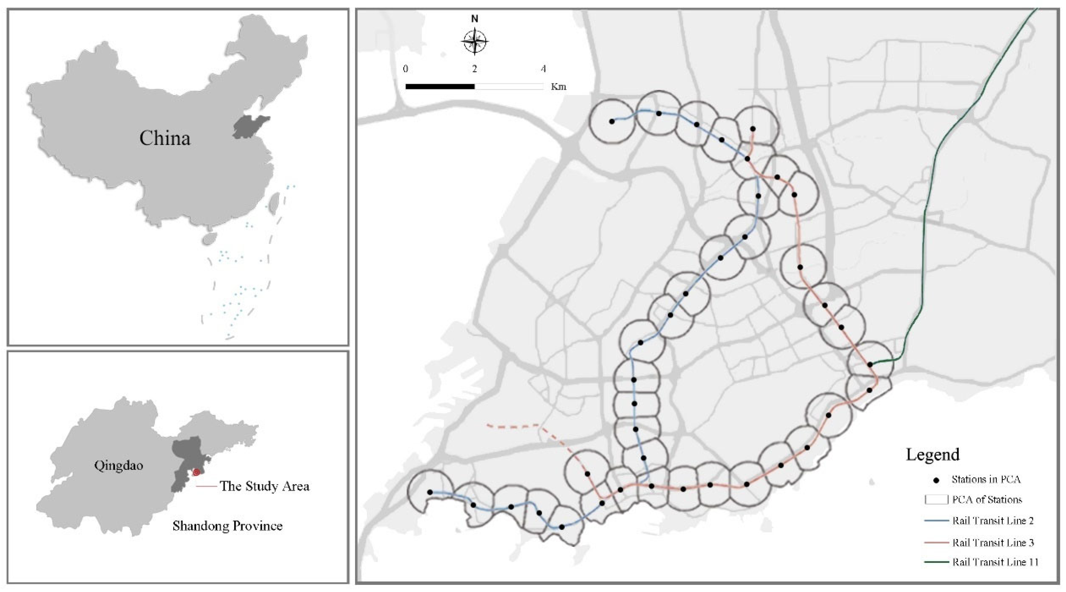
In this study, we focused on the city of Qingdao in Shandong province. Located in East China, Qingdao is the economic center of Shandong province, an international seaport city and tourist city. As one of China’s 14 megacities (with a resident population of 10.07 million in the 2020 census) [46], it faces escalating challenges due to population growth: motor vehicle ownership surged to 3.99 million units by 2023 (annual growth of 3.1%), driving rising traffic congestion and emissions [47]. The transit sharing rate is about 43%, and the daily average ridership is about 1.5 million. Qingdao metro currently has eight lines in operation, while nine are under construction, and its operating mileage will soon exceed 500 km [48].

The smart card data (SCD) used in this study were provided by the Qingdao Municipal Commission of Transport and date from July 2018. At that time, three metro lines were in operation in Qingdao: Line 2, Line 3, and Line 11. Among them, Line 11 is an inter-city transit line, while Lines 2 and 3 serve the inner city, connecting two major railway stations and several commercial areas. These two lines form the backbone of Qingdao’s metro network. Therefore, our study covers Lines 2 and 3, which contains 38 metro stations (including 3 transfer stations).

To quantify the built environment factors around the metro stations, we applied the Pedestrian Catchment Area (PCA) as a metric range. As ascertained by reviewing previous studies, researchers usually set the station service radius between 400 and 800 m [16,23,28,29,33]. Following the “Guidelines for planning and design of areas along Urban Rail Transit” proposed by the Ministry of Housing and Urban-Rural Development of China, an area about 300–500 m away from the station is suggested as the core impact area, and an area 500 to 800 m away from the station, within an approximately fifteen-minute walk to the station’s entrance, is defined as the rail transit impact area. By considering the metro station spacing in Qingdao and the overlaps between adjacent PCAs, this study sets the radius of the PCA to 600 m to quantify the built environment of the station areas better. The overlapping parts of the PCAs are segmented by Thiessen polygons in ArcGIS (Version 10.6). It should be noted that there are ten coastal stations whose PCAs contain sea areas, which affects the subsequent calculation of certain indicators (e.g., road density, population density) within the PCA; hence, we used ArcGIS to remove invalid sea areas from each PCA to obtain the final PCAs for Line 2 and Line 3 of Qingdao metro, which are shown in Figure 1.

3.2. Smart Card Data (SCD)

We acquired one month of SCD from Qingdao metro during July of 2018, with a total number of trip records of over fourteen million. The SCD records were obtained from the automatic fare collection (AFC) system of Qingdao metro and contained all trips paid for using one-way tickets and registered and anonymous public transport cards. Each record includes a card number, transaction date, transaction time, transaction type (tap-in or tap-out), and station code. Accordingly, the boarding and alighting ridership at each station can be counted by the time of day. Through preprocessing, we ultimately obtained the number of boarding and alighting passengers at each station during morning and evening peak hours, which served as dependent variables for our modeling and further analysis.

3.3. Open-Source Data

This study employed five kinds of open-source data, including POIs extracted from Baidu Map (a leading Chinese digital mapping platform, ensuring comprehensive representation of urban functions), housing price data from Lianjia.com (a major Chinese real estate platform with verified transaction records), road network data from OpenStreetMap (OSM), high-definition remote sensing images from Tianditu (China’s national geospatial information public service platform, offering authoritative and high-resolution satellite imagery for land use classification), and population data from WorldPop.

The POIs from Baidu Map were obtained in 2018, which matched the time of the SCD. All of the POIs include a name, address, longitude and latitude (Baidu Map uses the BD09 encrypted coordinate system. When importing POIs into ArcGIS, we first convert BD09 coordinates into GCJ02 coordinates using Baidu’s provided offset algorithm, followed by converting the GCJ02 coordinates into WGS84 using a reverse engineering algorithm.), and classification. Various categories of POIs can represent specific types of land use, which in turn determine travel demands. Nevertheless, the original classification from Baidu Map is not completely appropriate for analyzing public transit demands, and a few categories of POIs needed to be re-classified or even removed. For instance, automobile services (e.g., petrol stations, car rentals, auto repairs) are not relevant to public transit, and natural geography (e.g., mountains, rivers) and landmarks (e.g., provinces, cities, villages, commercial areas) are not equivalent to the built environment; therefore, these categories were removed. Furthermore, a few irrelevant POIs within the remaining categories also needed to be removed, like elevators, stairs, and public toilets within the living service category; road intersections and overpasses in the transport facility category; and sculptures in parks and scenic spots in the tourist spot category. For the subsequent analysis, beauty and sports were combined into the recreation category. As for some categories, we split them according to their impact on public transit demand. For instance, in the education and training category, not only universities, research institutions, high schools, primary schools, and kindergartens were included but also continuing education institutions, parent–child education institutions, training agencies, libraries, museums of science and technology, etc. The universities, research institutions, and primary and secondary schools in the education category were kept in the education category, and we set up a new category for continuing education, parent–child education, and training agencies named business training. Libraries and museums of science and technology were re-classified as cultural media. In addition, in the category of real estate, we separated office towers and residential communities. After the abovementioned re-classification of the POIs, we finally obtained 18 types of POIs, shown in

Table 1. Final POI categories adopted in this study.

Land Use Category	Primary Classification	Secondary Classification
Commercial	Restaurants	Restaurant, fast food restaurant, bakery, cafe, bar
	Hotels	Starred hotel, budget hotel, apartment hotel, homestay hotel
	Stores	Shopping mall, department store, retail store, supermarket, greengrocer, convenience store, furniture shop, appliance shopping mall
	Living services	Post office, express delivery service, telecom service, ticket office, laundry service, photo studio, printing shop, real estate agency, lottery shop, household service, pet shop, newsstand, pharmacy
	Recreation	Resort, cinema, theater, dancing hall, internet cafe, game hall, baths or massage parlor, barbershop, nail salon, beauty and body care, stadium, sports field, fitness center, amusement park
	Business training	Continuing education, parent–child education, early childhood education, training agency, driving school
	Finance	Banks, automatic teller machine (ATM), security company, venture capital firm
Industry	Corporation	Company, industrial park, factory
	Office towers	High-rise office building
Public services	Healthcare	General hospital, specialized hospital, clinic, physical examination center, sanatorium, nursing home, emergency center
	Education	College and university, research institution, middle school, primary school, kindergarten
	Cultural media	Library, art gallery, exhibition hall, museum, aquarium, museum of science and technology, arts organization
	Administrative agencies	Government, administrative unit, public security organ, foreign institution, political party or group, welfare institution, social organization, and residential committee
Residences	Real estate	Residence community, dormitory, apartment
Greenbelts	Tourist spots	Scenic spot, temple, church, historic spot, zoo, botanical garden
	Public greenbelts	Park, leisure square
Transport facilities	Bus stops	Bus stop, bus line, metro station, metro line
	Parking	Parking garage, parking lot

and displayed in Figure 2 with the example of Zhiquanlu station.

The road network data acquired from OSM could be loaded into ArcGIS. After removing the residential roads and sidewalks, we obtained the effective road length within each PCA, and the road density could be calculated. And the number of intersections can also be measured in ArcGIS. The road network and intersections, taking Yan’ansanlu station as an example, are shown in Figure 2.

Based on the high-definition remote sensing images from Tianditu, we employed ArcGIS to count the actual areas of different types of land use, and we took Jiangxilu station as an example to show the distribution of various land use types, as shown in Figure 2, where the red areas refer to commercial land, the yellow areas refer to residential land, the blue areas refer to school land, the purple areas refer to public administrative land, and the green area refers to green spaces and parks. Given that POIs represent the land use characteristics at a more granular level, we only input the proportions of various land use types into LLMs as a reference. In the subsequent factor analysis, we exclusively discuss the importance of the different POI categories and their influence on peak-hour ridership.

3.4. Summary of the Variables in This Study

Built environment features were initially believed to influence travel demand along 3Ds (density, diversity, and design) [12]. With increasing awareness of the impact of land use on travel behavior, the 3Ds have expanded to 5Ds, and destination accessibility and distance to transit have been included [13]. Due to the distance to transit not applying to our study, this paper structures the variables from a 4Ds + N (density, diversity, design, destination accessibility, and station characteristics) perspective. Density: This was measured by population density (using Qingdao’s population raster data provided by WorldPop, which was imported into ArcGIS for statistical calculation) and various POI densities (based on the re-classified POI data in Table 1, which was imported into ArcGIS to count the numbers in each POI category), as well as the number of bus lines and bus stops within the PCA. Diversity: Land use mix entropy was utilized, calculated using different types of POIs, specifically as shown in Equation (1). This value ranges from 0 to 1, with higher values indicating greater diversity in the land use mix. Design: Road density and intersections were used to reflect the connectivity and walkability of streets within the PCA. Destination accessibility: We selected Wusi Square as Qingdao’s city center and calculated the distance from each metro station to the city center. Since the distance to the CBD was difficult to calculate, we adopted a CBD dummy variable. Station characteristics: We considered whether stations were terminals or transfer stations. Detailed descriptive statistics for the independent variables are given in

Table 2. Descriptive statistics of independent variables.

Variables	Description	Mean	S.D.	Min	Max	Source
Demographics
Population density	Total population within the PCA divided by the area of the PCA (1000 persons per km2)	7.28	5.95	1.11	21.13	WorldPop
Average housing price	Average housing price within PCA (thousand Chinese yuan)	34.33	10.95	20.42	50.41	Lianjia.com
Land use
Residences	No. of residential communities	10	5.61	3	24	Original data from Baidu Map, measured in GIS
Restaurants	No. of restaurants, snack bars, etc.	56	35.55	14	166	Original data from Baidu Map, measured in GIS
Hotels	No. of hotels, etc.	43	30.05	2	110	Original data from Baidu Map, measured in GIS
Stores	No. of shopping malls, retail stores, supermarkets, etc.	71	27.73	25	117	Original data from Baidu Map, measured in GIS
Living services	No. of post offices, express delivery services, laundry services, etc.	48	33.86	12	136	Original data from Baidu Map, measured in GIS
Recreation	No. of cinemas, internet cafés, beauty services, amusement parks, etc.	67	65.08	6	258	Original data from Baidu Map, measured in GIS
Business training	No. of continuing education facilities, parent–child education facilities, etc.	29	26.13	5	99	Original data from Baidu Map, measured in GIS
Finance	No. of banks, automatic teller machines (ATMs), etc.	34	35.14	0	106	Original data from Baidu Map, measured in GIS
Companies	No. of cooperations, factories, etc.	84	48.20	25	155	Original data from Baidu Map, measured in GIS
Office towers	No. of high-rise office buildings	5	5.51	0	17	Original data from Baidu Map, measured in GIS
Healthcare	No. of hospitals, clinics, emergency centers, etc.	18	17.34	2	71	Original data from Baidu Map, measured in GIS
Education	No. of middle schools, primary schools, kindergartens.	7	13.24	0	56	Original data from Baidu Map, measured in GIS
Cultural media	No. of libraries, art galleries, museums, etc.	5	2.91	0	12	Original data from Baidu Map, measured in GIS
Administrative agencies	No. of governments, public services, residential committees, etc.	29	19.41	4	66	Original data from Baidu Map, measured in GIS
Public greenbelts	No. of public parks, leisure squares	1	0.83	0	3	Original data from Baidu Map, measured in GIS
Scenic spots	No. of scenic spots.	2	4.18	0	18	Original data from Baidu Map, measured in GIS
Land use mix	Land use mix entropy index	0.61	0.10	0.44	0.84	Original data from Baidu Map, measured in GIS
Station type
Terminal (dummy)	Terminal (0 for ordinary, 1 for terminal)	N/A	N/A	0	1	Observed
Transfer (dummy)	Transfer station (0 for ordinary, 1 for transfer station)	N/A	N/A	0	1	Observed
CBD (dummy)	Whether the station is located in the CBD area (0 for no, 1 for yes)	N/A	N/A	0	1	Observed from Baidu Map
Intermodal connection
Bus stops	No. of bus stops	10.44	3.75	4	17	Original data from Baidu Map, measured in GIS
Bus lines	No. of bus lines	26.33	12.71	5	48	Original data from Baidu Map, measured in GIS
Parking	No. of parking lots	28	10.20	8	40	Original data from Baidu Map, measured in GIS
External connectivity
Distance to city center (km)	Euclidean distance between the station and the city center	6.29	3.89	0.32	12.1	Original data from Baidu Map, measured in GIS
Road density (km/km2)	Total length of the roads in the PCA divided by the area of the PCA	8.82	2.38	4.23	13.99	Original data from Open Street Map, measured in GIS
Intersections	No. of road intersections in each PCA	24	14.54	7	63	Original data from OpenStreetMap, measured in GIS

.

$$LUM=-{\displaystyle \frac{{\displaystyle \sum _{i=1}^n}{p}_i\ln (p_i)}{\ln (n)}}$$

(1)

where $n$ represents the number of POI categories, $p_i={\displaystyle \frac{N_i}{N}}$ is the proportion of the $i$-th POI category, $N_i$ represents the number of POIs in the $i$-th category, and $N={\displaystyle \sum _{i=1}^n}{N}_i$ is the total number of POIs.

Regarding the dependent variable, the morning and evening peak periods are defined as 7:00–9:00 and 17:00–19:00 on weekdays, respectively. The counts of boarding and alighting passengers were recorded separately, resulting in four peak ridership categories: morning boarding (MB), morning alighting (MA), evening boarding (EB), and evening alighting (EA) ridership. This disaggregated approach facilitated a more granular analysis of the factors influencing peak-hour transit ridership.

4. Methodology

4.1. The LLM-Based Transit Ridership Interpretation Framework

This study leverages large language models (LLMs) to explore the joint influence of the built environment and station type factors on peak-hour transit ridership. Through their advanced reasoning and comprehension capabilities, LLMs offer potential advantages for examining the complex relationships among the numerous built environment factors that might influence transit ridership. Unlike conventional models, LLMs can comprehend the physical meaning of each indicator and its potential influence on ridership by learning domain knowledge. Moreover, the architecture of LLMs inherently provides robustness against multicollinearity among variables. First, through their self-attention mechanism and deep network layers, LLMs map the raw features into a high-dimensional space, thereby diluting the effects of collinearity. Second, LLMs leverage multilayer perceptrons (MLPs) to automatically learn complex interactions among features without relying on linear assumptions. Finally, when multicollinearity is present, LLMs can dynamically allocate the attention weights, allowing them to prioritize dominant variables according to specific scenarios. Recently, the emergence of chain-of-thought prompting has enhanced the reasoning capabilities of LLMs, leading to the development of reasoning-oriented large models such as OpenAI’s o1, DeepSeek-R1, and Grok 3. These models excel in mathematical reasoning, logical analyses, and decomposition of complex problems, providing a reliable modeling foundation for exploring the impact of built environment factors on transit ridership.

Hence, this study employs DeepSeek-R1 to model the influencing mechanism of the built environment on transit ridership, primarily for the following reasons: First, DeepSeek-R1 is completely open-source and free; second, among reasoning-oriented large models, it is one of the few models currently available that can display the entire thought process, effectively ensuring transparency and interpretability during the modeling and analysis process; and third, the performance of DeepSeek-R1 in mathematical, coding, and reasoning tasks is comparable to that of OpenAI’s o1 [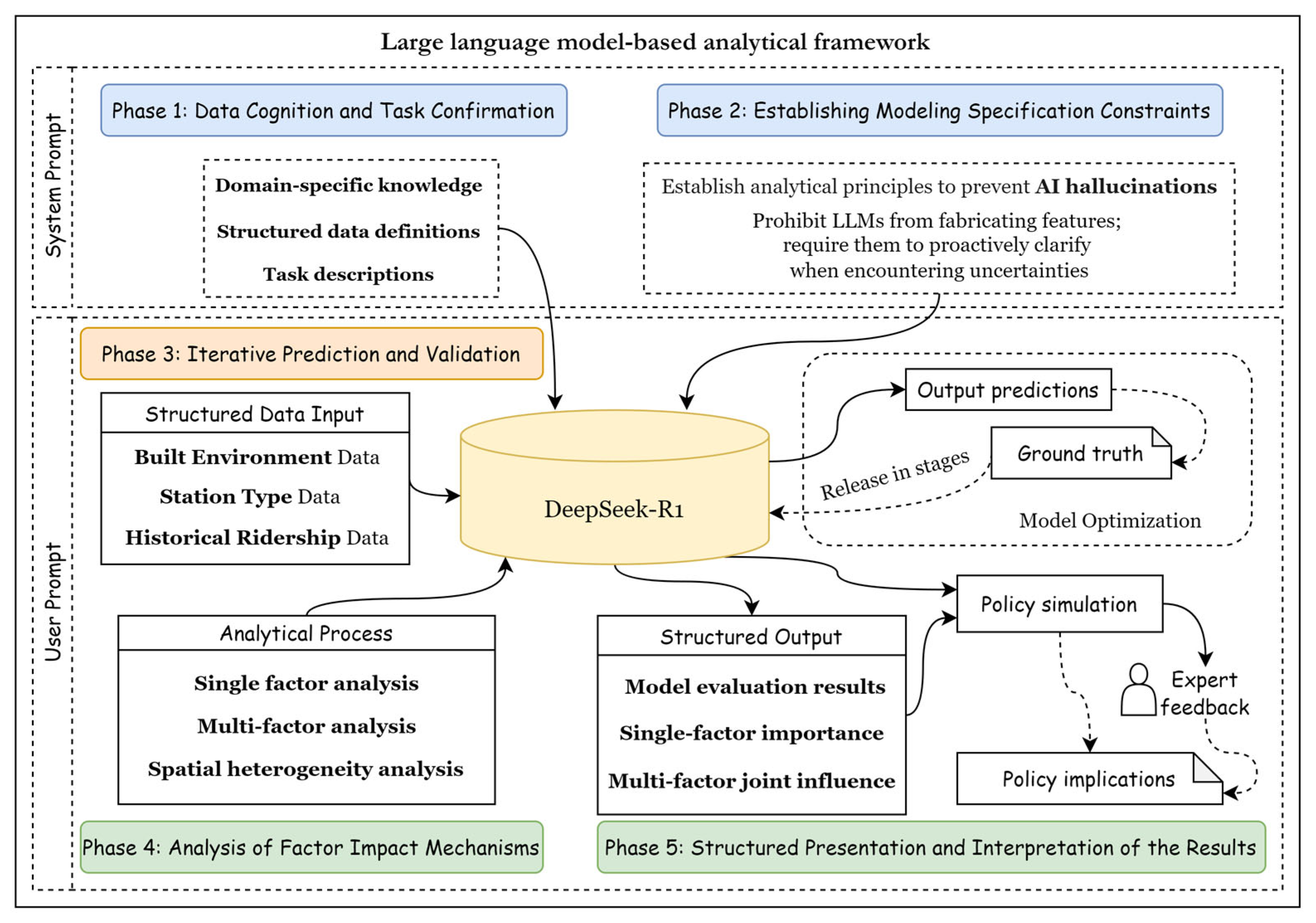27]. Additionally, to address potential AI hallucinations and ensure reliability and interpretability in LLM modeling, this study designs a five-stage analytical framework using a chain-of-thought prompting strategy. Each stage is executed and validated independently before proceeding to the next, ensuring reliability through multiple interactions. The specific framework structure is shown in Figure 3. The following sections describe the specific content of each of the five stages.

4.2. Prompt Construction

Data Cognition and Task Confirmation (Phase 1): The first stage encompassed domain-specific knowledge, structured data definitions, and clear task descriptions. Domain-specific knowledge includes the definition of the model’s role (e.g., “You are a professional transit ridership prediction model that can forecast future ridership based on the built environment characteristics around metro stations”), as well as definitions of transit ridership, peak hours, and Pedestrian Catchment Areas (PCAs). Structured data definitions include descriptions of the physical meanings and abbreviations for the built environment and station type factors, as well as historical ridership data, along with their respective input formats. Finally, specific tasks were clearly defined, including utilizing the aforementioned structured data to predict the peak ridership for workdays in the upcoming week and analyzing the influence and interaction mechanisms of the built environment factors and station type factors for weekday peak ridership further.

Establishing Modeling Specification Constraints (Phase 2): After ensuring that DeepSeek had accurately understood the data structure, domain knowledge, and task requirements, we established a set of constraint specifications for the LLM to guide the entire interpretation process to minimize AI hallucinations. The specifications included four components: First, its reasoning had to be based on the structured data provided, and fabricated features that could influence the results were prohibited. Second, regarding the numerical predictions, the LLM was directed to decompose the task into two steps: initial temporal pattern recognition, which considered the day-of-week patterns and the week-over-week patterns in historical data, followed by an analysis of how the station-specific built environment features and station type factors influenced ridership. Third, guidance was provided on conducting an analysis of influencing factors, encompassing both single-factor impact analysis and multi-factor interaction analysis. The detailed analytical methods will be introduced in Phase 4. Finally, the LLM was required to actively seek clarification when encountering uncertain information throughout the analysis process. By establishing these specification constraints, the LLM was guided to conduct an accurate analysis while minimizing fabricated results. Phase 1 and Phase 2 jointly form the system prompts, with Figure 4 comprehensively depicting the detailed composition of these prompts.

Iterative Prediction and Validation (Phase 3): This stage involved inputting historical ridership data, built environment data, and station type data into the LLM according to the format described in Phase 1. The LLM was required to output prediction results in a specified format. After the LLM outputs the results (predicting the five working days of the upcoming week), the ground truth for the first three days is provided to the LLM, allowing it to validate the existing model and make improvements before regenerating the results for the remaining two days, thus implementing a dynamic optimization mechanism.

Analysis of Factor Impact Mechanisms (Phase 4): After completing the prediction and model optimization, we further guided the LLM to conduct a factor analysis to explain the mechanisms of the influence of various variables on transit ridership. We designed an analytical process for the LLM that included three aspects: First, a single-factor analysis, which quantified the relative importance of the different factors. Specifically, for each variable, counterfactual scenarios were generated (with all of the other variables held constant), and the LLM was used to predict the resulting change in ridership. The magnitude of this change was then used to compute the relative importance of the variable. Second, a multi-factor interaction analysis (including synergistic or antagonistic effects) was conducted by generating counterfactual scenarios with different combinations of selected variables. Changes in predicted ridership under these scenarios were then used to assess the joint impact of the selected variables. It is important to note that in the presence of multicollinearity among variables, feature disentanglement is required, achieved through dynamic allocation of the attention weights. In such cases, the LLM selects dominant variables based on the specific context. For example, if “stores” and “land use mix” are highly correlated, the LLM may place greater emphasis on “stores” in CBD areas, while focusing more on “land use mix” in suburban areas. Third, a further analysis of spatial heterogeneity was made (for example, comparing the similarities and differences in the single-factor and multi-factor interactions between CBD stations and non-CBD stations). This process encompasses both macro-level (network/system level) and micro-level (station level) perspectives to comprehensively analyze the influence mechanisms of the built environment and station type factors on transit ridership.

Structured Presentation and Interpretation of the Results (Phase 5): After completing the analysis process of the previous four stages, we required the LLM to manage the results into a structured output format, facilitating more intuitive continued interpretation and summarization of the LLM’s findings and their implications. This section primarily consists of three aspects. The first part involves outputting performance metrics (including the MAPE, R², and A20 index) for the model evaluation according to four types of peak ridership. The second part is factor impact evaluation and key interaction identification, which includes the relative importance (0–9) of the different factors for various peak ridership types, as well as the interactions between multiple factors, outputting the results in tabular form. The third part involves policy simulation and policy recommendations based on the results of the previous analysis, where the LLM provides policy-oriented suggestions.

4.3. Evaluation Metrics

To validate the reliability of the DeepSeek-based predictions and analyses, we evaluated the model performance using three key metrics: the mean absolute percentage error (MAPE), the coefficient of determination (R²), and the A20 index (formulas are provided below).

The MAPE measures the average percentage error between the predicted and actual values, providing an intuitive interpretation of the prediction accuracy. A lower MAPE value indicates a better performance of the model.

$$\mathrm{MAPE}={\displaystyle \frac{1}{n}}\sum _{i=1}^n\left|{\displaystyle \frac{y_i-{\widehat{y}}_i}{y_i}}\right|\times 100$$

(2)

R² quantifies the proportion of the variance in the dependent variable that is explained by the independent variables. It ranges from 0 to 1, where a higher value indicates a better model fit.

$${\mathrm{R}}^2=1-{\displaystyle \frac{\sum {({\widehat{y}}_i-y_i)}^2}{\sum {(y_i-\overline{y})}^2}}$$

(3)

The A20 index measures the proportion of the predictions that fall within ±20% of the actual values. A higher A20 value indicates a better predictive accuracy.

$$\mathrm{A}20 \mathrm{index}={\displaystyle \frac{{\displaystyle \sum _{i=1}^n}I\left(\left|\frac{y_i-\widehat{y_i}}{y_i}\right|\le 0.2\right)}{n}}\times 100\%$$

(4)

where ${\widehat{y}}_i$ represents the predicted value of the model, $y_i$ represents the actual value, n represents the number of samples, $\overline{y}$ is the mean of the actual values, and I(·) is an indicator function that equals 1 if the condition is met and 0 otherwise.

To assess whether built environment (BE) factors contributed to improving the prediction accuracy, we compared the results of the LLM with BE factors and those of the LLM without BE factors. Furthermore, to verify the effectiveness of the LLM-based predictions, we conducted a comparative analysis against the ARIMA model and the widely adopted machine learning model XGBoost. The detailed validation results are discussed in Section 5.3.

5. Results and Discussions

Through the LLM-based analytical framework described in Section 4, we conducted multiple rounds of interactions with DeepSeek-R1 to obtain comprehensive results on the impact of built environment factors and station type characteristics on the weekday peak-hour transit ridership. We have organized the discussion of the model’s analytical outputs into two subsections: the relative importance analysis of the variables and the multi-variable interaction analysis.

5.1. The Relative Importance of the Variables

The analysis of the relative importance of the variables includes both macro-level and meso-level perspectives. At the macro level (at the network level/across all stations), it examines the relative importance of built environment and station type factors. The results are first presented for overall peak-hour ridership in Figure 5, followed by different peak-hour ridership types (MB/MA/EB/EA) in Figure 6, Figure 7, Figure 8 and Figure 9. At the meso level, different types of stations, including terminal and transfer stations (defined by the transit network operational data), CBD stations (determined by whether a station is located in the CBD), and suburban and recreational stations (inferred by the LLM from multidimensional built environment features such as the POI density and demographic metrics), are examined, with the top five ranking of the factor importance for each station type detailed in

Table 3. Top five important variables for different types of stations with relative importance.

Relative Importance Ranking	Terminal Stations	Transfer Stations	CBD Stations	Suburban Stations	Recreational Stations
1	Population density (9.0)	Transfer dummy (9.2)	Stores (9.1)	Distance to city center (9.1)	Recreation (9.2)
2	Residences (8.2)	Bus lines (8.5)	Office towers (8.8)	Population density (8.4)	Land use mix (8.4)
3	Bus lines (7.5)	Stores (8.1)	CBD dummy (8.3)	Residences (8.1)	Intersections (8.2)
4	Land use mix (7.1)	Office towers (7.8)	Housing price (7.2)	Recreation (7.4)	Stores (7.9)
5	Stores (6.8)	Road density (7.3)	Intersections (6.9)	Land use mix (6.5)	Road density (7.5)

.

In the radar charts of the overall and MB/MA/EB/EA ridership, distinct patterns of factor importance were observed. The MA radar chart displayed the most pronounced peak, representing the CBD dummy variable. The EB radar chart exhibited three distinct peaks, corresponding to the CBD dummy variable, land use mix, and bus lines. In contrast, the EA flow radar chart showed no prominent peaks, indicating a more balanced influence across various factors. Both the overall and MB radar charts highlighted population density and residence as important factors, while station-specific factors such as the CBD dummy variable (in the overall radar chart) and the terminal dummy variable (in the MB radar chart) also demonstrated high importance. The following paragraphs discuss the relative importance of these different variables in detail.

The two most important factors overall were the CBD dummy variable and population density. The CBD dummy variable exhibited the highest importance among the overall, MA, and EB ridership, while population density showed the maximum importance to MB ridership. This suggests that commuting trips related to employment in the CBD area were predominant, which is consistent with the findings of many studies [10,49]. However, some research indicates that proximity to the CBD is not always a significant factor [16,44]. Furthermore, beyond the commuting population, Zhang et al. [50] also found that distance to the CBD has a significant impact on disadvantaged groups. Distance to the city center moderately influenced both MB and EA ridership, with a slightly higher impact on EA. Bus lines demonstrated more significant effects on morning peak ridership. Residences showed high importance to the MB and EA ridership, while companies and office towers had stronger influences on the EB and MA ridership. These patterns confirm that the peak-hour ridership was primarily driven by commuting behavior, with the MB/EA ridership reflecting morning departures from homes to workplaces and evening returns, while the MA/EB ridership represented arrivals at workplaces and evening departures.

The land use mix and bus stops showed a higher importance to EB ridership but had relatively limited effects on the other types of ridership. The transfer dummy variable had a considerable influence on MA ridership but showed a limited impact on the other types of ridership. Although the terminal dummy variable showed relatively low importance at the overall level, it had a considerable impact on MB ridership.

In EA ridership, beyond residences, commercial variables such as stores, recreation facilities, restaurants, and living services also demonstrated relatively high importance. In addition, factors reflecting walkability, such as intersections and road density, showed similar levels of importance. This suggests that EA ridership was not solely commuting-driven but also partially leisure-driven.

Regarding the relative importance of different types of stations, first, the two most important factors in terminal stations and suburban stations were population density and residences, indicating that suburban areas are still primarily residential. Second, the land use mix also showed high importance across most station types (with a relative importance from 6.5 to 8.4). Third, bus lines had a significant influence on terminal stations and transfer stations (the relative importance was 7.5 and 8.5, respectively). Fourth, for the recreational stations, intersections and road density demonstrated relatively high importance, suggesting that enhancing the walkability around these stations could promote walking, cycling, and metro travel while reducing the dependence on private vehicles. Additionally, in the CBD stations, stores exhibited a similarly high importance to that of office towers, indicating that the land development in CBD areas is more balanced, with a higher degree of mixed use.

5.2. The Multivariate Interaction Analysis

The multi-variable interaction analysis encompasses both key factor combinations and latent factor combinations. Key factor combinations refer to variables that demonstrate a high relative importance in a single-factor analysis and exhibit either synergistic or antagonistic effects on peak-hour transit ridership. Latent factor combinations, conversely, consist of factors that appear insignificant in isolation (with low single-factor importance) but drive substantial ridership changes when interacting with others. Figure 10 visually depicts the key and latent factor combinations discovered by DeepSeek. The color intensity and arc length of each factor represent their respective importance, arranged in descending order of importance in a counterclockwise direction. The CBD dummy variable has the highest importance, while companies, road density, and living services are the factors with the lowest importance.

Table 4. Key factor combinations and expected impacts.

Key Factor Combinations		Impact Quantification	Synergistic (S)/Antagonist (A)
CBD dummy	Stores↑	C3 > 75, MA increases up to 18%	S
	Office towers↑	Office towers > 9, EA increases up to 12%	S
Distance to city center↑	Land use mix↓	Distance to city center > 11, land use mix < 0.55, MA decreases up to 15%	A
Distance to city center↓	Land use mix↑	Distance to city center < 2, land use mix > 0.6, EA increases up to 16%	S
Transfer dummy	Bus lines↑	Bus lines > 20, EB increases up to 22%	S
Intersections↑	Stores↑	Intersections > 25, stores > 50, EB increases up to 9%	S
	Recreation↑	Intersections > 25, recreation > 70, EB increases up to 21%	S

presents the key factor combinations and provides a quantitative assessment of their impacts on peaktransit ridership. Although the quantification of the interaction impacts only reports the magnitude of the change in ridership without specifying individual stations, the intermediate outputs of the LLM include station-level information. For example, in Table 4, the synergistic effect between the “transfer dummy” variable and “bus lines” shows that when the number of bus lines exceeds 20, the EB ridership at Station 17, which is a transfer station, increases most significantly, by up to 22%. In contrast, at Station 4, which is not a transfer station, the increase is only 3%. Therefore, the final reported conclusion is based on the maximum observed increase, that is, an increase of up to 22%. The CBD dummy variable, which ranks highest in relative importance, shows its two most significant synergistic interactions with stores and office towers. The positive influence of increased stores on MA ridership may be attributed to two primary drivers: First, a higher commercial density creates additional employment opportunities, and second, CBD-area stores provide breakfast, coffee, and other services that attract commuters to exit stations. The enhancement of EA ridership by office towers can be readily explained by their multifunctional nature, which frequently incorporate supplementary commercial facilities such as shopping malls and restaurants rather than these serving exclusively as corporate offices. The combination of the distance to the city center and land use mix demonstrates both synergistic and antagonistic effects. In suburban stations, the low land use mix further reduces MA ridership, whereas central stations with high mixed-use development attract greater EA ridership. Although some empirical studies have found the effect of the distance to the city center on transit ridership to be insignificant, the majority of the research suggests its significant impact, though the threshold varies across regions. For example, in the Washington metropolitan area, the effect of the distance to the city center on ridership becomes negligible when it exceeds 5 km [23]. A case study by Liu et al. of Jinan, China, found that when the distance exceeds 12 km, car dependence increases significantly, while public transit usage declines [51]. Both Jinan and Qingdao are located in Shandong province, China, with Jinan serving as the provincial capital and Qingdao as the most economically developed coastal city in this region. The two cities share similar urban scales. Notably, DeepSeek identified a threshold of 11 km, which closely aligns with the findings for Jinan. This consistency further supports the validity of LLM-based analyses. Another dummy variable, for transfer stations, works synergistically with bus lines to increase EB ridership. Lastly, high intersections show significant positive interactions with both stores and recreational facilities in influencing EB ridership, suggesting that dense street networks shorten walking distances and attract non-commuting passengers to choose metro transportation.

The latent factor combinations and their estimated impacts are presented in

Table 5. Latent factor combinations and expected impacts.

Latent Factor Combinations (* Represents a Low-Importance Factor)		Impact Quantification	Synergistic (S)/Antagonist (A)
Distance to city center↑	Living services↑ (*)	Distance to city center > 9, living services > 65, EA increases up to 7%	S
Road density↑ (*)	Living services↑ (*)	Living services > 45, road density > 7, EA increases up to 11%	S
Road density↓ (*)	Recreation↑	Recreation > 120, road density < 6, EB decreases up to 12%	A
Road density↑ (*)	Companies↑ (*)	Companies > 70, road density > 8, EB increases up to 19%	S
Land use mix↓	Companies↑ (*)	Companies > 150, land use mix < 0.5, MA decreases up to 8%	A

. First, road density exhibits a relatively low importance, showing slight significance only for recreational stations. However, when interacting with other factors such as living services and companies, it significantly influences ridership patterns. In areas with a high density of recreation facilities but a low road density, the EB ridership still decreases. Conversely, a high road density synergistically enhances EA ridership when combined with living services and similarly promotes EB ridership when interacting with companies. These findings suggest that a high road density improves pedestrian accessibility, potentially constrains the efficiency of vehicular traffic, and increases the popularity of the metro. Furthermore, evening work shifts or after-work activities become more accessible with good road connectivity. Second, living services also demonstrate relatively low importance individually. However, in suburban stations, a greater concentration of living services can boost EA ridership. Finally, even with a higher number of companies, MA ridership remains negatively affected when the land use mix around stations is low. This observation further emphasizes the significance of mixed-use development in enhancing metro ridership.

Therefore, when considering the policy implications, we should leverage synergistic effects while mitigating antagonistic interactions. For instance, appropriately increasing the commercial facilities within the PCAs of CBD stations would be beneficial. Similarly, optimizing the number of bus lines within the PCAs of transfer stations and enhancing the integration between bus and metro services could improve ridership. Moderately increasing the road density and intersections would promote pedestrian-friendly environments, thereby enhancing the attractiveness of metro transportation. Additionally, it is advisable to avoid single-use land development patterns near suburban stations, such as an excessive concentration of residences or industrial agglomeration. Regarding the latent factor combinations, we can formulate several policy measures. For instance, implementing a flexitime policy in conjunction with well-connected road networks and pedestrian-oriented infrastructure designed for accessibility, including wide sidewalks, continuous obstruction-free pedestrian pathways, intuitive crosswalks with adequate timing of signals, and seamless connections to metro stations, could encourage greater use of public transit. Moreover, the availability of living services around metro stations also relies on improved street connectivity to further incentivize more people to adopt public transportation modes.

5.3. Validation

To validate the effectiveness of the DeepSeek-based model in understanding the built environment and predicting transit ridership, we conducted comparative experiments between the LLM predictions and classical models. Four modeling approaches were evaluated according to their transit ridership predictions: the proposed LLM-based model, an ablated version of the LLM without the built environment (BE) factors, the XGBoost model, and the ARIMA model. The performance was assessed using the MAPE, R², and A20 index.

The proposed LLM model with BE factors demonstrated a more robust performance across all evaluation metrics (

Table 6. Model performance in comparative experiments.

Model	Metric	Morning Boarding	Morning Alighting	Evening Boarding	Evening Alighting	Overall
LLM with BE factors	MAPE (%)	11.2	13.4	14.1	12.5	12.8
	R2	0.91	0.88	0.87	0.90	0.89
	A20 index (%)	89.2	86.8	85.9	88.1	87.5
LLM without BE factors	MAPE (%)	14.8	16.2	16.9	14.5	15.6
	R2	0.85	0.83	0.82	0.86	0.84
	A20 index (%)	83.5	81.4	80.8	83.5	82.3
XGBoost	MAPE (%)	14.8	16.2	17.5	15.6	16.0
	R2	0.87	0.85	0.84	0.86	0.86
	A20 index (%)	84.6	83.2	82.5	83.8	83.5
ARIMA	MAPE (%)	18.7	20.3	21.5	19.8	20.1
	R2	0.83	0.81	0.80	0.82	0.82
	A20 index (%)	79.5	77.2	76.8	78.4	78.0

). With an overall MAPE of 12.8%, R² of 0.89, and A20 index of 87.5%, it showed enhanced accuracy and stability compared to XGBoost (MAPE: 16.0%, R²: 0.86) and ARIMA (MAPE: 20.1%, R²: 0.82). The ablated LLM model without the BE factors exhibited a reduced performance (MAPE: 15.6%, R²: 0.84), emphasizing the crucial role of environmental features such as land use and external connectivity. While the XGBoost model ranked second with moderate accuracy, the ARIMA model consistently showed the lowest performance due to its limitations in incorporating non-temporal factors.

Regarding the boarding patterns, morning boarding showed the highest predictability across all models, with the LLM achieving an MAPE of 11.2% and R² of 0.91, performing notably better than XGBoost (14.8%, 0.87) and ARIMA (18.7%, 0.83). This observation aligns with the regularity of morning commuter schedules. Conversely, evening boarding ridership presented the greatest challenge, with even the LLM showing an MAPE of 14.1%, possibly due to the diverse purposes of trips during evening peaks. Interestingly, the LLM without the BE factors performed slightly worse than XGBoost in its EB predictions (MAPE: 16.9% vs. 17.5%), suggesting that tree-based models may handle temporal patterns more effectively when environmental data are unavailable.

For the alighting patterns, evening alighting ridership showed better predictability than that of evening boarding (LLM MAPE: 12.5% vs. 14.1%), likely reflecting more consistent return-home behaviors. Morning alighting ridership displayed intermediate variability (LLM MAPE: 13.4%), potentially influenced by flexible work schedules.

The LLM’s advantage lies in its capability to integrate environmental factors with temporal dynamics, achieving 21.9% and 25% reductions in the MAPE compared to that of the LLM without the BE factors (from 15.6% to 12.8%) and XGBoost (from 16% to 12.8%), respectively.

6. Conclusions

This paper introduces a DeepSeek-powered LLM-based analytical framework to interpret the impact of built environment factors and station characteristics on peak-hour metro ridership. The methodology employs a chain-of-thought prompting strategy, where each stage is independently executed and validated before progression, ensuring reliability through multiple interactions. Modeling specifications and constraints were established for the LLM to minimize AI hallucinations. To validate both the effectiveness of the built environment factors and the reliability of the LLM-based model, comparative experiments were conducted among four models: the LLM with BE factors (our model), the LLM without BE factors, XGBoost, and ARIMA. The results demonstrate that our model achieves the optimal performance, while the LLM without the BE factors performs slightly worse than XGBoost, indicating that the LLM correctly understands and models built environment factors, while confirming the reliability of the LLM’s prediction results.

Our study provided the following key merits and implications. First, unlike the conventional machine learning models and linear regression models, the LLM can understand the physical significance of the built environment and station type factors, avoiding the modeling difficulties that arise when the classical models consider too many overlapping indicators. Second, we proposed an LLM-based analytical framework that progressed in stages and ensured analytical reliability through multiple rounds of interaction. Furthermore, the fully open-source nature of DeepSeek-R1, along with its ability to display the complete process of reasoning, ensures the interpretability and transparency of the entire prediction and analysis workflow. Third, this paper considers not only the influence of single factors on peak ridership but also examines their joint influence, identifying several key factor combinations. Fourth, we also consider hidden drivers—factors that appear insignificant in isolation (with low single-factor importance) but drive substantial changes in ridership when interacting with others. For example, road density shows low relative importance individually but can produce both synergistic and antagonistic effects on ridership when combined with other factors. Lastly, the proposed DeepSeek-based analytical framework is highly adaptable and could be applied to other regions, as well as to different transportation modes, such as bike-sharing systems and bus transit, or even forecasting and analysis of the multimodal transportation demand.

Our model has several limitations that highlight important directions for future research. First, the delineation of the PCAs in our study was based on the Euclidean distance. Although this is the most commonly used method in the literature, some scholars argue that the Euclidean distance is relatively simplistic and may not accurately reflect real-world conditions [6]. Alternative measures, such as the road network distance, which represent actual walking paths better, may yield different conclusions. Second, the POI data input into DeepSeek were preprocessed and aggregated, containing only numerical counts without specific names, which may have led to the loss of valuable information. For example, the impact of parking in our model was negligible, potentially due to the limitation of the POI counts in accurately representing the actual number of parking spaces. Therefore, future studies could explore the design of supervised fine-tuning tasks that enable LLMs to learn how to extract key built environment features from unstructured text. This approach could help preserve more useful information within the data, potentially improve the computational efficiency, and reduce the resource consumption. Third, we lacked certain critical data, such as employment density data, which could, jointly with population density, positively influence transit ridership [52]. By integrating additional data sources, such as location-based service (LBS) data and floor area ratio (FAR) data, researchers may uncover more insightful and meaningful findings. Lastly, the metro ridership data used in our study were relatively outdated and limited in their station coverage, which may have impacted the robustness of the results of our analysis.

Future research could expand the existing framework by first incorporating comparative studies that examine intra-city regional disparities, alongside cross-city analyses of diverse urban contexts such as megacities like Shanghai and mid-sized cities like Qingdao, to determine whether the factors identified and their relationships with transit ridership are universal or context-dependent. Given the long-term impacts of the built environment on ridership, the framework could also be extended through a longitudinal trend analysis to exploring the historical dynamics between the built environment metrics and ridership patterns, as well as the effects of urban policies and planning interventions. This approach will require data spanning extended periods, but it could help uncover the co-evolutionary patterns between the built environment and transit ridership. Additionally, the micro-level analysis could be deepened through station-specific studies and pedestrian-level assessments of how physical environments influence walking to/from metro stations. Furthermore, integrating qualitative data would enrich the framework by capturing users’ subjective experiences of the built environment, including their perceptions of time costs such as perceived walking time to stations or the reliability of waiting times, thereby revealing psychological and social factors beyond quantitative metrics to holistically understand the interactions between urban form and metro use. Finally, to extend the proposed framework to scenarios with limited open-source data (small cities, suburban areas) and other transportation modes with unstructured domain knowledge (e.g., shared bikes, customized buses), it is necessary to enhance the LLM’s unstructured data extraction capabilities further. This could be achieved by pre-training the LLM on general domain knowledge and applying few-shot fine-tuning to reduce its dependence on large-scale data. For example, when analyzing suburban bus stops, transfer learning can reuse the experience from models trained on urban central areas, combined with local parameter adjustments based on unique suburban characteristics (e.g., a lower population density, longer commute distances), to improve the LLM’s robustness in data-sparse or complex scenarios.

In conclusion, the mechanisms through which the built environment influences various transportation modes remain a crucial topic for further research. With the continuous advancement of LLMs’ reasoning capabilities, LLMs can be leveraged to consider a broader range of influencing factors and explore their joint influence. These findings provide valuable insights for transportation planners and policymakers, offering guidance on policy implications. Furthermore, they can contribute to promoting land use intensification, increasing the modal share of public transport, reducing transportation-related carbon emissions, and ultimately enhancing the overall sustainability of the transportation system.