Abstract
This study investigates the reliability of tall buildings subjected to dynamic across-wind loading, focusing on the Tuned Mass Damper Fluid Inerter (TMDFI). While existing literature emphasises the effectiveness of TMDFI in mitigating seismic hazards, research on its reliability regarding wind hazards remains limited. A wind-sensitive benchmark 76-storey building is modeled to compare the performance of the TMDFI against a traditional tuned mass damper (TMD) and an uncontrolled structure. A Monte Carlo Simulation (MCS) approach comprising 31,500 simulations is employed to assess reliability under uncertain damping ratios and varying turbulence intensities at reference wind speeds of 20 to 40 m/s. Key performance metrics, including peak acceleration and root mean squared (RMS) displacement responses, are derived through spectral analysis in the frequency domain. Results indicate that the TMDFI offers superior reliability, allowing an additional 6–7 m/s in reference velocity before reaching significant failure at the ISO limit state. Peak acceleration and RMS displacement are reduced by up to 64% to the uncontrolled structure. The TMDFI consistently outperforms both the TMD and uncontrolled configurations across all turbulent cases and wind velocities examined.
1. Introduction
Tall buildings face unique design challenges due to their increased sensitivity to dynamic wind loading. As building height increases, structural stiffness typically decreases, resulting in lower natural frequencies that can align with the energy-rich, low-frequency components of turbulent wind spectra [1]. Simultaneously, the wind speed, and hence aerodynamic load, increases with height due to the wind shear effect, amplifying the dynamic excitation of upper floors. This combination can lead to significant across-wind responses, vortex shedding, and resonance phenomena, particularly in flexible, slender structures commonly found in modern cities.
Wind-induced vibrations in tall buildings can affect structural performance, compromise occupant comfort, and disrupt the operation of sensitive equipment on upper floors. As architectural and urban trends continue to favor taller, more flexible structures, these challenges become more pronounced. In such systems, damping plays a critical role in controlling dynamic response, often serving as the primary mechanism for mitigating wind-induced motion. Accurate estimation and effective utilization of damping are therefore essential to ensure safety, serviceability, and occupant well-being under wind loading. However, despite decades of advancement in structural dynamics, the accurate estimation of damping in tall buildings remains an unresolved challenge. As noted by Kareem and Gurley [2] in the classical text on the subject, reliable damping values are often only obtainable post construction, and this uncertainty continues to necessitate probabilistic approaches in response prediction and vibration control design. Determining the precise level of structural damping in a structure is challenging, often involving the installation and design of complex monitoring systems and algorithms [3,4,5]. In many tall, flexible buildings, the inherent structural damping is often insufficient to effectively mitigate structural vibrations [6]. If inherent structural damping is insufficient to control wind-induced vibrations, engineers must design and implement auxiliary damping devices, such as tuned mass dampers or fluid viscous dampers, to supplement energy dissipation and achieve acceptable performance levels [7]. Experimental studies conducted in the past few years have shown that installing dampers can increase the first-mode damping ratio by more than 500% [8]. This substantial enhancement in damping underscores the critical role of dampers in improving the dynamic performance of tall buildings.
Damping devices used for vibration control in tall buildings are typically classified as passive, semi-active, active, or hybrid systems. Passive dampers, such as tuned mass dampers (TMDs), operate without external power and rely on mechanical properties to dissipate energy. The passive TMD is the most commonly used auxiliary damper and is installed in many of the world’s tallest buildings [9,10], including in super-tall buildings [11] and in tall modular structures [12]. Passive dampers are simple, reliable, and low-cost. They are activated by the motion of the structure and require no power source to operate. In recent studies, passive TMDs have been shown to perform well in tall buildings under wind loads [13,14]. Other passive dampers such as tuned liquid dampers (TLDs) [15,16] and tuned liquid column dampers (TLCDs) [17] have also been proposed in recent years. Semi-active systems adjust their properties in real time based on structural response but do not add energy to the system [9]. Semi-active TMDs have been used for wind-induced vibration control of tall buildings [18], and magnetorheological (MR) [19,20] dampers have been utilized for this purpose, too. Active control systems, such as active mass dampers (AMDs), apply external energy through actuators to counteract structural motion, enabling precise control but requiring continuous power and complex control algorithms [21]. Active tuned mass dampers (ATMDs) have been used to mitigate wind induced vibrations in multistorey buildings [22]. Recently, an ATMD system was proposed and installed in a 600 m tall skyscraper to suppress wind-induced building vibrations [23]. AMDs have also been used for vibration control of tall flexible structures subjected to wind loads [24]. Hybrid systems combine elements of active and passive control, offering a balance between energy efficiency and adaptability; for example, a hybrid mass damper may use a passive TMD supported by active feedback control to enhance performance across a wider range of excitation conditions [25]. These types of damping systems have been used in recent studies to suppress wind-induced vibration of tall buildings such as hybrid TLCDs [26] and hybrid TMDs [27].
The performance of damping systems in tall buildings depends on their type, mass, and stroke length. Passive dampers are simple and reliable but require large mass and stroke, offering modest vibration suppression. Semi-active and active systems provide better control and adaptability, with increased stroke lengths for enhanced performance, but they introduce complexity, power reliance, and higher costs. Hybrid systems balance these traits, though they still require some external input and tend to be complex to design and maintain [25].
Recently, inerter-based systems have been widely investigated and implemented to mitigate wind-induced motions in tall buildings [28]. Inerter-based dampers amplify inertial effects without added damper mass, achieving superior vibration suppression compared to traditional dampers across a wide frequency range. With less mass required and reduced stroke lengths, they offer efficient, effective vibration control, making them a practical evolution in structural control for tall buildings. Initially proposed by Smith [29], the ideal inerter is a linear mass-less two-terminal mechanical element resisting the relative acceleration at its terminals through an inertance coefficient, b, measured in units of mass.
The inerter behaves as an inertial weightless element whose gain depends on the relative acceleration observed by its terminals and its inertance. A TMD coupled with an inerter has been used in several studies for vibration control of tall flexible structures such as buildings, wind turbine blades, and towers [30,31,32,33]. Recently, the Tuned Mass Damper Fluid Inerter (TMDFI) has seen interest in the literature for both the seismic control of structures [34] and for the attenuation of wind-induced vibrations [35,36] in tall flexible structures. The fluid inerter device consists of a piston, encased in a cylinder containing fluid. When the piston moves through the cylinder, it forces fluid through a helical coil channel which generates a resistive force due to the inertia of the moving fluid. Due to the presence of the helical channel, a portion of this resistive force is proportional to the acceleration of the piston and therefore the relative acceleration of the chosen inerter terminals [37]. A diagram of the idealised fluid inerter device is shown in Figure 1, with the key fluid inerter design parameters given in Table 1.
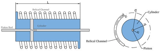
Figure 1.
Ideal fluid inerter, adapted from [34].

Table 1.
Physical Properties of the Helical Fluid Inerter.
Considering the geometric properties of the fluid inerter, the inertance b required to determine the inertance force may be approximated as
Recently, notable applications of reliability theory in inerter-based dampers have been proposed. Much of the literature has investigated the reliability of these devices under seismic actions. Giaralis and Taflanidis [38] and Ruiz et al. [39] both employed Monte Carlo Simulations, finding that TMDIs offer enhanced structural control and outperform TMDs in reducing damage. Petrini et al. [40] and Zhou et al. [41] used Uncertain Parameter Variation methods, showing that TMDIs can maintain or improve occupant comfort and structural reliability even under uncertain parameters, particularly when the inertance is sufficiently large. Most recently, Peng and Sun [42] used the probability density evolution method, confirming that optimally designed TMDIs provide superior control to TMDs at the same mass ratio, especially under stochastic excitation conditions.
Aims of This Study
Having presented the literature on the dynamics of tall buildings, the use of damping devices, and their reliability under various loading conditions, we now aim to investigate the effectiveness of the Tuned Mass Damper Fluid Inerter (TMDFI) in improving structural reliability under dynamic across-wind loading. While much of the existing research has focused on its application for mitigating seismic hazards, this study seeks to fill the gap in understanding its performance in wind-sensitive environments. By comparing the TMDFI to both a traditional tuned mass damper (TMD) and an uncontrolled structure, we aim to assess its potential to enhance structural performance and reliability under uncertain damping properties and varying wind conditions.
2. Methodology
This paper uses the 76-storey building proposed in [43] as a benchmark model. The structure has a height of 306.1 m and a total mass of 153,000 metric tons. The building has a square plan area with a depth (D) and breath (B) of 42 m. The structure is slender with an aspect ratio of , rendering it particularly susceptible to wind effects. Both the plan and elevation of this benchmark structure are shown in Figure 2.

Figure 2.
Elevation and plan view of the benchmark structure, adapted from [43].
The 76-storey building is modeled as a vertical cantilever using Bernoulli–Euler beam theory. A finite element model of the structure is constructed by considering the portion of the building between two adjacent floors as a classical beam element of uniform thickness. This results in a model with 76 degrees of freedom (DOF) (translational). The first three calculated natural frequencies of the 76-DOF model are and Hz.
The input across-wind action to the 76-DOF model is computed using the across-wind model developed in [44]. This model captures the vortex shedding frequency within the overall across-wind model. For structures square in plan such as this, the vortex shedding frequency emerges as an obvious peak on the across-wind power spectrum, with the overall spectrum dominated by this effect, therefore having the appearance of a single peak. The model proposes that the diagonal terms of the across-wind power spectrum matrix are given as
which specifies the power spectral density (PSD) of the floor. The parameters involved in Equation (2), as outlined in [44], are
where is the mean of the RMS lift coefficient of the rectangular building, and are experimentally determined parameters corresponding to the spectrum bandwidth, is the root mean square (RMS) of the across-wind force, z is the height of the floor from ground level, is the vortex shedding frequency in rad/s, is the Strouhal number, S is the cross-sectional area of the building, is the air density taken as 1.225 kg/m3, and is the tributary height of the floor. is the mean wind speed at height z above the ground level given as
where represents the reference velocity (commonly referred to as the design wind speed), is the reference height at which this reference speed is taken. For this study, is assumed to be 810 m, representing the characteristic height of the atmospheric boundary layer [40]. represents the dimensionless shear exponent that depends on the terrain’s surface roughness and is assumed to be , corresponding to a congested urban area [45]. To effectively model the off-diagonal terms of the across-wind power spectra, Ref. [44] proposes a vertical coherence function . This function is obtained from wind tunnel testing and appears in the model to correct for the vertical decay in the co-spectra of across-wind forces between two floors as the distance between the floors increases. The coherence function used is given as
where and are the heights of the floors considered and is the experimentally determined coefficient determining the rate of decay, taken as . This yields an overall across-wind force power spectral density function of
Although the model above is deterministic in nature and is rooted in empirical data, for the purpose of a reliability assessment, both the reference velocity and the turbulence intensity are varied. The reference velocity is varied from 20 m/s to 40 m/s at a constant 1 m/s interval. The range of wind velocities considered is selected with aims of encapsulating extreme wind loading conditions across differing regions with varying levels of wind exposure. The turbulence intensity is varied by considering three cases: a low-turbulence case, a medium-turbulence case, and a high-turbulence case. This discretization of turbulence intensity is taken to maintain the computational tractability of the model. The turbulence intensity values selected for this study are presented Table 2.
Table 2.
Chosen Turbulence Intensity Values.
The turbulence intensity approach utilized in this study represents a simplification of the complex process below the atmospheric boundary. The three selected turbulence intensity values are taken as constant along the height of the buildings. The turbulence intensity plays a key role in shaping the power spectral density (PSD) of wind loads, particularly in across-wind direction. In the current study, turbulence intensity influences the variance of fluctuating wind speeds at each height and therefore directly affects the magnitude of the aerodynamic force spectra.
Specifically, the PSD of wind-induced lift forces is proportional to the square of the local turbulence intensity, as seen in the formulation adapted from Gu and Quan [46], where the spectral density at each height is computed as
This relationship implies that higher turbulence intensity leads to larger fluctuating force components and thus increases the energy content across the frequency domain. This relationship is evident in the across-wind power spectrum generated, shown in Figure 3. A direct comparison of the across wind power spectrum at 40 m/s in the three selected turbulence cases is given in Figure 4.
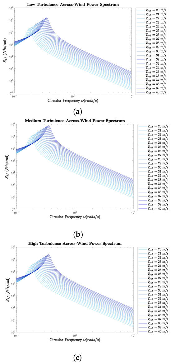
Figure 3.
Across-wind power spectra. (a) Low turbulence intensity. (b) Medium turbulence intensity. (c) High turbulence intensity.

Figure 4.
Comparison of across-wind power spectrum at = 40 m/s.
2.1. Response Model
To model the structure’s response, the spectral method of modal analysis is utilized, with analysis of the structure completed in the frequency domain. The displacement response spectrum can be obtained directly from the power spectrum of the wind forces by solving
The transfer function matrix used in the frequency-domain spectral analysis is computed directly in physical coordinates using the full coupled system matrices. For each frequency , the transfer matrix is is calculated as
This represents a full system (non-modal) transfer function. denote the mass, stiffness, and damping matrices, respectively. The acceleration response spectrum is obtainable from the displacement response spectrum through the following relationship:
The root mean squared (RMS) structural responses are available through the computation of the following quantities:
where and are vectors that contain the floor-wise RMS acceleration and displacements, respectively. The peak acceleration response is then estimated using a standard gust factor approach [47] such that
where the gust factor is given as
where is the fundamental natural frequency of the benchmark structure. represents the sampling time and is assumed to be 600 s. This spectral response model is used for all the structural arrangements considered. With each structural arrangement modeled through modification of the mass, stiffness, and damping matrices, these modifications are discussed below.
2.2. Uncontrolled Case
The uncontrolled case represents the benchmark structure’s response without any control device installed. The mass and stiffness matrix for the uncontrolled structure are notated as and , both . The damping matrix is developed using the Rayleigh damping method. The method is based on the identification of two variables and that are used in conjunction with the mass and stiffness matrices to develop the damping matrix. To this end, the damping matrix is a linear combination of the mass and stiffness matrices such that
where the dimensionless coefficients and are determined based on the desired damping ratios through the following matrix operation:
where and are the natural circular frequencies of the ith and jth modes in rad/s. and are the desired damping ratios (given in %) between the ith and jth modes.
The selection of damping ratios in this study follows the probabilistic framework introduced by Bashor et al. [48], which provides empirically derived damping ratios () for tall buildings subjected to wind loading. This framework accounts for inherent variability in structural damping and offers a realistic representation of damping effects in serviceability conditions.
Specifically, Bashor et al. [48] proposes a lognormal distribution of damping ratios (with a mean of 1 and a covariance of ) based on full-scale measurements of tall buildings. The stochasticity in the model is introduced through these empirically derived () values.
2.3. Control with a Tuned Mass Damper
The properties of the tuned mass damper (TMD) are modeled by appending an additional row and column to the uncontrolled system matrices, resulting in a 77 DOF structural model. The TMD is assumed to be located at the top floor of the structure and as such all modifications to the system matrices occur in the last two rows and columns. The TMD is tuned to the building’s fundamental natural frequency using the formulae proposed in [49] and given below.
where and are the tuning ratio and damping ratio of the TMD, respectively. denotes the ratio between the mass of the damper and the fundamental modal mass of the building, and it is taken as . These parameters are then used to generate the combined TMD system matrices, denoted as , , and , all , through the following matrix operations:
where is the fundamental modal mass of the building. The notation refers to the indices for assignment in the resultant matrices, where the comma delineates the row and column indices and the : operation notes the span in vector space of the assignment.
2.4. Control with a Tuned Mass Damper Fluid Inerter
Modifying the uncontrolled system matrices to include a Tuned Mass Damper Fluid Inerter (TMDFI) is not as straightforward as the inclusion of a TMD. First, the optimal TMDFI parameters must be selected, and then the inertance force must be linearized to allow for analysis in the frequency domain.
For a view of the mechanical diagram of the proposed TMDFI system, refer to Figure 5 below.
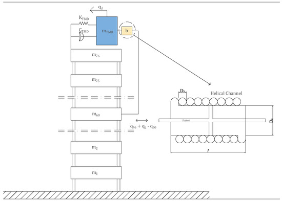
Figure 5.
Mechanical diagram of TMDFI system, adapted from [35].
The TMDFI parameters employed in this study are provided in Table 3; these are optimal TMDFI parameters. The inertance force depends on the selected TMDFI parameters, as shown in Table 3. Optimal tuning of the TMDFI is achieved by adjusting the tuning ratio and diameter ratio of the fluid inerter element. In this study, an optimization procedure is employed to minimize the variance in the structure’s modal displacements under white noise excitation , following the approach in [35]. The procedure uses the variance of the modal displacements as the cost function , with the optimization problem taking the general form of
where is the first component of the transfer matrix and . Using an analytical technique as per [50], the integral in Equation (24) can be obtained as
where , and . represents the equivalent damping ratio for the TMDFI system and is defined as
where , is the natural frequency of the building in rad/s, is the natural frequency of the damper in rad/s, the tuning ratio is defined as the ratio between and , and is the normalized displacement ratio between the top of the building and the height of the inerter hook from ground level determined as .
Table 3.
TMDFI parameters used.
Considering Equation (24), the constraint variables, I and u are vectors (, which are arbitrarily taken as and . This gives a solution to the optimization problem of for the benchmark problem considered. For further information on the optimization procedure and the arbitrary selection of I and u, readers should refer to [35].
Although this study is primarily concerned with building acceleration, the above optimization approach (minimization of the frequency-weighted modal displacement response of the augmented system) is sought as, follows:
- Displacement and acceleration responses are strongly correlated in lightly damped structures like the 76-story benchmark building, especially near the fundamental mode, which dominates the response.
- Acceleration is proportional to the second derivative of displacement; hence, improvements in displacement generally lead to improvements in acceleration response.
- Optimization based directly on acceleration spectra is also tested but found to be less stable numerically due to higher sensitivity to high-frequency components and noise in the power spectral density functions.
Once the optimal TMDFI parameters are identified, the inertance force is linearized to account for deviations from the ideal inerter device. These deviations arise from non-linear control forces generated by the TMDFI. A statistical linearization technique is used to linearize the non-linear damping force. The linearized damping coefficient is given as
where is the variance of the relative velocity between the inerter terminals. represents the non-linear damping inerter damping coefficient. In Equations (27) and (28), the standard deviation of the relative displacements at DOF is unknown and depends on the damping coefficient . It is observed in Equation (27) that a one-step solution is not possible, and therefore an iterative approach is utilized. By assuming an initial value of , an approximation of is determined. This approximated value is then used to generate a better estimate of in the next iteration. This iterative approach is taken until the values of and converge. The model assumes that convergence has occurred when the absolute difference between the values is less than .
With both the optimal TMDFI parameters identified and the non-linear damping force linearized, the TMDFI system matrices can be constructed. Similar to the TMD, the combined system matrices are notated as , , and , all , generated based on the following matrix operations:
where denotes the index of the floor number to which the inerter hook is attached.
and are dependent on the input.
2.5. Monte Carlo Simulations
Numerical simulations are conducted for both uncontrolled and controlled models. Reliability assessment under each turbulence case, as presented in Table 2, is performed using a one-step Monte Carlo Simulation (MCS). This method estimates the probability of failure for each structural arrangement at a given reference wind velocity, based on the wind loading and response models described earlier. Stochastic damping ratios are generated for each MCS sample, and the output response is evaluated against an acceleration limit state. The limit state, defined by ISO 10137:2007 [51], represents the maximum allowable peak acceleration for an office building with a 1-year return period. For the benchmark structure with a fundamental frequency of 0.16 Hz, this limit is 0.1376 m/s2. In this paper, we examine limit states at , and of the prescribed ISO peak acceleration limit value, as outlined in Table 4.
Table 4.
Expanded Limit State Values.
In this study, 21 reference wind velocities are considered, uniformly distributed between 20 and 40 m/s. For each simulation, random samples of are generated. This is used to generate a realization of the uncertain damping matrix using the Rayleigh damping method. This realized damping matrix is then used to calculate the RMS acceleration, RMS displacement, and peak acceleration for the three structural arrangements. The calculated peak acceleration is then checked for exceedance under the five expanded limit states; see Table 4. The required number of Monte Carlo samples is validated by assessing the convergence of peak acceleration at a reference wind speed of 30 m/s and a turbulence intensity of . A total of 10,000 samples are evaluated, with the mean and standard error of the mean calculated at intervals from 50 to 10,000 samples. Results show minimal variation beyond 500 samples, so 500 samples are used for each wind speed. With 21 reference wind velocities, this results in 10,500 simulations per turbulence intensity, totaling 31,500 simulations across all cases. A flowchart of the model outlined above is given in Figure 6.
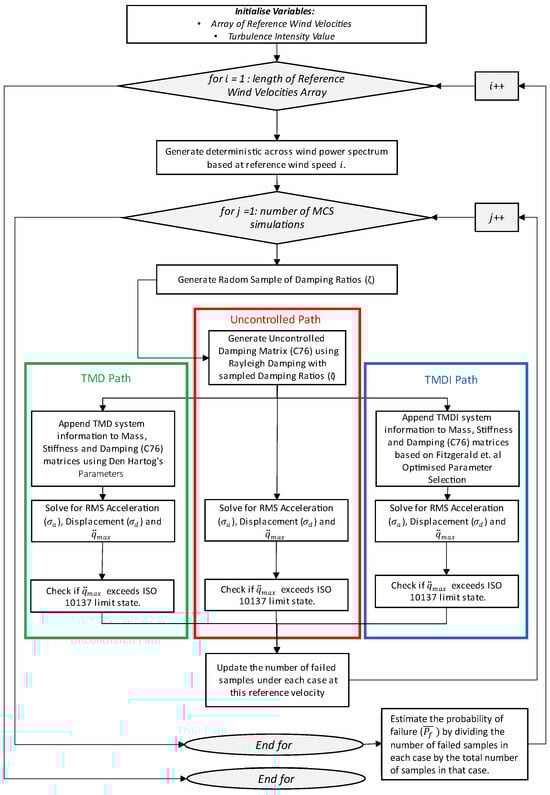
Figure 6.
Flow chart of model utilized [33,49].
3. Numerical Results
3.1. Acceleration Limit State and Fragility Curves
Fragility curves are used to graphically depict the progression of the probability of failure, , across the studied wind reference velocities and turbulence intensity levels. Each curve plots the probability of exceedance over the ISO acceleration limit against the reference velocity, resulting in nine fragility plots—one for each turbulence case (Figure 7). These curves show a complex relationship between and the reference velocity, observed as inflection points across the five expanded limit states. These inflections arise due to the discretization of 21 sampled reference velocities, with Piecewise Cubic Hermite interpolation used to generate smooth curves. This method preserves zero-probability values at consecutive intervals and ensures that does not exceed a value of one, offering a smoother alternative to linear interpolation. The inflection points are primarily due to the initial 1 m/s discretization. While the spectral method of analysis is computationally efficient, there is a trade-off between increasing the Monte Carlo Simulation (MCS) resolution at each reference velocity and increasing the number of velocity samples, both of which extend computation time.

Figure 7.
Acceleration fragility curves. (a) Low turbulence acceleration fragility curves. (b) Medium turbulence acceleration fragility curves. (c) High turbulence acceleration fragility curves.
In Figure 7, it is observed that the reference velocity required to exceed the five limit states decreases (in all cases) with increasing turbulence intensity. This is the expected result as it is observed that the total power of the across-wind power spectrum increases with turbulence intensity. The fragility curves shift to the left with increasing turbulence intensity. To assign magnitudes to this shift, the reference velocity at which >95% of the MCS samples exceed the A3 (ISO 10137 [51]) limit state are compared, with this comparison tabulated in Table 5.
Table 5.
Reference Wind Velocity Required for 95% of Samples to Fail at the A3 Limit State.
Additionally, it is evident that the TMDFI increases the reference velocity required for a 95% failure of the A3 limit state in all turbulence cases. Notably, this increase gives the TMDFI controlled structure similar performance to the uncontrolled structure but at reference velocities of 6–7 m/s higher. The TMDFI also offered 3–4 m/s of additional reference velocity before significant failure compared to the TMD-controlled structure. This represents an improvement in reliability for the TMDFI compared to the two other structural arrangements.
3.2. Peak Acceleration Response
To understand the improvement in reliability at the A3 limit state, the peak top-floor acceleration at each reference velocity is analyzed. Figure 8 shows the mean and standard error of peak acceleration for each structural arrangement under low, medium, and high turbulence. The mean peak accelerations from the MCS samples for the TMDFI and TMD are compared to the uncontrolled structure, with the percentage improvement in mean acceleration for each control scheme presented at each reference velocity.

Figure 8.
Magnitude of acceleration response. (a) Low turbulence. (b) Medium turbulence. (c) High turbulence.
Figure 8 shows that the TMDFI consistently outperforms the TMD in reducing peak acceleration across all turbulence cases. However, the percentage of improvement decreases with increasing wind speed for both control systems. This decline is not uniform, with the TMDFI experiencing a more pronounced drop in performance, particularly at higher turbulence intensities. The magnitude of this degradation is detailed in Table 6, where the TMDFI shows greater sensitivity to increased turbulence.
Table 6.
Comparison of Percentage Improvement in Peak Acceleration for Each Structural Arrangement.
Aggregating the results across all reference velocities, the TMDFI shows a 60.8% improvement over the uncontrolled structure and 28.9% over the TMD.
3.3. RMS Displacement Response
The RMS displacement response values were recorded to evaluate the performance differences between the acceleration and displacement responses of the control devices. Similar to the peak acceleration, Figure 9 presents the mean and standard error of the mean for the RMS displacement response across low-, medium-, and high-turbulence cases.
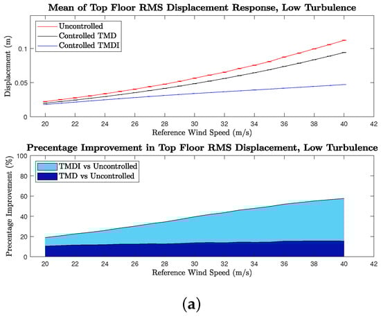
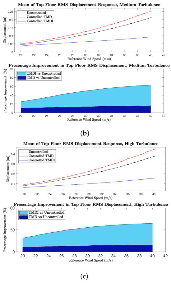
Figure 9.
Magnitude of RMS displacement response. (a) Low turbulence. (b) Medium turbulence. (c) High turbulence.
The plots reveal a notable relative improvement in the RMS displacement response for both the TMD and TMDFI across the sampled reference wind velocities. Specifically, the relative RMS displacement of the TMDFI improves with increasing reference velocity in all turbulence cases. These improvements are detailed in Table 7, with comparisons made at 20 m/s and 40 m/s, representing the minimum and maximum mean RMS displacement values recorded. The TMDFI shows a significant enhancement in RMS displacement, outperforming the TMD by 8.4% to 20.4% at 20 m/s and by 42.1% to 49.3% at 40 m/s.
Table 7.
Comparison of Percentage Improvement in the Mean RMS Displacement Response.
3.4. Contrasts Between the Displacement and Acceleration Response
This improvement in the displacement response contrasts with the degradation in performance of to when considering the TMDFI against the TMD in the peak acceleration response (Table 6). This disparity, with degradation in the peak acceleration whilst improvement in the RMS displacement response, can largely be attributed to two factors.
3.4.1. Optimization Procedure Used
This study optimizes for minimized modal displacements, resulting in TMDFI parameters that emphasize displacement response over acceleration. The observed 33% to 38% improvement in TMDFI displacement response as wind speed increases from 20 m/s to 40 m/s is not solely attributable to this bias. Rather, it likely arises from increased power in the across-wind spectrum, which amplifies modal displacements and relative floor accelerations, thereby enhancing TMDFI performance through greater inertance force. At lower speeds, the across-wind spectrum generates insufficient motion for high inertance forces, resulting in comparable performance between TMD and TMDFI. As wind velocity and turbulence intensify, higher terminal floor accelerations improve TMDFI effectiveness via increased inertance. Consequently, the acceleration between floors, driven by enhanced across-wind power, correlates with the improved TMDFI displacement response. However, this relationship does not fully account for the observed divergence between improved RMS displacement and the decline in peak acceleration response with increasing velocity.
3.4.2. Differences in the Response Spectra
Figure 10 provides a direct comparison of these spectra, displaying the maximum values from all 10,500 samples in the low-turbulence case at each circular frequency within the studied frequency band. The first three natural circular frequencies are denoted as , , and . Notably, the area under these curves is directly related to the RMS and peak responses.

Figure 10.
Comparison of the maximum response in displacement and acceleration spectra.
Figure 10 illustrates that the TMDFI significantly reduces the displacement response, particularly near the fundamental natural frequency. It also shows that higher-order natural frequencies ( and ) have a greater impact on the overall acceleration response than on the displacement response, evidenced by a steeper decline in the displacement spectra beyond the fundamental frequency. To assess the effect of increasing reference velocity, response spectra for both control arrangements were generated using deterministic damping parameters in the low-turbulence case, as depicted in Figure 11. Three key observations emerge: (1) the influence of the 2nd and 3rd modes increases with reference speed in both response spectra; (2) TMDFI and TMD most effectively reduce response spectra near the fundamental frequency; and (3) the effect of higher natural frequencies is more pronounced in the acceleration response. These findings elucidate the improved RMS displacement response alongside the degradation in peak acceleration response with rising reference velocity. While both control devices diminish response around the fundamental frequency, increased responses at higher frequencies lead to overall acceleration performance degradation. Conversely, the reduced influence of the 2nd and 3rd frequencies facilitates an overall improvement in displacement as reductions at the fundamental frequency prevail. These trends are consistent across medium- and high-turbulence cases, with deterministic response plots presented in Figure 12.

Figure 11.
Low-turbulence response spectra with mean damping parameters . Darker colors represent increasing cases.

Figure 12.
Low-turbulence response spectra with mean damping parameters . Blue = low turbulence, red = medium turbulence, green = high turbulence. Darker colors represent increasing cases.
3.5. System Uncertainty
We established a deterministic explanation for the disparity between displacement and acceleration responses and now investigate the influence of uncertain damping ratios. To evaluate this, we analyze the frequency band to identify conditions that produce the largest response variations. For each structural arrangement, we record the maximum and minimum response values at each frequency across all reference velocities and turbulence cases. For each sampled pair of damping ratios, the response is updated if it exceeds the previous maximum or falls below the previous minimum. This process, applied to all 10,500 samples per turbulence case, yields bounded maximum and minimum response plots.
As illustrated in Figure 13 for medium turbulence intensity, uncertain damping parameters introduce variability primarily in two regions of the response spectra: the background response zone (frequencies below the fundamental frequency) and around the natural frequencies, especially in the uncontrolled case. The controlled configurations (TMD and TMDI) show minimal variation (approximately ) at resonant frequencies, indicating effective response stabilization. Conversely, damping uncertainties in the uncontrolled case significantly influence whether the resonant response exceeds the background response, as evidenced by greater variability and a higher standard error of the mean.

Figure 13.
Minimum and maximum of acceleration and displacement response, medium turbulence. (a) Low turbulence. (b) Medium turbulence.
3.6. Influence of Turbulence Intensity
Increasing turbulence intensity leads to larger fluctuating force components and thus increases the energy content across the frequency domain. In contrast, increasing wind velocity primarily affects the mean structural response by scaling the steady aerodynamic forces while also shifting the frequency content of the PSD. Our parametric study, which considers a range of wind velocities (20–40 m/s) and three turbulence intensity levels (low, medium, and high), demonstrates that while wind velocity dictates the overall load magnitude, turbulence intensity has a dominant effect on peak structural responses, particularly for accelerations.
3.7. Limitations of Study
This study employs a frequency domain analysis to efficiently evaluate structural responses under wind excitation. This approach significantly enhances computational efficiency and enables a broad parametric investigation. However, it inherently provides response statistics—such as peak acceleration and displacement—derived from spectral integration rather than instantaneous time-domain responses. While this is a standard and widely accepted method in wind engineering, it does mean that peak accelerations are estimated using a gust factor approach, and displacement comparisons are based on root mean square values rather than direct time histories.
In addition, the Monte Carlo Simulation (MCS) framework used to evaluate probabilistic response characteristics adopts a uniform sample density across all reference wind velocities. This ensures consistency in the analysis but may be less efficient in cases where the probability of exceedance is very low. In such cases, a more adaptive sampling strategy could provide more refined probability estimates, albeit at a higher computational cost. Given the range of turbulence intensities and damping uncertainties considered, we do not expect this to significantly impact the overall findings, but it is an avenue for future refinement.
The current study represents an analytical framework to evaluate the reliability of a TMDI system. Further investigation and experimental work are required to assess the applicability of the proposed framework with regard to real scenarios.
3.8. Applicability to the Analysis and Reliability Evaluation of Tall Buildings
The method proposed in this study offers an attractive approach for designers of tall buildings in real scenarios. The benefits to engineers and designers are given below.
- The method outlined in this work can be readily implemented to a structural analysis process, and it requires only a structures geometric information and reduced mass and stiffness matrices. With this information, the designer can quickly assess the relative performance of the inclusion of a TMD or TMDI against an uncontrolled option.
- The proposed method can be readily modified to include different wind load models.
- The use of fragility curves allows for the reliability analysis to be communicated graphically.
4. Conclusions
This study evaluated the reliability and performance of the Tuned Mass Damper Fluid Inerter (TMDFI) using a benchmark structure comparing it with a traditional tuned mass damper (TMD) and an uncontrolled case. A deterministic across-wind model assessed performance over wind velocities (20–40 m/s) and turbulence intensities, incorporating lognormally distributed damping ratios (, Cov = 0.3) via a one-step Monte Carlo Simulation (31,500 samples, 80 h CPU time).
Peak acceleration and RMS displacement were calculated for each damping realization. Fragility curves showed the TMDFI significantly outperformed both the uncontrolled structure and TMD, with the uncontrolled structure failing 95% of the time between 20 and 35 m/s, while the TMDFI only failed beyond 27 m/s. Increased turbulence reduced reliability in all cases, highlighting its critical effect.
The TMDFI reduced peak top-floor acceleration by 60.8%, compared to 28.9% for the TMD, maintaining superior performance despite some degradation at higher velocities and turbulence. In terms of RMS displacement, the TMDFI improved by 18.9% to 64.8% over the uncontrolled case, showing robust performance under varying conditions.
The study underscored the impact of uncertain damping ratios on structural response and demonstrated the TMDFI’s effectiveness in mitigating both acceleration and displacement, confirming its potential for enhancing structural reliability of tall buildings under dynamic wind loading.
The methodology proposed in this study offers and attractive method that can be readily implemented to the analysis of tall buildings in real scenarios.
Future work on this topic should focus on experimental validation of the proposed TMDFI system, and indeed other inerter-based dampers, to complement the current simulation-based findings. In particular, full-scale or real-time hybrid testing is envisioned to assess the dynamic performance of the damper under realistic wind loading conditions. Such studies will provide critical insight into device behavior, implementation challenges, and system robustness. In parallel, deployment of the TMDFI in a real structural setting, supported by structural health monitoring (SHM), would offer valuable data to evaluate long-term performance and inform future design practice. These experimental efforts are essential to advance the practical adoption of inerter-based damping systems in tall buildings.
Author Contributions
Conceptualization, C.M. and B.F.; Methodology, C.M. and B.F.; Software, C.M. and B.F.; Validation, B.F.; Formal analysis, C.M.; Investigation, C.M.; Writing—original draft, C.M.; Writing—review & editing, B.F.; Supervision, B.F. All authors have read and agreed to the published version of the manuscript.
Funding
This research received no external funding.
Data Availability Statement
The original contributions presented in the study are included in the article, further inquiries can be directed to the corresponding author.
Conflicts of Interest
Author Cáelán McEvoy was employed by the company Arup. The remaining author declares that the research was conducted in the absence of any commercial or financial relationships that could be construed as a potential conflict of interest.
Nomenclature
| Cross-sectional area of the cylinder | m2 | |
| Cross-sectional area of the helical channel | m2 | |
| Rayleigh damping coefficient | - | |
| Rayleigh damping coefficient | - | |
| B | Width of the structure | m |
| b | Inertance | kg |
| C | Damping | Ns/m |
| Root mean squared lift coefficient | - | |
| Damping matrix (tuned mass damper) | Ns/m | |
| Damping matrix (tuned mass damper fluid inerter) | Ns/m | |
| Across-wind spectral bandwidth coefficient | - | |
| Across-wind spectral bandwidth coefficient | - | |
| Damping matrix (uncontrolled structure) | Ns/m | |
| Tuned mass damper fluid inerter damping coefficient | - | |
| Linearized tuned mass damper fluid inerter damping coefficient | - | |
| D | Depth of structure | m |
| Fluid inerter channel diameter | m | |
| Fluid inerter helix diameter | m |
| Inertance force | N | |
| TMDFI hook floor | - | |
| Vortex shedding frequency | Hz | |
| Gust factor | - | |
| H | Height of building | m |
| Height of atmospheric boundary | m | |
| Turbulence intensity | - | |
| K | Stiffness | N/m |
| Stiffness matrix (tuned mass damper) | N/m | |
| Stiffness matrix (tuned mass damper fluid inerter) | N/m | |
| Stiffness matrix (uncontrolled structure) | N/m | |
| L | Characteristic length (Strouhal) | m |
| M | Mass | kg |
| Mean | - | |
| Mass matrix (tuned mass damper) | kg | |
| Mass matrix (tuned mass damper fluid inerter) | kg | |
| Mass Matrix (uncontrolled structure) | kg | |
| Damper spring stiffness | N/m | |
| Tuned mass weight | kg | |
| Mass of fluid in helical channel | kg | |
| Fundamental modal mass | kg | |
| N | Number of simulations | - |
| Number of failures in N simulations | - | |
| Number of turns in the helix | - | |
| Probability of failure | - | |
| Estimate of the probability of failure | - | |
| Relative acceleration between inerter terminals | m/s2 | |
| Peak acceleration | m/s2 | |
| R | Fluid inerter bent radius of helix | m |
| Reynolds number | - | |
| Coherence function of across-wind spectra | - | |
| Radius of the piston | m | |
| Inner radius of the cylinder | m | |
| Inner radius of the helical channel | m | |
| Radius of the helix | m | |
| S | Plan area | m2 |
| Across-wind power spectrum | N2 s/rad | |
| Acceleration spectrum | (m/s2)2/Hz | |
| Displacement spectrum | (m)2/Hz | |
| Intensity of white noise | - | |
| Strouhal number | - | |
| Turbulence intensity | - | |
| Sampling time | s | |
| Absolute acceleration of inerter terminals | m/s2 | |
| V | Wind velocity (generic) | m/s |
| Reference wind velocity | m/s | |
| z | Height above ground level | m |
| Terrain power law coefficient | - | |
| Reliability index | - | |
| First component of transfer matrix | - | |
| Coherence function decay coefficient | - | |
| Tuned mass damper damping ratio | - |
| Damping ratio of mode i | - | |
| Damping ratio of mode j | - | |
| Tuned mass damper fluid inerter equivalent damping ratio | - | |
| Length of helical channel | m | |
| Dynamic viscosity of the fluid at reference temperature | Pa s | |
| Density of air | kg/m3 | |
| Mass density of the fluid at reference temperature | kg/m3 | |
| Root mean squared acceleration response | m/s2 | |
| Root mean squared displacement response | m | |
| Variance of the mean | - | |
| Variance of the relative terminal accelerations | m/s2 | |
| Kinematic viscosity of the fluid at reference temperature | cSt | |
| Normalized displacement ratio | - | |
| Circular frequency in the studied bandwidth | rad/s | |
| Fundamental natural frequency of the building | rad/s | |
| Natural frequency of the tuned mass damper fluid inerter | rad/s | |
| Natural circular frequency of mode i | rad/s | |
| Natural circular frequency of mode j | rad/s | |
| Tuning ratio of tuned mass damper fluid inerter | - | |
| Tuning ratio of tuned mass dampe | - | |
| Vortex shedding frequency | rad/s |
References
- Kareem, A.; Kijewski, T.; Tamura, Y. Mitigation of motions of tall buildings with specific examples of recent applications. Wind. Struct. 1999, 2, 201–251. [Google Scholar] [CrossRef]
- Kareem, A.; Gurley, K. Damping in structures: Its evaluation and treatment of uncertainty. J. Wind. Eng. Ind. Aerodyn. 1996, 59, 131–157. [Google Scholar] [CrossRef]
- Fitzgerald, B.; Basu, B. A monitoring system for wind turbines subjected to combined seismic and turbulent aerodynamic loads. Struct. Monit. Maint. 2017, 4, 175–194. [Google Scholar]
- Baisthakur, S.; Pakrashi, V.; Bhattacharya, S.; Fitzgerald, B. Impact of Sources of Damping on the Fragility Estimates of Wind Turbine Towers. ASCE-ASME J. Risk Uncertain. Eng. Syst. Part B Mech. Eng. 2024, 10, 041202. [Google Scholar] [CrossRef]
- Moore, H.; Broderick, B.; Fitzgerald, B. Experimental and computational evaluation of modal identification techniques for structural damping estimation. In Proceedings of the E3S Web of Conferences, Marseille, France, 27 May–3 June 2022; Volume 347, p. 01008. [Google Scholar]
- Hickey, J.; Moore, H.; Broderick, B.; Fitzgerald, B. Structural damping estimation from live monitoring of a tall modular building. Struct. Des. Tall Spec. Build. 2024, 33, e2067. [Google Scholar] [CrossRef]
- Chu, S.; Soong, T.T.; Reinhorn, A.M. Active, Hybrid, and Semi-Active Structural Control: A Design and Implementation Handbook; Wiley: New York, NY, USA, 2005. [Google Scholar]
- Tarpø, M.; Georgakis, C.; Brandt, A.; Brincker, R. Experimental determination of structural damping of a full-scale building with and without tuned liquid dampers. Struct. Control Health Monit. 2021, 28, e2676. [Google Scholar] [CrossRef]
- Jafari, M.; Alipour, A. Methodologies to mitigate wind-induced vibration of tall buildings: A state-of-the-art review. J. Build. Eng. 2021, 33, 101582. [Google Scholar] [CrossRef]
- Xu, Y.L.; Kwok, K.; Samali, B. Control of wind-induced tall building vibration by tuned mass dampers. J. Wind. Eng. Ind. Aerodyn. 1992, 40, 1–32. [Google Scholar] [CrossRef]
- Khodaie, N. Vibration control of super-tall buildings using combination of tapering method and TMD system. J. Wind. Eng. Ind. Aerodyn. 2020, 196, 104031. [Google Scholar] [CrossRef]
- Hickey, J.; Broderick, B.; Fitzgerald, B.; Moore, H. Mitigation of wind induced accelerations in tall modular buildings. Structures 2022, 37, 576–587. [Google Scholar] [CrossRef]
- Elias, S.; Matsagar, V. Wind response control of tall buildings with a tuned mass damper. J. Build. Eng. 2018, 15, 51–60. [Google Scholar] [CrossRef]
- Moon, K.S. Vertically distributed multiple tuned mass dampers in tall buildings: Performance analysis and preliminary design. Struct. Des. Tall Spec. Build. 2010, 19, 347–366. [Google Scholar] [CrossRef]
- Tamura, Y.; Fujii, K.; Ohtsuki, T.; Wakahara, T.; Kohsaka, R. Effectiveness of tuned liquid dampers under wind excitation. Eng. Struct. 1995, 17, 609–621. [Google Scholar] [CrossRef]
- Konar, T.; Ghosh, A. A review on various configurations of the passive tuned liquid damper. J. Vib. Control 2023, 29, 1945–1980. [Google Scholar] [CrossRef]
- Khodaie, N. Parametric study of wind-induced vibration control of tall buildings using TMD and TLCD systems. Structures 2023, 57, 105126. [Google Scholar] [CrossRef]
- Kang, J.; Kim, H.S.; Lee, D.G. Mitigation of wind response of a tall building using semi-active tuned mass dampers. Struct. Des. Tall Spec. Build. 2011, 20, 552–565. [Google Scholar] [CrossRef]
- Zhu, W.; Luo, M.; Dong, L. Semi-active control of wind excited building structures using MR/ER dampers. Probabilistic Eng. Mech. 2004, 19, 279–285. [Google Scholar] [CrossRef]
- Qin, X.; Zhang, X.; Sheldon, C. Study on semi-active control of mega-sub controlled structure by MR damper subject to random wind loads. Earthq. Eng. Eng. Vib. 2008, 7, 285–294. [Google Scholar] [CrossRef]
- Ricciardelli, F.; Pizzimenti, A.D.; Mattei, M. Passive and active mass damper control of the response of tall buildings to wind gustiness. Eng. Struct. 2003, 25, 1199–1209. [Google Scholar] [CrossRef]
- Ümütlü, R.C.; Ozturk, H.; Bidikli, B. A robust adaptive control design for active tuned mass damper systems of multistory buildings. J. Vib. Control 2021, 27, 2765–2777. [Google Scholar] [CrossRef]
- Zhou, K.; Zhang, J.W.; Li, Q.S. Control performance of active tuned mass damper for mitigating wind-induced vibrations of a 600-m-tall skyscraper. J. Build. Eng. 2022, 45, 103646. [Google Scholar] [CrossRef]
- Cao, H.; Reinhorn, A.; Soong, T. Design of an active mass damper for a tall TV tower in Nanjing, China. Eng. Struct. 1998, 20, 134–143. [Google Scholar] [CrossRef]
- Kavyashree, B.; Patil, S.; Rao, V.S. Review on vibration control in tall buildings: From the perspective of devices and applications. Int. J. Dyn. Control 2021, 9, 1316–1331. [Google Scholar] [CrossRef]
- Kim, H.; Adeli, H. Wind-induced motion control of 76-story benchmark building using the hybrid damper-TLCD system. J. Struct. Eng. 2005, 131, 1794–1802. [Google Scholar] [CrossRef]
- Lu, X.; Zhang, Q.; Weng, D.; Zhou, Z.; Wang, S.; Mahin, S.A.; Ding, S.; Qian, F. Improving performance of a super tall building using a new eddy-current tuned mass damper. Struct. Control Health Monit. 2017, 24, e1882. [Google Scholar] [CrossRef]
- Liu, C.; Chen, L.; Lee, H.P.; Yang, Y.; Zhang, X. A review of the inerter and inerter-based vibration isolation: Theory, devices, and applications. J. Frankl. Inst. 2022, 359, 7677–7707. [Google Scholar] [CrossRef]
- Smith, M.C. Synthesis of mechanical networks: The inerter. In Proceedings of the 41st IEEE Conference on Decision and Control, Las Vegas, NV, USA, 10–13 December 2002; Volume 2, pp. 1657–1662. [Google Scholar]
- Giaralis, A.; Petrini, F. Wind-induced vibration mitigation in tall buildings using the tuned mass-damper-inerter. J. Struct. Eng. 2017, 143, 04017127. [Google Scholar] [CrossRef]
- Sarkar, S.; Fitzgerald, B. Vibration control of spar-type floating offshore wind turbine towers using a tuned mass-damper-inerter. Struct. Control Health Monit. 2020, 27, e2471. [Google Scholar] [CrossRef]
- Zhang, Z.; Fitzgerald, B. Tuned mass-damper-inerter (TMDI) for suppressing edgewise vibrations of wind turbine blades. Eng. Struct. 2020, 221, 110928. [Google Scholar] [CrossRef]
- Fitzgerald, B.; McAuliffe, J.; Baisthakur, S.; Sarkar, S. Enhancing the reliability of floating offshore wind turbine towers subjected to misaligned wind-wave loading using tuned mass damper inerters (TMDIs). Renew. Energy 2023, 211, 522–538. [Google Scholar] [CrossRef]
- De Domenico, D.; Deastra, P.; Ricciardi, G.; Sims, N.D.; Wagg, D.J. Novel fluid inerter based tuned mass dampers for optimised structural control of base-isolated buildings. J. Frankl. Inst. 2019, 356, 7626–7649. [Google Scholar] [CrossRef]
- Sarkar, S.; Fitzgerald, B. Design of Tuned Mass Damper Fluid Inerter for Wind-Induced Vibration Control of a Tall Building. J. Struct. Eng. 2024, 150, 04023242. [Google Scholar] [CrossRef]
- Sarkar, S.; Fitzgerald, B. Fluid inerter for optimal vibration control of floating offshore wind turbine towers. Eng. Struct. 2022, 266, 114558. [Google Scholar] [CrossRef]
- Swift, S.; Smith, M.C.; Glover, A.; Papageorgiou, C.; Gartner, B.; Houghton, N.E. Design and modelling of a fluid inerter. Int. J. Control 2013, 86, 2035–2051. [Google Scholar] [CrossRef]
- Giaralis, A.; Taflanidis, A. Optimal tuned mass-damper-inerter (TMDI) design for seismically excited MDOF structures with model uncertainties based on reliability criteria. Struct. Control Health Monit. 2018, 25, e2082. [Google Scholar] [CrossRef]
- Ruiz, R.; Taflanidis, A.; Giaralis, A.; Lopez-Garcia, D. Risk-informed optimization of the tuned mass-damper-inerter (TMDI) for the seismic protection of multi-storey building structures. Eng. Struct. 2018, 177, 836–850. [Google Scholar] [CrossRef]
- Petrini, F.; Giaralis, A.; Wang, Z. Optimal tuned mass-damper-inerter (TMDI) design in wind-excited tall buildings for occupants’ comfort serviceability performance and energy harvesting. Eng. Struct. 2020, 204, 109904. [Google Scholar] [CrossRef]
- Zhou, S.; Huang, J.; Yuan, Q.; Ma, D.; Peng, S.; Chesne, S. Optimal Design of Tuned Mass-Damper-Inerter for Structure with Uncertain-but-Bounded Parameter. Buildings 2022, 12, 781. [Google Scholar] [CrossRef]
- Peng, Y.; Sun, P. Reliability-based design optimization of tuned mass-damper-inerter for mitigating structural vibration. J. Sound Vib. 2024, 572, 118166. [Google Scholar] [CrossRef]
- Yang, J.N.; Agrawal, A.K.; Samali, B.; Wu, J.C. Benchmark problem for response control of wind-excited tall buildings. J. Eng. Mech. 2004, 130, 437–446. [Google Scholar] [CrossRef]
- Liang, S.; Liu, S.; Li, Q.; Zhang, L.; Gu, M. Mathematical model of acrosswind dynamic loads on rectangular tall buildings. J. Wind. Eng. Ind. Aerodyn. 2002, 90, 1757–1770. [Google Scholar] [CrossRef]
- Simiu, E.; Scanlan, R.H. Wind Effects on Structures: Fundamentals and Application to Design; John Willey & Sons Inc.: Hoboken, NJ, USA, 1996; p. 605. [Google Scholar]
- Gu, M.; Quan, Y. Across-wind loads of typical tall buildings. J. Wind. Eng. Ind. Aerodyn. 2004, 92, 1147–1165. [Google Scholar] [CrossRef]
- Davenport, A.G. Gust loading factors. J. Struct. Div. 1967, 93, 11–34. [Google Scholar] [CrossRef]
- Bashor, R.; Kijewski-Correa, T.; Kareem, A. On the wind-induced response of tall buildings: The effect of uncertainties in dynamic properties and human comfort thresholds. In Proceedings of the Americas Conference on Wind Engineering, Baton Rouge, LA, USA, 31 May–4 June 2005; Volume 31. [Google Scholar]
- Hartog, D. Mechanical Vibrations; McGraw-Hill Book Company, Inc.: New York, NY, USA, 1956. [Google Scholar]
- Roberts, J.B.; Spanos, P.D. Random Vibration and Statistical Linearization; Courier Corporation: North Chelmsford, MA, USA, 2003. [Google Scholar]
- ISO 10137:2007; Bases for Design of Structures–Serviceability of Buildings and Walkways Against Vibrations. International Organization for Standardization (ISO): Geneva, Switzerland, 2007.
Disclaimer/Publisher’s Note: The statements, opinions and data contained in all publications are solely those of the individual author(s) and contributor(s) and not of MDPI and/or the editor(s). MDPI and/or the editor(s) disclaim responsibility for any injury to people or property resulting from any ideas, methods, instructions or products referred to in the content. |
© 2025 by the authors. Licensee MDPI, Basel, Switzerland. This article is an open access article distributed under the terms and conditions of the Creative Commons Attribution (CC BY) license (https://creativecommons.org/licenses/by/4.0/).