Article

Unsteady Numerical Simulation of Two-Dimensional Airflow over a Square Cross-Section at High Reynolds Numbers as a Reduced Model of Wind Actions on Buildings

by
Aggelos C. Karvelis
1,
Athanassios A. Dimas
2 and
Charis J. Gantes
1,*
1
Institute of Steel Structures, National Technical University of Athens, GR-15780 Athens, Greece
2
Hydraulic Engineering Laboratory, Department of Civil Engineering, University of Patras, GR-26504 Rio, Greece
*
Author to whom correspondence should be addressed.
Buildings 2024, 14(3), 561; https://doi.org/10.3390/buildings14030561
Submission received: 3 January 2024 / Revised: 12 February 2024 / Accepted: 15 February 2024 / Published: 20 February 2024

Abstract

Airflow over a square cross-section at high Reynolds numbers and different angles of incidence is investigated with the aim of providing deeper insight into wind actions on elongated structures and, in particular, tall buildings. The flow around bluff bodies is characterized by separation at sharp corners, as well as possible flow reattachment at side surfaces. The alternate shedding of vortices is also generated in the wake of bluff bodies due to the unsteady nature of flow separation. Two-dimensional (2D) URANS numerical simulations were conducted in order to model transient flow and examine wind actions on a square used as a model of a typical cross-section of a tall building far from its roof and the ground. For validation purposes, the study’s numerical results on drag and lift coefficients, Strouhal numbers, as well as pressure coefficient distribution were found to be in good agreement with available experimental and numerical results in the literature for relatively low Reynolds numbers. The numerical study was then extended to higher Reynolds numbers, approaching values that are pertinent for wind flow around buildings, thus addressing the lack of such results in the literature. On the basis of these results, the impact of Reynolds numbers and angles of incidence on drag and lift coefficients, as well as the pressure coefficient distribution along the walls of the cross-section, is highlighted.

1. Introduction

The response of elongated structures and, in particular, tall buildings to wind actions is an important aspect of their structural design and becomes critical as the height of buildings increases, considering that the wind intensity is gaining strength and the buildings are laterally more flexible. In order to assess the effects of wind on buildings, a realistic estimation of the developing wind pressures and resultant loads is necessary.
Systematic engineering methods to that effect are largely founded upon the pioneering work on quasi-static wind loads by Cook, Harris, and their co-workers in the 1980s [1,2,3,4]. Kwok (1982) identified that for tall buildings, the cross-wind response may be of high importance for their structural stability [5], while Wacker and Plate (1993) proposed gust factors and peak wind pressure coefficients for cuboidal buildings [6]. Aerodynamic effects have been discussed by Zhou (2003) and various others [7].
Overviews of wind loading on structures have been published in several textbooks, such as ones by Stathopoulos and Baniotopoulos (2007) [8] and Holmes (2007) [9]. Petrini and Ciampoli (2012) proposed employing performance-based designs of tall buildings against wind, in a similar manner as for seismic designs [10]. With the advancement of computational tools, extensive efforts to address wind designs by means of advanced numerical analyses have been published in recent years [11,12,13,14]. Moreover, wind pressure distributions have also been proposed for various types of structures other than buildings, such as wind turbines [15] and solar collectors [16].
In terms of wind forcing, the cross-sections of elongated structures are characterized as bluff bodies, which are subjected to aerodynamic processes, such as flow stagnation, flow separation, and vortex shedding. In this paper, the two-dimensional (2D) airflow around a square, representing a horizontal cross-section of a building, is studied. A typical building with a square plan view of dimensions D by D and height h is shown in Figure 1. The aspect ratio of the square cylinder is defined as AR = h/D and is a critical parameter of wind responses. Excluding the lower part of the building, where boundary layer effects due to the ground are significant, as well as the upper part where flow separation occurs, wind flow in the intermediate part resembles 2D conditions and may be approximated using the proposed approach.
For buildings with a square cross-section and AR ≤ 5, the computation is based on the distribution of a pressure coefficient, cp, along the surfaces of the cross-section, defined as the following:
c p = p p 0.5 ρ U 2
where p is the pressure on the walls of the cross-section, p is the pressure in the freestream, ρ = 1.225 kg/m3 is the density of air, and U is the free-stream velocity. For buildings with a square cross-section and AR > 5, the computation is based on the force (drag) coefficient, cf, per unit height of the building, defined as the following:
c f = F w 0.5 ρ U 2 D
where Fw is the wind force per unit height. The Reynolds number of the corresponding airflow is defined as the following:
R e = ρ U D μ
where μ = 1.8 × 10⁻⁵ kg/m × s is the dynamic viscosity of air. For a bluff body, like the square cross-section considered here, alternating vortex shedding occurs in the wake of the body, and it is characterized by the dimensionless Strouhal number, defined as the following:
S t = f D U
where f is the frequency of vortex shedding.
Typical Re values for building applications are larger than 106, for which very limited results are available in the literature. Experiments have been conducted by many researchers to study airflow over very long (AR >> 5) square or rectangular cylinders. Delany and Sorensen (1953) [17] measured drag coefficients and St values for a wide range of Re values and for various shapes of bluff bodies, and they demonstrated the effect of rounded corners to the aerodynamic behavior. They showed that the drag coefficient remains stable over a wide range of Re values from 104 to 2 × 10⁶, although most experiments they performed were for Reynolds numbers ranging between 104 and 105. Vickery (1966) [18] presented the differences of fluctuating lift and drag coefficients for laminar and turbulent flow conditions. Lee (1975) [19] showed that the maximum value of St occurs at the angle of incidence, for which the drag coefficient has its minimum value. The pressure distribution on a square cross-section was investigated by Bearman and Obasaju (1982) [20] at Re = 2.2 × 10⁴. Igarashi (1984) [21] performed experiments at 3.85 × 10³Re ≤ 7.7 × 10⁴ in order to investigate the characteristics of the flow at angles of incidence between 0° and 45°. They determined four flow patterns and showed the existence of correlations between vortex shedding frequency and pressure distribution for each flow pattern.
Knisely (1990) [22] examined the St values for rectangular cylinders with plan view side ratios ranging from 0.04 to 1. Norberg (1993) [23] carried out experiments at Re = 3 × 10⁴, for rectangular cylinders with side ratios ranging from 1 to 3 and angles of incidence between 0° and 90°. Luo et al. (1994) [24] examined the aerodynamic behavior of four cross-sectional shapes, including a square, two trapezoidals, and a triangle. They presented the effect of the angle of incidence and flow reattachment on the drag coefficient. The velocity field around a square cylinder in a closed water channel was measured by Lyn et al. [25] using laser–Doppler velocimetry (LDV) at Re = 2.14 × 10⁴. Tamura and Miyagi (1999) [26] experimentally determined that the increase in turbulence intensity and the corner modification resulted in a reduction in drag forces. Van Oudheusden et al. (2008) [27] examined the flow field around a square cylinder at Re = 4 × 10³, 104, and 2 × 10⁴. They observed some effect at the separation region, while no differences were found on the mean flow for the examined Re numbers. Carassale et al. (2014) [28] experimentally examined the effect of rounded corners on the aerodynamic behavior of a square cylinder at 1.7 × 10⁴Re ≤ 2.3 × 10⁵ and angles of incidence between 0° and 45°. Finally, van Hinsberg et al. (2017) [29] also examined the effect of rounded corners on the aerodynamic behavior of a square cylinder at Re up to 12 × 106 and three angles of incidence (0°, 22.5°, and 45°).
Moreover, many researchers have numerically approached the airflow over a square cylinder. Sohankar (2006) [30] investigated cases at 103Re ≤ 5 × 10⁶ by performing large-eddy simulations (LESs) and showed that the mean drag coefficient is independent of the Reynolds number because flow separation occurs at the sharp leading edges of the body. Oka and Ishihara (2009) [31] examined the effect of the angle of incidence, between 0° and 45°, performing LESs at Re = 104. Xu et al. (2011) [32] performed unsteady Reynolds averaged Navier–Stokes (URANS) simulations at Re = 2.14 × 10⁴. For turbulence closure, they used several turbulence models, such as standard k-ε, renormalization group (RNG) k-ε, realizable k-ε, standard k-ω, shear stress transport (SST) k-ω, and Reynolds stress models (RSMs). Results with k-ω (SST) were found to agree the best with experimental results. Tian et al. (2013) [33] conducted URANS simulations using the k-ω (SST) turbulence model in order to investigate the flow around a rectangular cylinder at Re = 2.14 × 10⁴. The very good agreement of the numerical results with experimental data confirmed the validity of 2D URANS simulations for this Re and showed that the St is not sensitive to differentiation in the side ratio (d/b in Figure 1). Cao and Tamura (2016) [34] performed LESs with structured and unstructured grids at Re = 2.2 × 10⁴ and a zero-degrees angle of incidence. Zhang et al. (2017) [35] performed URANS simulations with Spalart–Allmaras (SA), standard k-ω, and k-ω (SST) turbulence models at Re = 2.2 × 10⁴, but observed that the one-equation Wray–Agarwal (WA) turbulence model agreed more with experimental data. Finally, Dai et al. (2017) [36] performed URANS simulations with the modified k-ε turbulence model, and they demonstrated the drag reduction effect of the presence of rounded corners instead of sharp ones in a square cylinder.
The objective of this study is to apply URANS to numerically examine the aerodynamic behavior of a square cross-section at high Reynolds numbers and several angles of incidence, as a model of a typical cross-section of a tall building (AR >> 5) far from its roof and the ground, in order to reveal the effect of Re on the drag and lift forces, as well as on the pressure distribution on the walls of the cross-section. It is noted that, according to ΕΝ1991-1-4 [37], the recommended value of the force (drag) coefficient is cf = 2.1 for a square cross-section, while the St value is 0.12 when AR > 5. The suggested value in the Australian Code AS/NZS [38] is cf = 2.2. From corresponding studies in the literature [39,40], it can be deduced that the force coefficient increases as the AR increases. Okamoto and Uemura (1991) [39] reported that for buildings with a square cross-section and sharp corners, the height-averaged force coefficient is cf = 1.3 for AR = 1 and cf = 2.2 for AR→∞, while McClean and Summer (2014) [40] obtained values of cf = 1.29 for AR = 3 and cf = 1.46 for AR = 11. Therefore, for tall buildings (AR >> 5), it is safe to consider that the 2D flow over a square is an appropriate model that can be used to compute the pressure distribution on the square cross-sections of the building, far from its roof and the ground, both as a standalone result and also a result to complement the single cf value provided by Eurocode 1.
The numerical model used here is based on URANS simulations of an unsteady turbulent flow using ANSYS Fluent [41]. The k-ω (SST) turbulence model was used for turbulence closure, while wall functions were used to model the boundary layer. The numerical simulations were conducted for Re = 2.2 × 10⁴ for validation purposes by comparing them to experimental and numerical data from the literature, and then for Re = 2 × 10⁶ and Re = 107, with the aim of simulating wind flow at realistic situations for buildings.

2. Materials and Methods

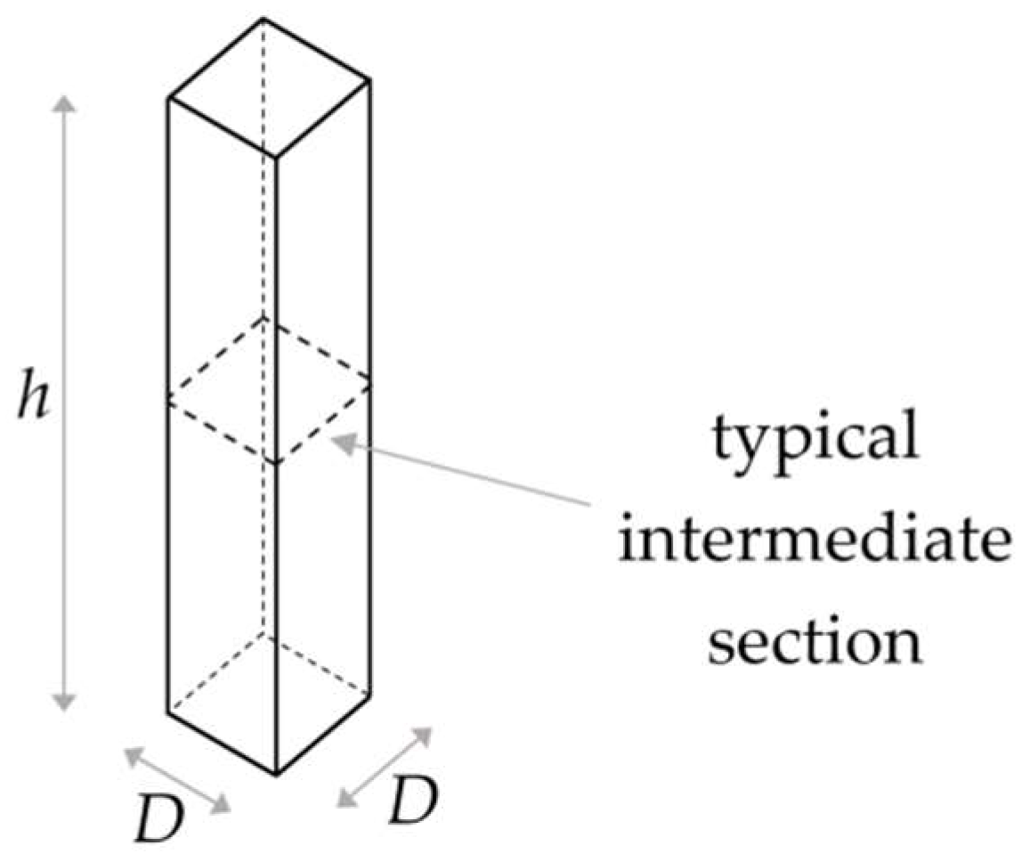
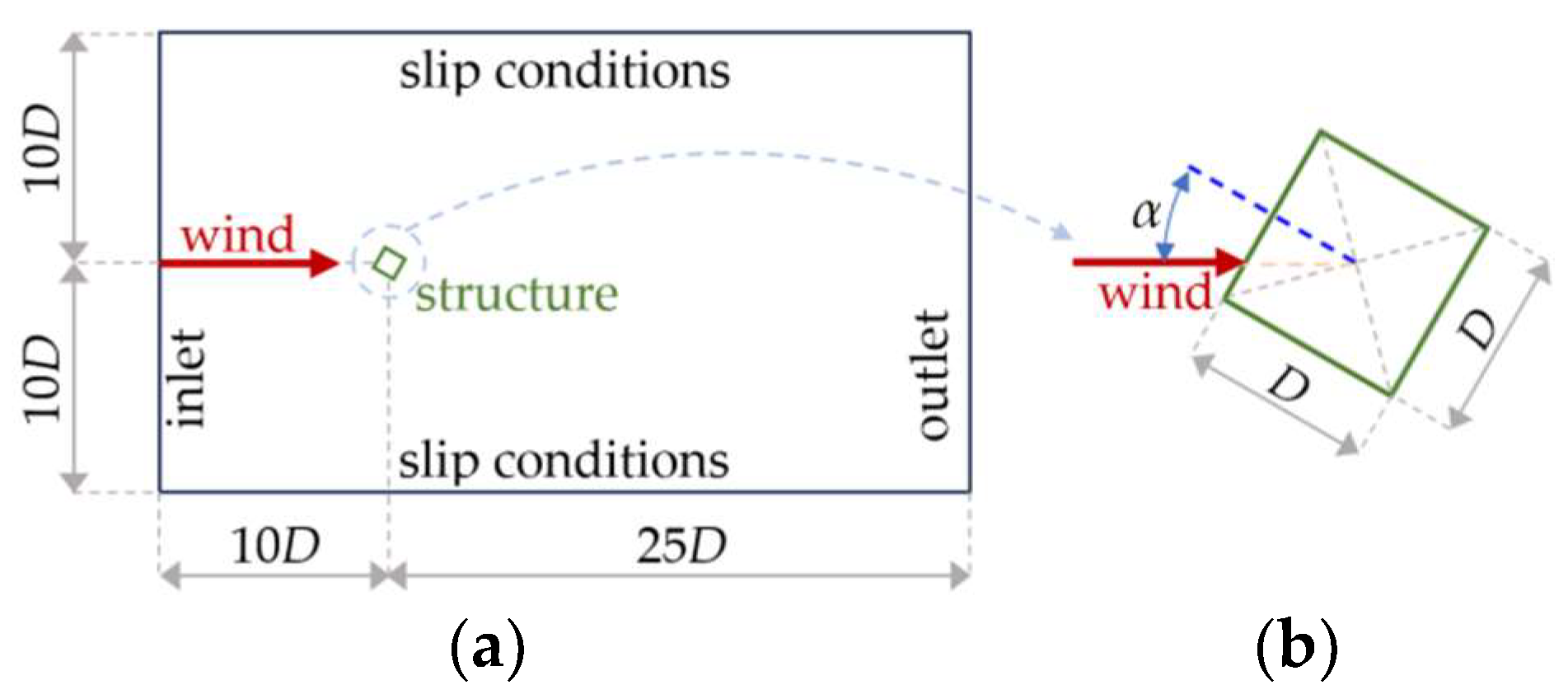
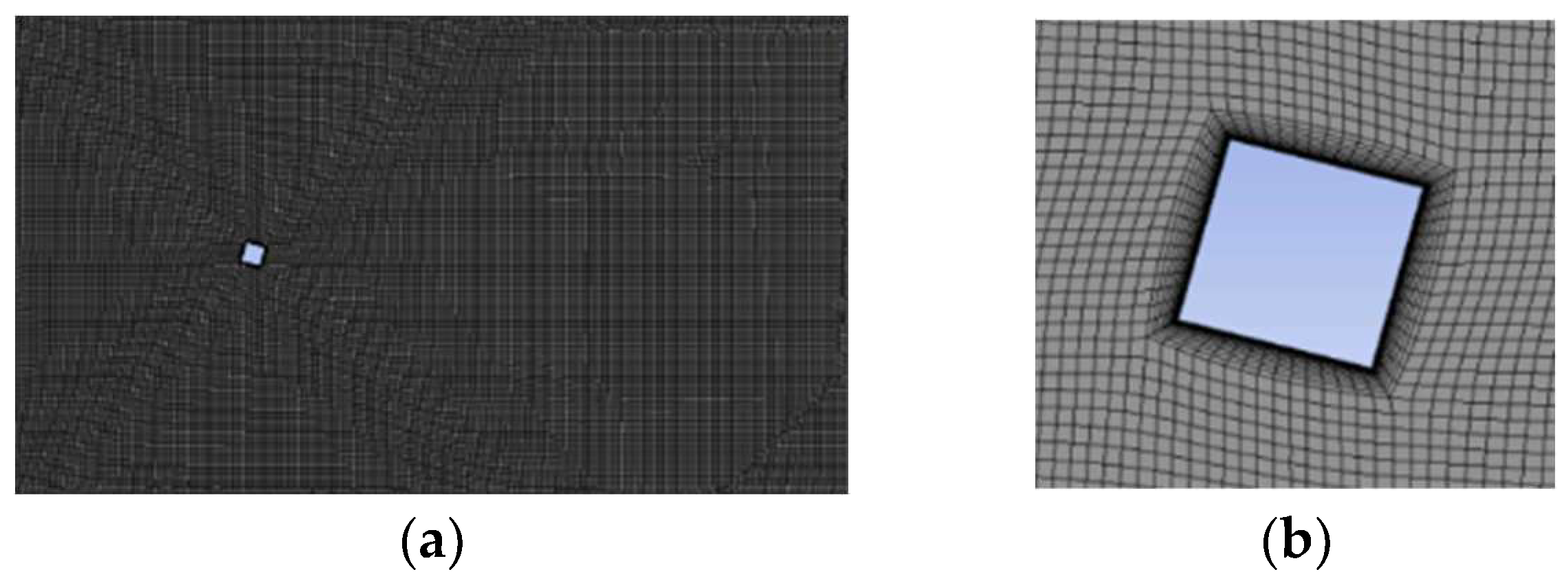
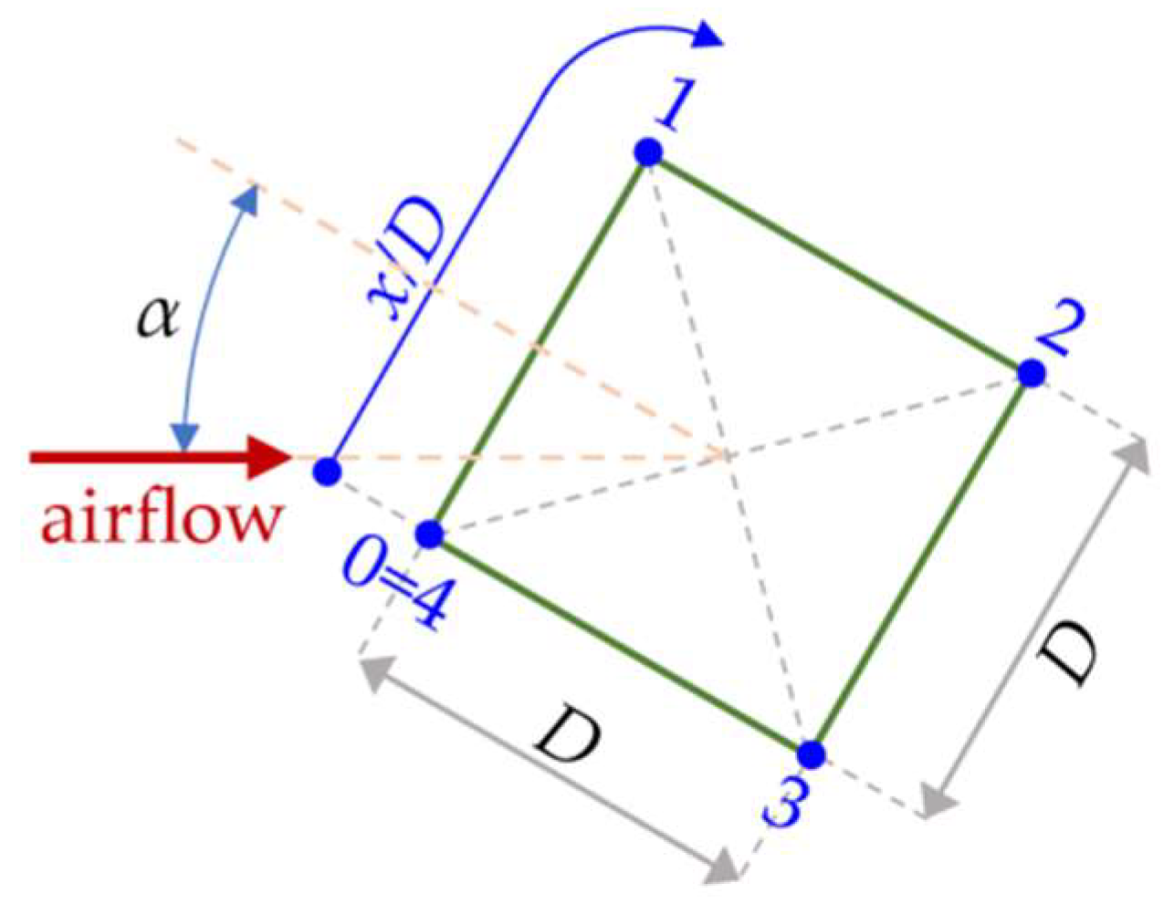
2.1. Computational Model

The aerodynamic behavior of a square cross-section with side D was numerically investigated by performing 2D URANS simulations. The computational fluid domain is shown in Figure 2a, where its dimensions are given in multiples of D. The inlet, outlet, and side boundaries of the computational domain are located at distances of 10D, 25D, and 10D, respectively, from the cross-section. The dimensions of the fluid domain were chosen so that flow development far from the cross-section was not affected and so that it could be comparable with previous numerical studies [32,33,36]. Initial analyses for varying D values confirmed that the results are independent of D; thus, this problem may be non-dimensionalized.
The airflow over the cross-section was investigated for several angle of incidence α values, as defined in Figure 2b. No slip conditions were applied on the cross-section walls. A uniform velocity profile was applied at the inlet boundary, the zero-velocity gradient was set at the outlet, and the slip conditions were imposed on the side boundaries of the computational domain. The turbulence intensity level of the incoming flow, I, is defined at the inlet boundary.
In ANSYS Fluent [41], the 2D incompressible URANS equations were solved using the finite volume method (FVM). Hybrid mesh was used to discretize the computational domain, as shown in Figure 3a. Details of the mesh around the bluff body are shown in Figure 3b. A grid independence study was carried out and it was concluded that a fluid domain consisting of 89,000 elements is adequate. The average heights of the first cell above the cross-section walls were 0.04D, 0.01D, and 0.0025D, while the corresponding dimensions in wall units were 35, 120, and 150 for Re = 2.2 × 10⁴, 2 × 10⁶, and 107, respectively, to facilitate the use of the standard wall function approach to model the boundary layers on the cross-section walls. An average cell size of 0.09D was used for discretization purposes in the rest of the computational domain. As already mentioned, the numerical study was initially conducted for Re = 2.2 × 10⁴ in order to validate the numerical model by comparing the experimental and numerical results from the literature, and then for 2 × 10⁶ and 107, which are representative of wind flow measurements for buildings.
For pressure–velocity coupling, the PISO algorithm was used because it was considered to be the most appropriate, among the available ones, to maintain a stable calculation in unsteady flows. Due to the use of a hybrid mesh and the presence of swirling flows, quadratic upwind interpolation was used as the interpolation scheme for the convection term. For the Reynolds stress term calculation, the eddy viscosity model k-ω (SST) [42,43] was used due to its strong performance in modeling flow separation cases [44]. The Courant number (Co) is defined as the following:
C o = U Δ x Δ t
where Δt is the time step and Δx is the average cell size. The time step (Δt) was chosen so that the Courant–Friedrichs–Lewy (CFL) condition, Co ≤ 0.1, was satisfied everywhere in the computational domain.

2.2. Aerodynamic Parameters

The aerodynamic parameters obtained by the simulations are summarized in this section. The instantaneous pressure coefficient, cp, on the walls of the square cross-section was computed, in line with Equation (1), and is a function of time. The corresponding mean pressure coefficient is defined as the following:
c p , m e a n = 1 N i = 1 N c p , i
while the corresponding rms pressure coefficient is defined as the following:
c p , r m s = 1 N i = 1 N ( c p , i c p , m e a n ) 2
where cp,i is the instantaneous pressure coefficient at time iΔt and N is the number of time samples. The instantaneous force coefficients of the cross-section, cf (drag in the streamwise direction) and cl (lift in the cross-wind direction), were computed according to Equation (2), where the force components were obtained by an appropriate integration of the wall pressure. The corresponding mean drag coefficient is defined as the following:
c f , m e a n = 1 N i = 1 N c f , i
and the corresponding rms drag coefficient is defined as the following:
c f , r m s = 1 N i = 1 N c f , i c f , m e a n
while the corresponding mean and rms lift coefficients are defined accordingly. In the following, the time series of the instantaneous aerodynamic coefficients is presented with respect to dimensionless time:
t * = t U D
where t is the time. The statistics of the above aerodynamic parameters were obtained over 25 vortex shedding cycles.
For design purposes, the extreme (max and min) wind pressure coefficients are computed as the following:
c p , max = c p , m e a n + k c p , r m s
c p , min = c p , m e a n k c p , r m s
where k is the peak factor, which correlates the max and min cp values to the rms ones. Two values of the peak factor, k = 2.5 and k = 3.5, were used here, taking into account the fact that in the literature, k values vary between 2.5 and 4.0 [45,46,47,48], while the value k = 3.5 is used in Eurocode 1 [37].

3. Results

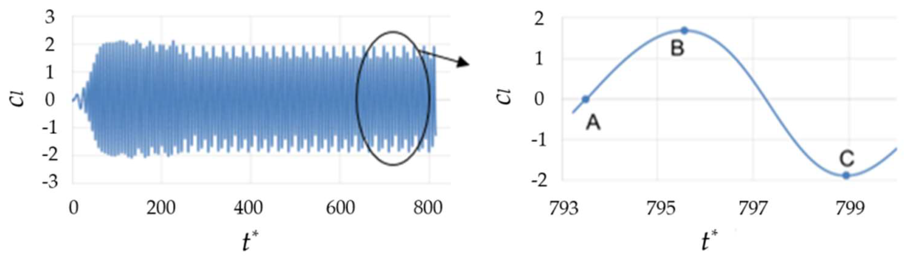
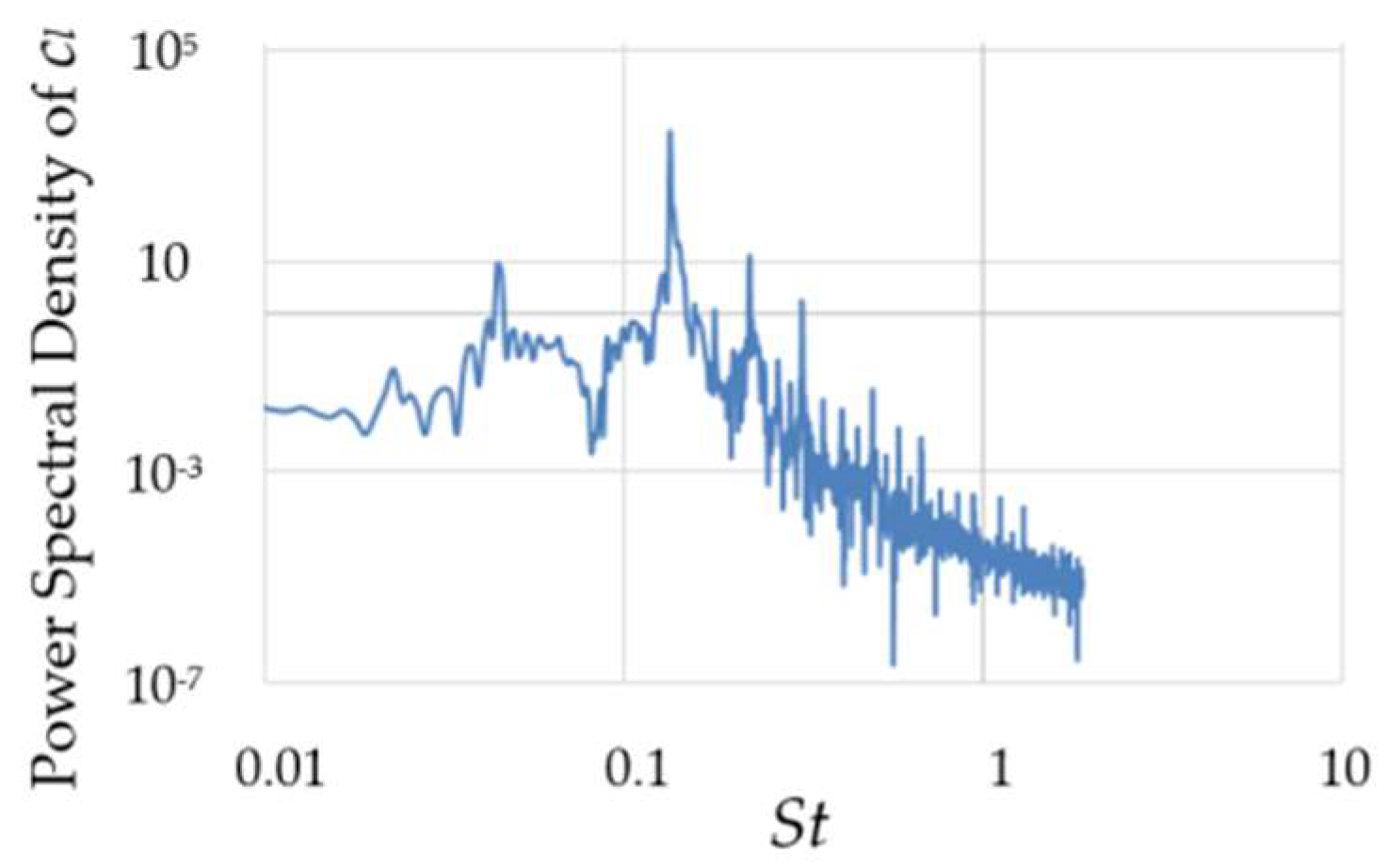
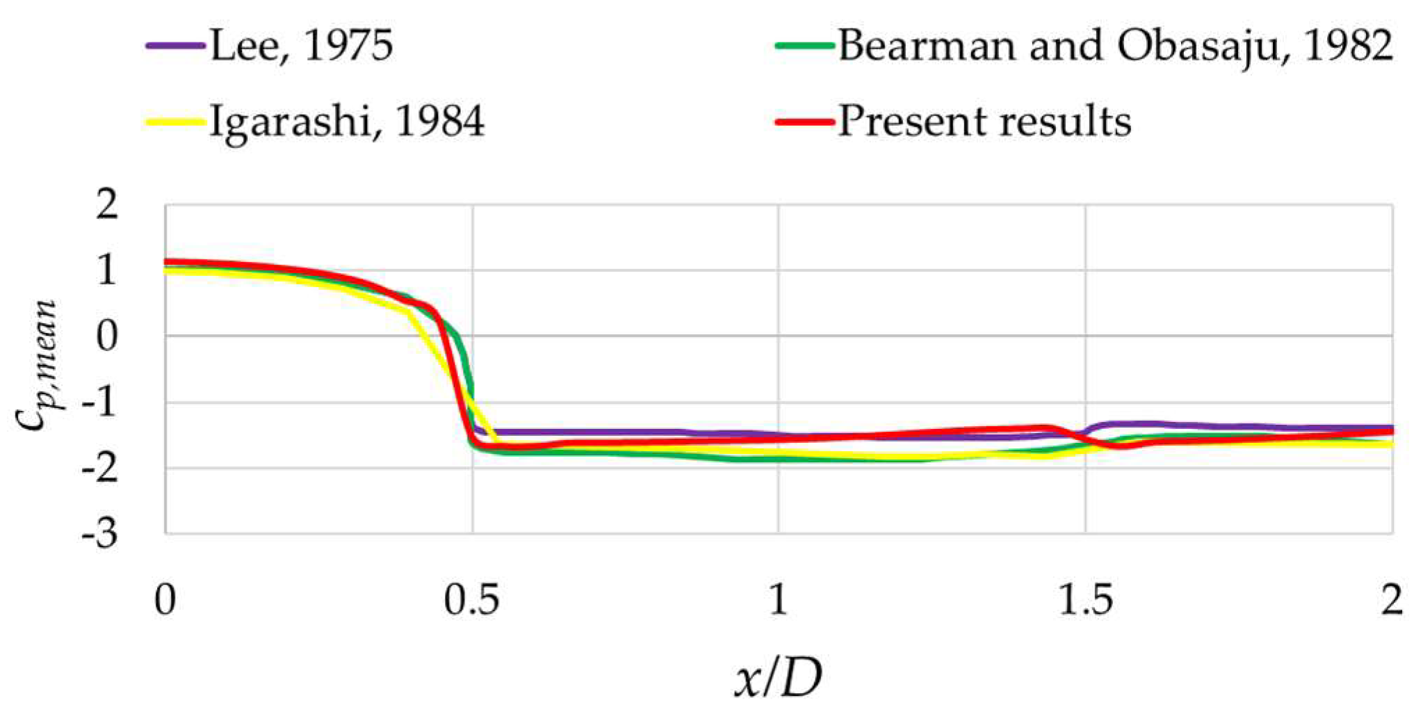
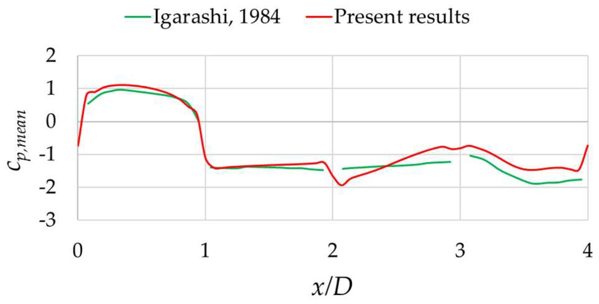
3.1. Numerical Results for Re = 2.2 × 10⁴ and Model Validation

Numerical results are presented in this section for Re = 2.2 × 10⁴ and various angles of incidence. Two different values, I = 0.05 and 0.2, of the turbulence intensity level at the inlet boundary were considered, with negligible differences on the final results; the ones with I = 0.05 are presented here. The results are compared with experimental data and with other numerical results from the literature (see Table 1) in order to validate the numerical modeling and analysis method used in this study.

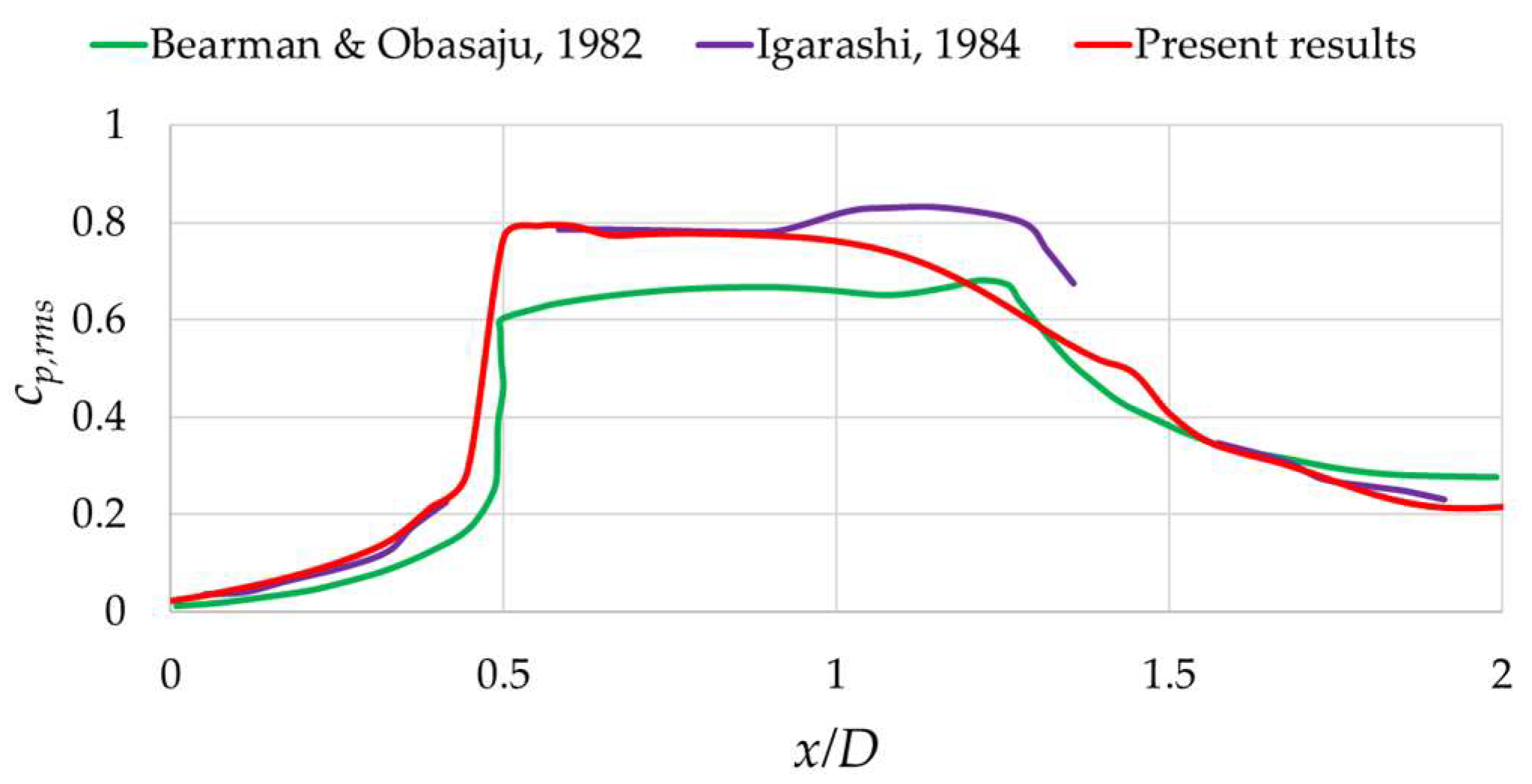
3.1.1. Zero-Degrees Angle of Incidence

In this section, numerical results for a zero-degrees angle of incidence and Re = 2.2 × 10⁴ are presented. As already mentioned, the frequency of vortex shedding in the wake of a square cross-section was used to define the dimensionless Strouhal number in Equation (2). Here, this frequency was computed, taking advantage of the fact that vortex shedding and lift force on the cross-section have the same oscillatory frequency. The lift coefficient time history is shown in Figure 4. Therefore, the shedding frequency was computed as the peak frequency of the fast Fourier transform of the lift coefficient time history (Figure 5). It is shown (Figure 5) that the time dependence of the lift coefficient is dominated by the main shedding vortex frequency in the wake of the cylinder, while the harmonic and sub-harmonic contributions are negligible.
In Figure 6, the instantaneous vorticity field around the square cross-section at the characteristic time instants A, B, and C of the lift coefficient time history, denoted in Figure 4, are illustrated for one period of vortex shedding. The vorticity contours are presented at these three characteristic instants for all examined cases throughout this study. It is observed that flow separation emanates at the upstream corners of the cross-section.
Based on the x coordinate along the perimeter of the square cross-section defined in Figure 7, the obtained mean pressure coefficient on the surface in Figure 8 and Figure 9 is compared with experimental and numerical results from the literature, respectively, for various Re values in the 104 to 105 range, exhibiting very good agreement. It is noted here that the comparison to flow results at Re of the same order but not of identical value (2.2 × 10⁴) is valid because, for this particular geometry, flow separation and turbulence development are strongly dictated by the sharp corners of the cross-section and weakly dictated by viscous effects, i.e., Re. Due to symmetry, the distribution is only presented along the upper half of the cross-section.
In Figure 10, corresponding results for the cp,rms distribution are illustrated. The maximum cp,rms is observed at the lateral sides of the cross-section due to the alternate shedding of vortices, while at the windward side, cp,rms has values gradually varying from 0 to 0.2, and at the leeward side from 0.4 to 0.3. As shown in both works [20,21], whose data are shown in Figure 10, the fluctuating pressure distribution is a very sensitive quantity, especially along the lateral and the leeward sides of the cross-section, and substantial differences are observed, even among experimental works; see, for example, Figure 5 in Bearman and Obasaju [20]. Therefore, the deviation between our results and the experimental ones are within the sensitivity range for this quantity.
Further comparisons of obtained results with experimental and numerical results from the literature are listed in Table 1 and Table 2, respectively. For the numerical results from the literature, the numerical method which was used is also provided. A good match was observed.

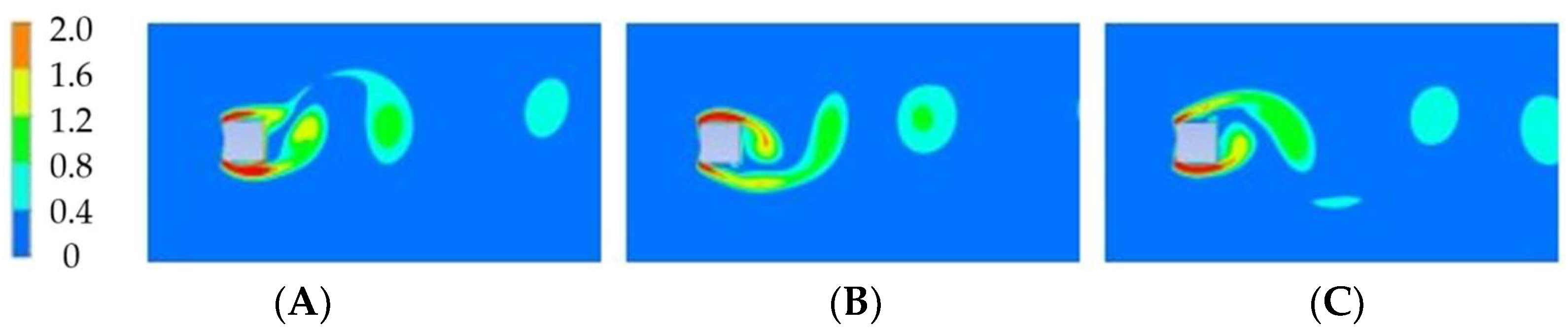
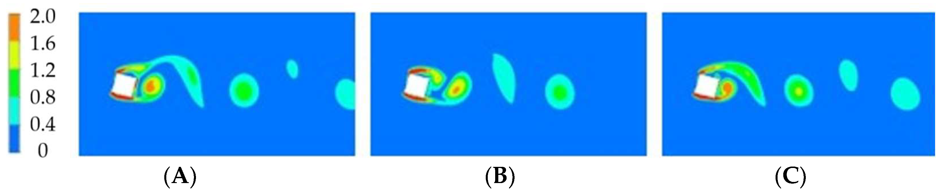
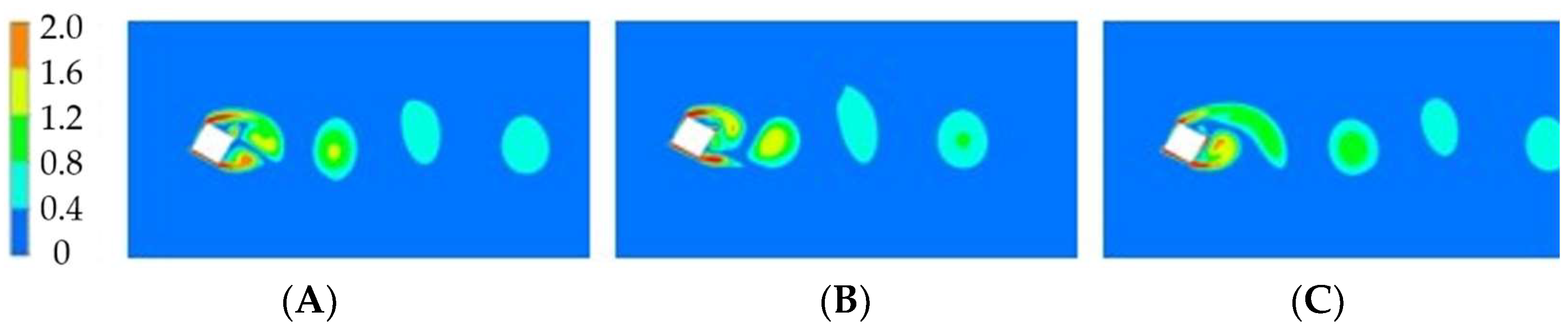
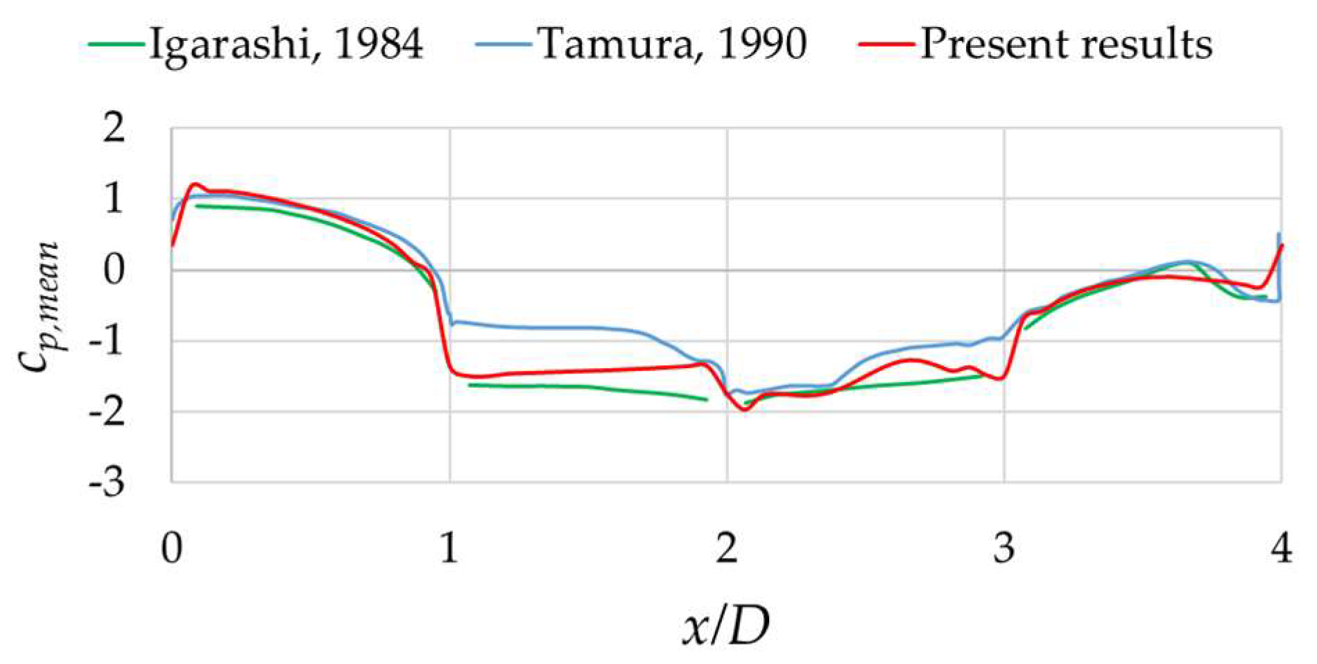
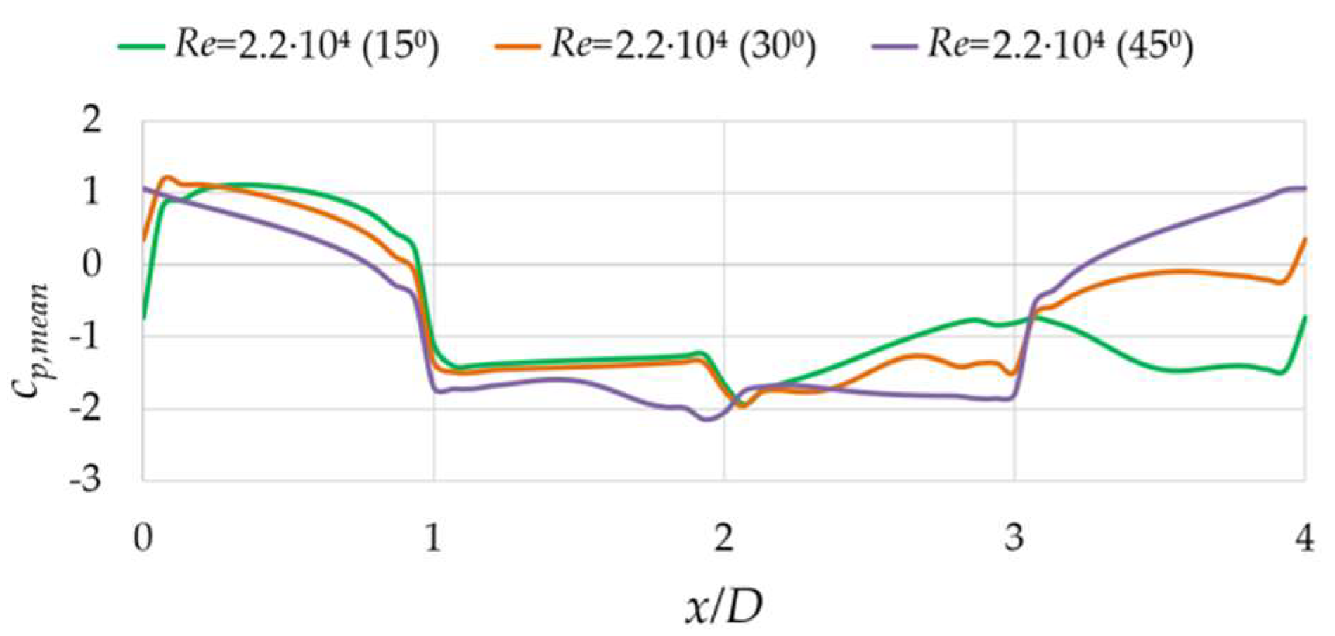
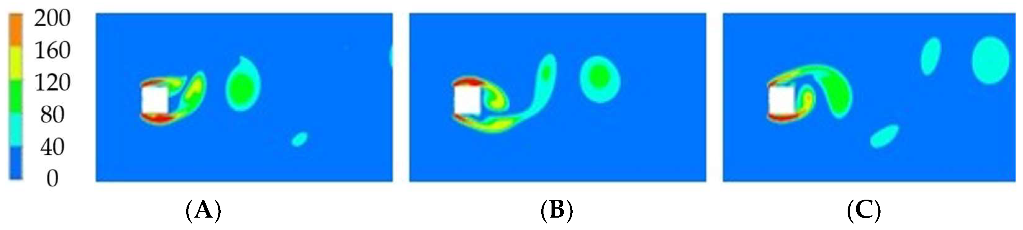
3.1.2. Nonzero Angles of Incidence

Next, a parametric study was conducted to obtain pressure coefficient distributions for various angle of incidence values, α, up to 45°. The vorticity fields at the three characteristic instants (A, B, and C) of the lift coefficient time history for α = 15°, 30°, and 45° are depicted in Figure 11, Figure 12 and Figure 13, respectively. Compared to the case of a zero-degrees angle of incidence, the flow separation at α = 15° and 30° may also emanate at the two upstream corners of the cross-section or even a downstream one, as α increases (Figure 11 and Figure 12). For the case of α = 45°, the flow separation emanates at the two symmetrical corners of the cross-section (Figure 13).
The mean pressure coefficient distributions for the various angles of incidence are presented along the perimeter of the square cross-section, as defined in Figure 14. The computed pressure coefficient distributions are compared with experimental [21] and numerical results [31,48] in Figure 15, Figure 16 and Figure 17, confirming that the k-ω (SST) turbulence model with the standard wall function approach is capable of effectively capturing the pressure coefficient distribution on a square cross-section for various angles of incidence.
The obtained results of the mean pressure coefficient distributions for various angles of incidence at Re = 2.2 × 10⁴ are compared in Figure 18. No significant differences are observed on the windward side (0–1), while larger values of cp,mean are observed at the sides 1–2 and 2–3, gradually increasing as the angle of incidence increases and reaches the maximum value for α = 45°.

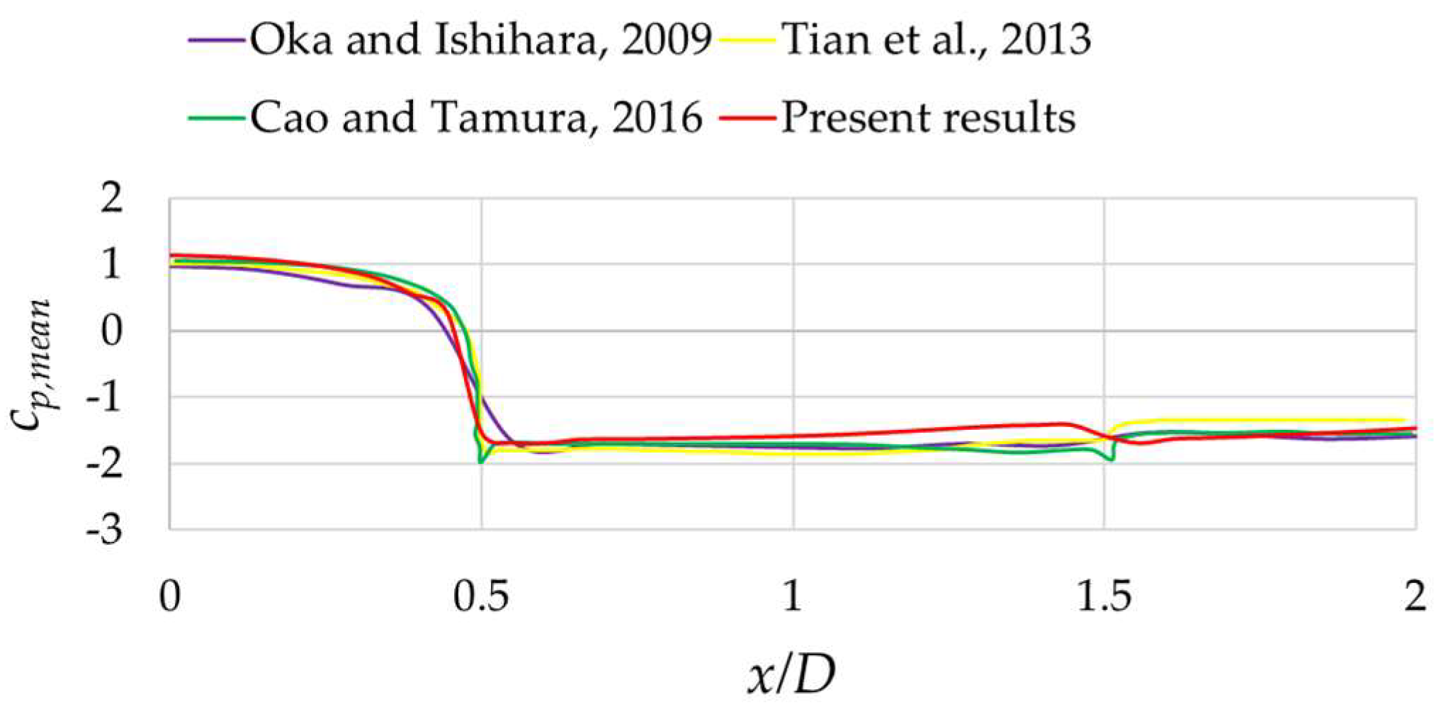
3.2. Numerical Results for High Reynolds Numbers

In this section, the airflow around the square cross-section at higher Re values is investigated, obtaining numerical results for Re = 2 × 10⁶ and Re = 107, and comparing them with the corresponding ones for Re = 2.2 × 10⁴. The high Re cases are investigated because in the wind flow around buildings, Re values larger than 5 × 10⁶ are developing. Thus, the resulting pressure coefficient distributions constitute an estimation of the wind actions to be considered for the structural design of buildings. For such higher Re values, not many results can be found in the literature, particularly for nonzero angles of incidence. Two different values of the turbulence intensity level at the inlet boundary, I = 0.05 and 0.2, are considered with negligible differences on the final results; the ones with I = 0.2 are presented here. According to EN1991-1-4 [37], the value I = 0.2 corresponds to a relatively high level of incident flow turbulence on tall buildings.

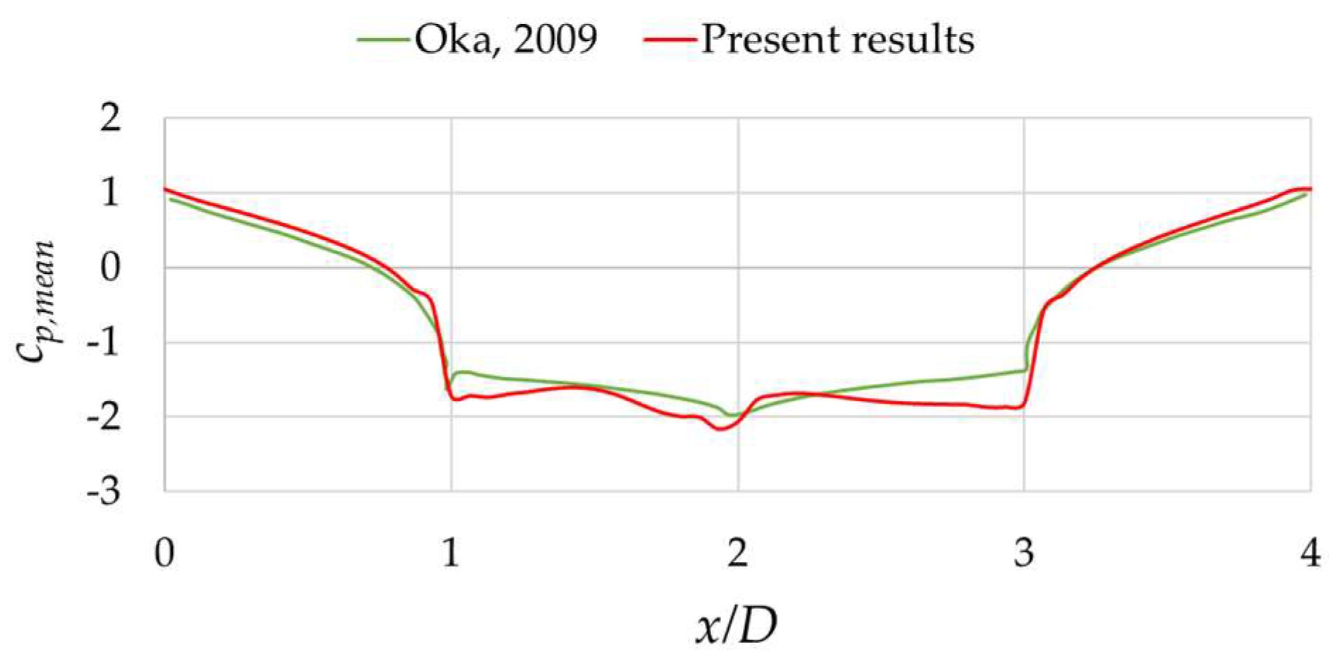
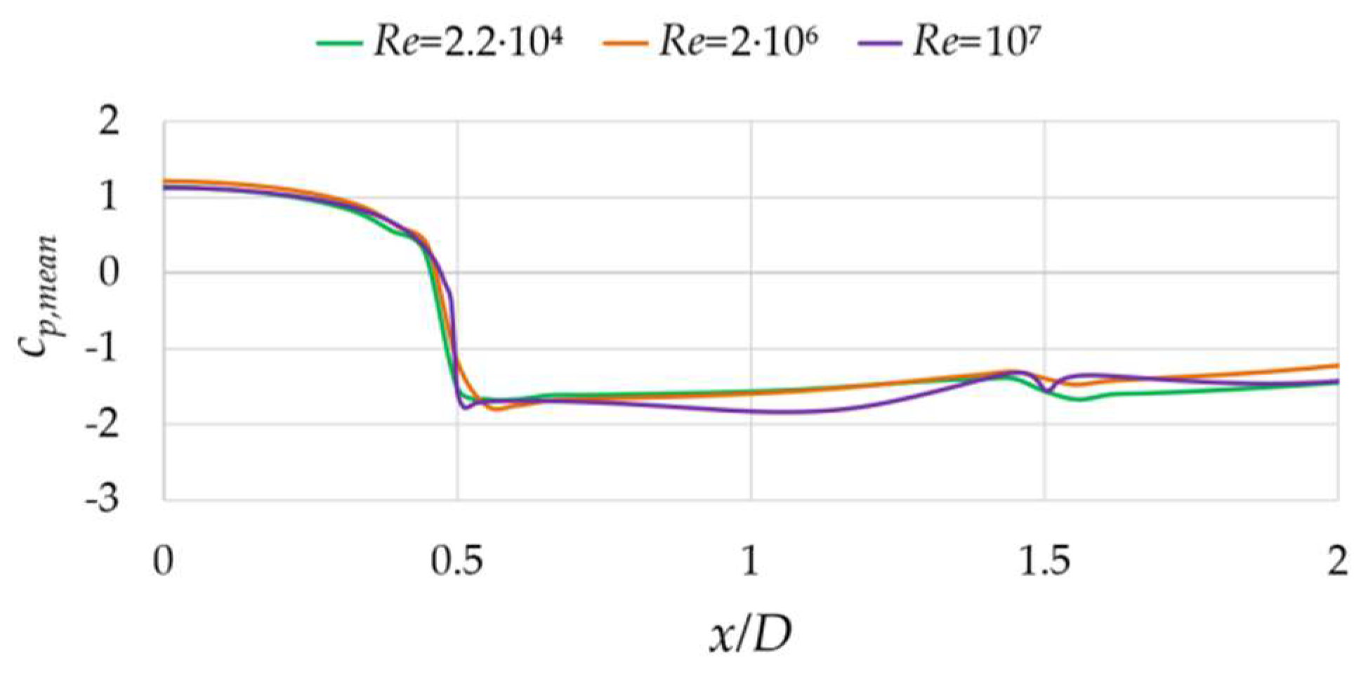
3.2.1. Zero-Degrees Angle of Incidence

For a zero-degrees angle of incidence, the results are also compared with the experimental data of Delany et al.’s study [17] and the numerical results of Sohankar’s study [30], based on the LES approach, along with provisions of EN1991-1-4 [37] and AS/NZS [38]. The presented pressure coefficient distribution from the EN1991-1-4 refers to buildings with AR = 5. For buildings with high AR values, the flow in the middle part is considered to approach 2D conditions [39,40].
The oscillating nature of the flow separation is present at the high Re cases as well, as highlighted in Figure 19 and Figure 20 where the instantaneous vorticity contours are shown for Re = 2 × 10⁶ and 107, respectively, for a zero-degrees angle of incidence. Alternate vortices at the downstream side of the square cross-section at the characteristic time instants of the lift coefficient time history are also observed in Figure 19 and Figure 20. The increase in the Re number is achieved by an increase of a factor of five in the incoming velocity magnitude. The resulting vorticity magnitude, both in the boundary layers and in the wake, also increased by a factor of about five.
For a zero-degrees angle of incidence, the dependence of the mean drag coefficient, the drag rms, the lift rms, and the St number in the range 5 × 10³ to 107 is presented in Table 3. The present results are compared with available results from the literature [17,30], exhibiting a satisfactory match.
As illustrated in Table 3, the cf,mean value increases slightly as the Reynolds number increases from 5 × 10³ to 107. The cf,rms value is almost unaffected by the Reynolds number, while cl,rms has a higher variation but without an obvious trend. The St number exhibits a significant reduction with increasing Re from low to medium values, but not from medium to higher ones.
A comparison of the distribution of mean and rms pressure coefficients for the examined Re numbers is presented in Figure 21 and Figure 22, respectively. It is concluded that an increase in the Re number does not significantly affect the max or min cp,mean and cp,rms values on the sides of the square cross-section for a zero-degrees angle of incidence.

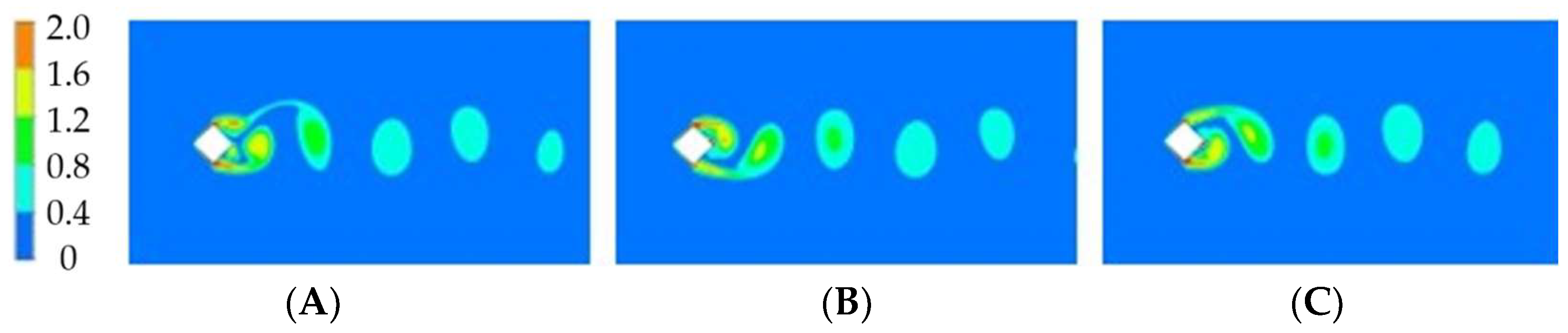
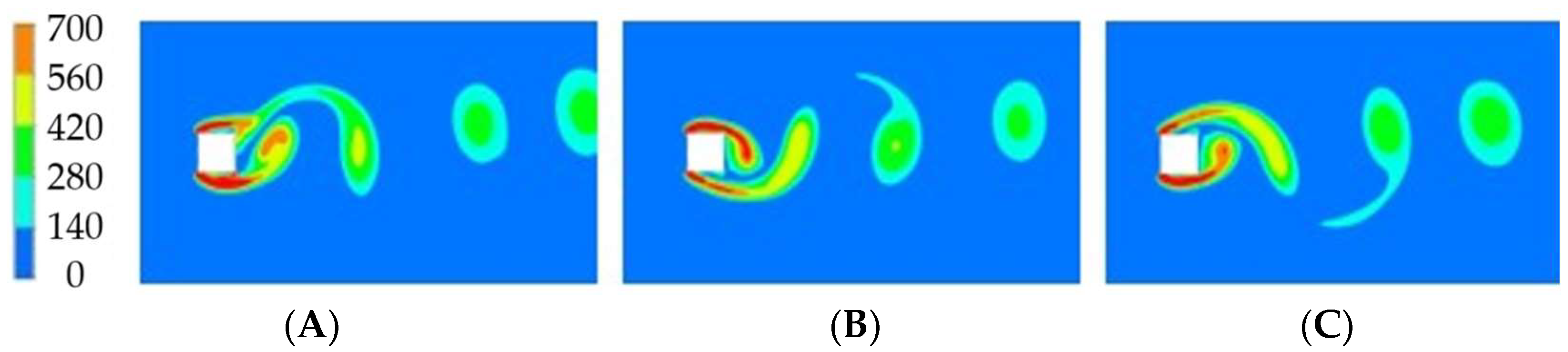
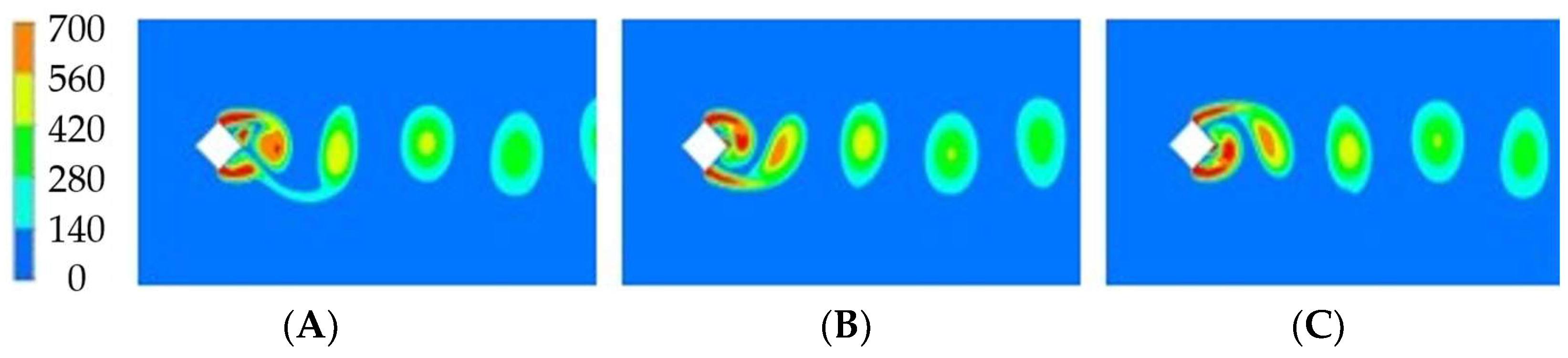
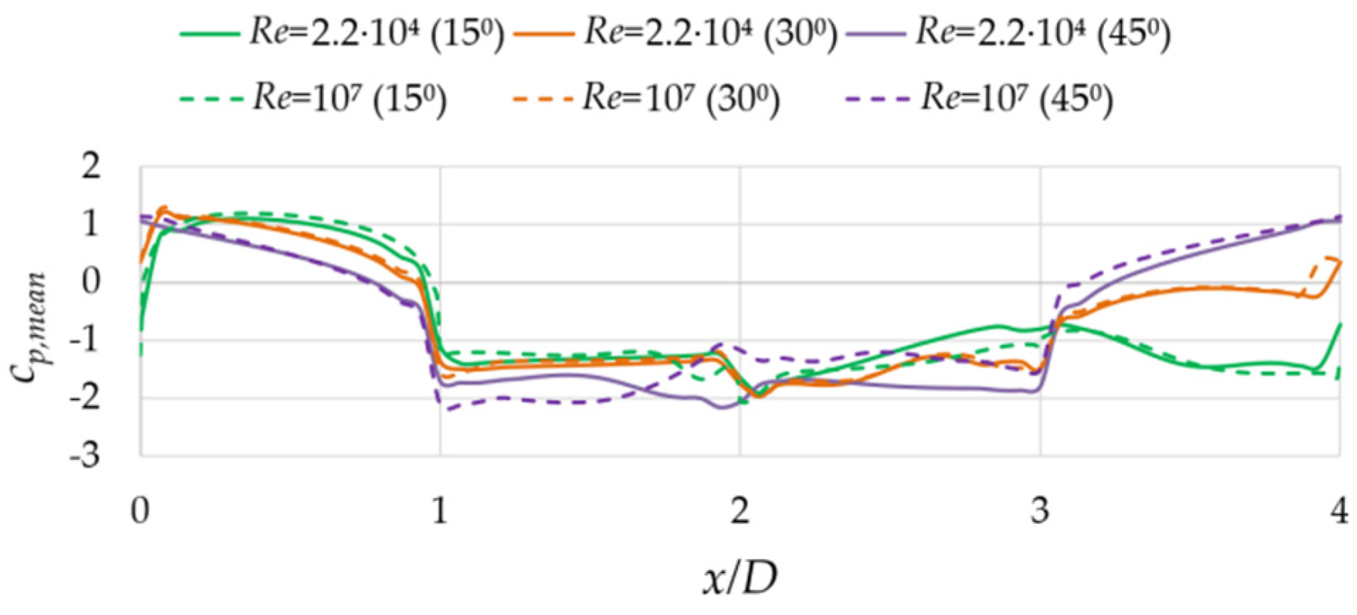
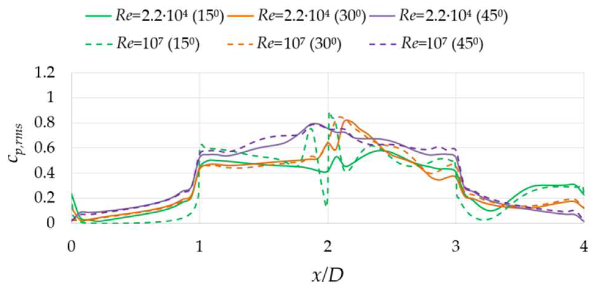
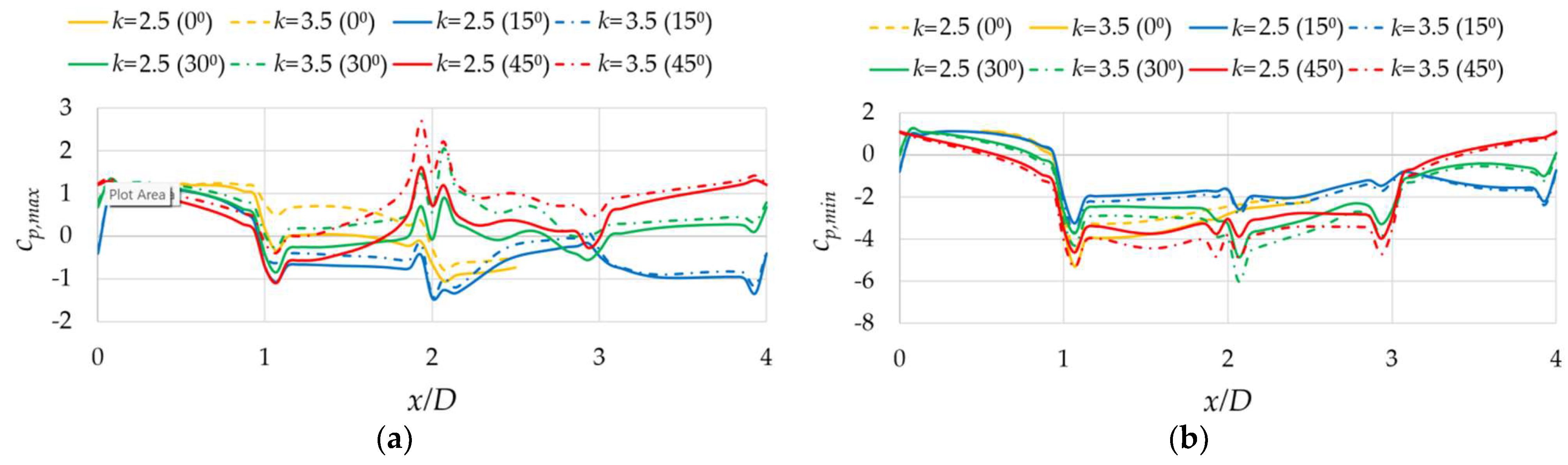
3.2.2. Nonzero Angles of Incidence

Similar analyses are carried out for Re = 107 and α = 15°, 30°, and 45°. The corresponding vorticity contours are shown in Figure 23, Figure 24 and Figure 25. Τhe development of the vortex shedding effect is demonstrated. While flow separation emanates at the two upstream corners of the square cross-section for a zero-degrees angle of incidence, for nonzero angles, it may emanate at a downstream corner as well. For the case of α = 45°, flow separation emanates at the two symmetrical corners. For α = 15° and 30°, the asymmetry of the wake is demonstrated in Figure 23 and Figure 24. Vortices are generated at the upper and lower sides of the square cross-section due to boundary layer separation (Figure 23, Figure 24 and Figure 25).
The mean pressure coefficient distribution results for Re = 107 are shown with dashed lines in Figure 26, while the corresponding results for Re = 2.2 × 10⁴ are presented with continuous lines. The cp,mean increases on sides 3–4 as the angle of incidence increases. On sides 1–2 and 2–3, differences between the two Re numbers in the ranges of 15% and 38%, respectively, are observed for α = 45°. In all other cases, the differences are smaller, i.e., around 5%.
The rms pressure coefficients for Re = 107 are shown with dashed lines in Figure 27, while the corresponding results for Re = 2.2 × 10⁴ are presented with continuous lines, exhibiting non-negligible differences. As the angle of incidence increases, the rms values on sides 1–2 and 2–3 increase by an average of 20%, while on sides 0–1 and 3–4, the effect is smaller.

4. Discussion

As already mentioned, the obtained results for 2D conditions are considered to be representative for the middle parts of buildings with a square cross-section and high AR (>>5) values, far from the roof and the ground, and at several angles of incidence. Typical Re values for such problems are larger than 106, for which limited experimental and numerical results are available in the literature. While the structural design against wind actions for buildings with AR ≤ 5 is based on the distribution of the pressure coefficient, cp, along the surfaces of the walls and roof, for AR > 5, the pertinent codes only propose values of the force (drag) coefficient, cf, per unit height of the building. Such values are sufficient for accounting for the wind effects on the main structural system of the building as a whole, but cannot predict the local effects of wind on the secondary structural system by supporting the building façade or cladding elements.
For this purpose, the highest local wind pressure values must be employed, which are estimated here through the use of the peak factor k. In other words, the maximum and minimum expected values of pressure coefficients are estimated, according to Equations (11) and (12), for peak factors equal to k = 2.5 and k = 3.5, to cover a range of k values proposed in the literature [45,46,47,48]. Corresponding results are presented in Figure 28 for a zero-degrees angle of incidence and in Figure 29a,b for all examined angles of incidence.
For a zero-degrees angle of incidence, the effect of the peak factor k on the max/min pressure coefficient values is larger at the sides of the bluff body and is less significant at the windward and leeward sides. As shown in Figure 29a, the highest maximum values are observed on sides 1–2 for α = 0° and α = 45°. On sides 3–4, the highest maximum values occurred for α = 45°. On the windward side, the maximum and minimum values of the pressure coefficient present small differences for all examined angles of incidences. The highest cp,min values occur on sides 1–2 and 2–3 for α = 30° and α = 45°, as presented in Figure 29b.

5. Conclusions

Τhe airflow over a square cylinder at high Reynolds numbers for various angles of incidence was investigated by employing URANS equations using the wall function approach. The simulations were performed using the k-ω (SST) turbulence model. This numerical approach was validated by comparing time-averaged and rms quantities of the aerodynamic coefficients for Re = 2.2 × 10⁴ with experimental and numerical results from the literature.
The numerical analyses were then extended to higher Re cases, representative of wind flow around tall buildings. The magnitude of the pressure coefficients was found to increase with increasing Re and increasing α. The computed values are significantly higher than the ones provided in EN1991-1-4 for structures with square cross-sections, which are limited to cases with α = 0° and buildings with AR ≤ 5. This study helps to address the gap in pressure coefficient data that can be used in the structural design of taller buildings with AR > 5, taking into account the effect of realistic high Re and nonzero α values, using URANS equations which may be employed in future work for other, more complex cross-sectional shapes, offering computational advantages. Due to the 2D nature of the presented computations, computed pressure coefficient distributions may be considered to be suitable for the design of secondary structural systems supporting the cladding in the middle parts of buildings with higher AR values where the flow resembles better 2D conditions.

Author Contributions

Conceptualization, A.C.K. and C.J.G.; methodology, A.C.K., A.A.D. and C.J.G.; software, A.C.K.; validation, A.C.K.; formal analysis, A.C.K.; investigation, A.C.K.; resources, A.C.K., A.A.D. and C.J.G.; data curation, A.C.K., A.A.D. and C.J.G.; writing—original draft preparation, A.C.K. and C.J.G.; writing—review and editing, A.C.K., A.A.D. and C.J.G.; visualization, A.C.K.; supervision, A.A.D. and C.J.G.; project administration, A.C.K. All authors have read and agreed to the published version of the manuscript.

Funding

This research received no external funding.

Data Availability Statement

Data are contained within the article.

Conflicts of Interest

The authors declare no conflicts of interest.

References

  1. Cook, N.; Mayne, J. A novel working approach to the assessment of wind loads for equivalent static design. J. Wind Eng. Ind. Aerodyn. 1979, 4, 149–164. [Google Scholar] [CrossRef]
  2. Cook, N.; Mayne, J. A refined working approach to the assessment of wind loads for equivalent static design. J. Wind Eng. Ind. Aerodyn. 1980, 6, 125–137. [Google Scholar] [CrossRef]
  3. Cook, N. Calibration of the quasi-static and peak-factor approaches to the assessment of wind loads against the method of Cook and Mayne. J. Wind Eng. Ind. Aerodyn. 1982, 10, 315–341. [Google Scholar] [CrossRef]
  4. Harris, R. An improved method for the prediction of extreme values of wind effects on simple buildings and structures. J. Wind Eng. Ind. Aerodyn. 1982, 9, 343–379. [Google Scholar] [CrossRef]
  5. Kwok, K. Cross-wind response of tall buildings. Eng. Struct. 1982, 4, 256–262. [Google Scholar] [CrossRef]
  6. Wacker, J.; Plate, E. Local peak wind pressure coefficients for cuboidal buildings and corresponding pressure gust factors. J. Wind Eng. Ind. Aerodyn. 1993, 50, 183–192. [Google Scholar] [CrossRef]
  7. Zhou, Y.; Kijewski, T.; Kareem, A. Aerodynamic Loads on Tall Buildings: Interactive Database. J. Struct. Eng. 2003, 129, 394–404. [Google Scholar] [CrossRef]
  8. Stathopoulos, T.; Baniotopoulos, C. Wind Effects on Buildings and Design of Wind-Sensitive Structures; Springer: Berlin/Heidelberg, Germany, 2007. [Google Scholar]
  9. Holmes, J.D. Wind Loading of Structures; Taylor & Francis: London, UK, 2007. [Google Scholar]
  10. Petrini, F.; Ciampoli, M. Performance-based wind design of tall buildings. Struct. Infrastruct. Eng. 2012, 8, 954–966. [Google Scholar] [CrossRef]
  11. Dagnew, A.; Bitsuamlak, G. Computational evaluation of wind loads on a standard tall building using LES. Wind Struct. 2014, 18, 567–598. [Google Scholar] [CrossRef]
  12. Rizzo, F.; D’Alessandro, V.; Montelpare, S.; Giammichele, L. Computational study of a bluff body aerodynamics: Impact of the laminar-to-turbulent transition modelling. Int. J. Mech. Sci. 2020, 178, 105620. [Google Scholar] [CrossRef]
  13. Rizzo, F.; Huang, M. Peak value estimation for wind-induced lateral accelerations in a high-rise building. Struct. Infrastruct. Eng. 2021, 18, 1317–1333. [Google Scholar] [CrossRef]
  14. Rizzo, F. Sensitivity Investigation on the Pressure Coefficients Non-Dimensionalization. Infrastructures 2021, 6, 53. [Google Scholar] [CrossRef]
  15. Petrini, F.; Li, H.; Bontempi, F. Basis of design and numerical modeling of offshore wind turbines. Struct. Eng. Mech. 2010, 36, 599. [Google Scholar] [CrossRef]
  16. Zou, Q.; Li, Z.; Wu, H.; Kuang, R.; Hui, Y. Wind pressure distribution on trough concentrator and fluctuating wind pressure characteristics. Sol. Energy 2015, 120, 464–478. [Google Scholar] [CrossRef]
  17. Delany, N.K.; Sorensen, N.E. Low-Speed Drag of Cylinders of Various Shape; National Advisory Committee for Aeronautics: Washington, DC, USA, 1953. [Google Scholar]
  18. Vickery, B.J. Fluctuating lift and drag on a long cylinder of square cross-section in a smooth and in a turbulent stream. J. Fluid Mech. 1966, 25, 481–494. [Google Scholar] [CrossRef]
  19. Lee, B.E. The effect of turbulence on the surface pressure field of a square prism. J. Fluid Mech. 1975, 69, 263–282. [Google Scholar] [CrossRef]
  20. Bearman, P.W.; Obasaju, E.D. An experimental study of pressure fluctuations on fixed and oscillating square-section cylinders. J. Fluid Mech. 1982, 119, 297–321. [Google Scholar] [CrossRef]
  21. Igarashi, T. Characteristics of the Flow around a Square Prism. Bull. JSME 1984, 27, 1858–1865. [Google Scholar] [CrossRef]
  22. Knisely, C.W. Strouhal numbers of rectangular cylinders at incidence: A review and new data. J. Fluids Struct. 1990, 4, 371–393. [Google Scholar] [CrossRef]
  23. Norberg, C. Flow around rectangular cylinders: Pressure forces and wake frequencies. J. Wind Eng. Ind. Aerodyn. 1993, 49, 187–196. [Google Scholar] [CrossRef]
  24. Luo, S.; Yazdani, M.; Chew, Y.; Lee, T. Effects of incidence and afterbody shape on flow past bluff cylinders. J. Wind Eng. Ind. Aerodyn. 1994, 53, 375–399. [Google Scholar] [CrossRef]
  25. Lyn, D.A.; Einav, S.; Rodi, W.; Park, J.-H. A laser-Doppler velocimetry study of ensemble-averaged characteristics of the turbulent near wake of a square cylinder. J. Fluid Mech. 1995, 304, 285–319. [Google Scholar] [CrossRef]
  26. Tamura, T.; Miyagi, T. The effect of turbulence on aerodynamic forces on a square cylinder with various corner shapes. J. Wind Eng. Ind. Aerodyn. 1999, 83, 135–145. [Google Scholar] [CrossRef]
  27. van Oudheusden, B.; Scarano, F.; van Hinsberg, N.; Roosenboom, E. Quantitative visualization of the flow around a square-section cylinder at incidence. J. Wind Eng. Ind. Aerodyn. 2008, 96, 913–922. [Google Scholar] [CrossRef]
  28. Carassale, L.; Freda, A.; Marrè-Brunenghi, M. Experimental investigation on the aerodynamic behavior of square cylinders with rounded corners. J. Fluids Struct. 2014, 44, 195–204. [Google Scholar] [CrossRef]
  29. van Hinsberg, N.P.; Schewe, G.; Jacobs, M. Experiments on the aerodynamic behaviour of square cylinders with rounded corners at Reynolds numbers up to 12 million. J. Fluids Struct. 2017, 74, 214–233. [Google Scholar] [CrossRef]
  30. Sohankar, A. Flow over a bluff body from moderate to high Reynolds numbers using large eddy simulation. Comput. Fluids 2006, 35, 1154–1168. [Google Scholar] [CrossRef]
  31. Oka, S.; Ishihara, T. Numerical study of aerodynamic characteristics of a square prism in a uniform flow. J. Wind Eng. Ind. Aerodyn. 2009, 97, 548–559. [Google Scholar] [CrossRef]
  32. Ying, X.; Zhang, Z. Prediction of Unsteady Flow around a Square Cylinder Using RANS. Appl. Mech. Mater. 2011, 52–54, 1165–1170. [Google Scholar]
  33. Tian, X.; Ong, M.C.; Yang, J.; Myrhaug, D. Unsteady RANS simulations of flow around rectangular cylinders with different aspect ratios. Ocean Eng. 2013, 58, 208–216. [Google Scholar] [CrossRef]
  34. Cao, Y.; Tamura, T. Large-eddy simulations of flow past a square cylinder using structured and unstructured grids. Comput. Fluids 2016, 137, 36–54. [Google Scholar] [CrossRef]
  35. Zhang, L.Z. Numerical Simulation of Flows past a Circular and a Square Cylinder at High Reynolds Number, and a Curved Plate in Transitional Flow. Master’s Thesis, Washington University, St. Louis, MO, USA, 2017. [Google Scholar]
  36. Dai, S.S.; Younis, B.A.; Zhang, H.Y. Prediction of Turbulent Flow Around a Square Cylinder With Rounded Corners. J. Offshore Mech. Arct. Eng. 2017, 139, 031804. [Google Scholar] [CrossRef]
  37. EN1991-1-4:2005/AC:2010 (E); Eurocode 1: Actions on Structures—Part 1–4: General Actions—Wind Actions. European Standard (Eurocode); European Committee for Standardization (CEN): Bruxelles, Belgium, 2010.
  38. AS/NZS, 1170,2:2002; Structural Design Actions, Part 2: Wind Actions. Standards Australia: Sydney, Australia; Standards New Zealand: Wellington, New Zealand, 2002.
  39. Okamoto, S.; Uemura, N. Effect of rounding side-corners on aerodynamic forces and turbulent wake of a cube placed on a ground plane. Exp. Fluids 1991, 11, 58–64. [Google Scholar] [CrossRef]
  40. McClean, J.; Sumner, D. An Experimental Investigation of Aspect Ratio and Incidence Angle Effects for the Flow Around Surface-Mounted Finite-Height Square Prisms. J. Fluids Eng. 2014, 136, 081206. [Google Scholar] [CrossRef]
  41. Fluent, ANSYS FLUENT 19.2 Theory Guide; Ansys Inc.: Canonsburg, PA, USA.
  42. Menter, F.R. Two-equation eddy-viscosity turbulence models for engineering applications. AIAA J. 1994, 32, 1598–1605. [Google Scholar] [CrossRef]
  43. Menter, F.R. Zonal two equation kw turbulence models for aerodynamic flows. In Proceedings of the 23rd Fluid Dynamics, Plasmadynamics, and Lasers Conference, Orlando, FL, USA, 6–9 July 1993. [Google Scholar]
  44. Argyropoulos, C.D.; Markatos, N.C. Recent advances on the numerical modelling of turbulent flows. Appl. Math. Model. 2015, 39, 693–732. [Google Scholar] [CrossRef]
  45. Elshaer, A.; Aboshosha, H.; Bitsuamlak, G.; El Damatty, A.; Dagnew, A. LES evaluation of wind-induced responses for an isolated and a surrounded tall building. Eng. Struct. 2016, 115, 179–195. [Google Scholar] [CrossRef]
  46. Elshaer, A.; Bitsuamlak, G.; El Damatty, A. Enhancing wind performance of tall buildings using corner aerodynamic optimization. Eng. Struct. 2017, 136, 133–148. [Google Scholar] [CrossRef]
  47. Sun, X.; Liu, H.; Su, N.; Wu, Y. Investigation on wind tunnel tests of the Kilometer skyscraper. Eng. Struct. 2017, 148, 340–356. [Google Scholar] [CrossRef]
  48. Tamura, T.; Ohta, I.; Kuwahara, K. On the reliability of two-dimensional simulation for unsteady flows around a cylinder-type structure. J. Wind Eng. Ind. Aerodyn. 1990, 35, 275–298. [Google Scholar] [CrossRef]
Figure 1. Sketch and main dimensions of a typical building with a square plan view.
Buildings 14 00561 g001
Figure 2. (a) Computational fluid domain; (b) details of the bluff body and angles of incidence (α).
Buildings 14 00561 g002
Figure 3. (a) Mesh of the computational domain; (b) details of the mesh around the square cross-section.
Buildings 14 00561 g003
Figure 4. Lift coefficient (cl) time history for a zero-degrees angle of incidence (Re = 2.2 × 10⁴).
Buildings 14 00561 g004
Figure 5. Fast Fourier transform of the lift coefficient time history for a zero-degrees angle of incidence (Re = 2.2 × 10⁴).
Buildings 14 00561 g005
Figure 6. Vorticity magnitude (s−1) for a zero-degrees angle of incidence (Re = 2.2 × 10⁴) at the characteristic time instants (AC) (from left to right) shown in Figure 4.
Buildings 14 00561 g006
Figure 7. Characteristic points of the pressure coefficient distribution along the perimeter of the square cross-section for a zero-degrees angle of incidence.
Buildings 14 00561 g007
Figure 8. Comparison of computed cp,mean values for a zero-degrees angle of incidence and Re = 2.2 × 10⁴ with experimental results for Re values in the 104 to 105 range [19,20,21].
Buildings 14 00561 g008
Figure 9. Comparison of computed cp,mean values for a zero-degree angle of incidence and Re = 2.2 × 10⁴ with numerical results for Re values in the 104 to 105 range [31,33,34].
Buildings 14 00561 g009
Figure 10. Comparison of computed cp,rms values with experimental results for a zero-degrees angle of incidence (Re = 2.2 × 10⁴) [20,21].
Buildings 14 00561 g010
Figure 11. Vorticity magnitude (s−1) for Re = 2.2 × 10⁴ and α = 15° at the characteristic time instants (AC) (from left to right) shown in Figure 4.
Buildings 14 00561 g011
Figure 12. Vorticity magnitude (s−1) for Re = 2.2 × 10⁴ and α = 30° at the characteristic time instants (AC) (from left to right) shown in Figure 4.
Buildings 14 00561 g012
Figure 13. Vorticity magnitude (s−1) for Re = 2.2 × 10⁴ and α = 45° at the characteristic time instants (AC) (from left to right) shown in Figure 4.
Buildings 14 00561 g013
Figure 14. Characteristic points of the pressure coefficient distribution along the perimeter of the square cross-section at a nonzero angle of incidence α.
Buildings 14 00561 g014
Figure 15. Comparison of computed cp,mean values with experimental results at Re = 2.2 × 10⁴ for α = 15° [21].
Buildings 14 00561 g015
Figure 16. Comparison of computed cp,mean values with experimental and numerical results at Re = 2.2 × 10⁴ for α = 30° [21,48].
Buildings 14 00561 g016
Figure 17. Comparison of computed cp,mean values with numerical results at Re = 2.2 × 10⁴ for α = 45° [31].
Buildings 14 00561 g017
Figure 18. Mean pressure (cp,mean) coefficient distribution at Re = 2.2 × 10⁴ for various angles of incidence.
Buildings 14 00561 g018
Figure 19. Vorticity magnitude (s−1) for a zero-degrees angle of incidence (Re = 2 × 10⁶) at the characteristic time instants (AC) (from left to right) shown in Figure 4.
Buildings 14 00561 g019
Figure 20. Vorticity magnitude (s−1) contours for a zero-degrees angle of incidence (Re = 107) at the characteristic time instants (AC) (from left to right) shown in Figure 4.
Buildings 14 00561 g020
Figure 21. Mean pressure coefficient distribution for a zero-degrees angle of incidence.
Buildings 14 00561 g021
Figure 22. Rms pressure coefficient distribution for a zero-degrees angle of incidence.
Buildings 14 00561 g022
Figure 23. Vorticity magnitude (s−1) contours for Re = 107 and α = 15° at the characteristic time instants (AC) (from left to right) shown in Figure 4.
Buildings 14 00561 g023
Figure 24. Vorticity magnitude (s−1) contours for Re = 107 and α = 30° at the characteristic time instants (AC) (from left to right) shown in Figure 4.
Buildings 14 00561 g024
Figure 25. Vorticity magnitude (s−1) contours for Re = 107 and α = 45° at the characteristic time instants (AC) (from left to right) shown in Figure 4.
Buildings 14 00561 g025
Figure 26. Mean pressure coefficient distribution for various angles of incidence.
Buildings 14 00561 g026
Figure 27. Fluctuating pressure distribution for various angles of incidence at Re = 107.
Buildings 14 00561 g027
Figure 28. Maximum and minimum pressure coefficient values for a zero-degrees angle of incidence.
Buildings 14 00561 g028
Figure 29. (a) Maximum and (b) minimum pressure coefficient values for all examined angles of incidence.
Buildings 14 00561 g029
Table 1. Comparison of aerodynamic coefficients with experimental results for a zero-degrees angle of incidence.
AuthorRe ( ×104)cf,meancf,rmscl,rmsSt
Vickery [18]102.050.171.300.12
Lee [19]17.62.040.221.190.122
Bearman and Obasaju [20]2.22.10-1.201.13
Norberg [23]1.32.11--0.131
Luo et al. [24]3.42.210.181.210.13
Lyn et al. [25]2.142.10--0.132
Tamura and Miyagi [26]32.10-1.050.13
Van Oudheusden et al. [27]22.19---
Carassale et al. [28]372.06-1.020.125
Our study2.22.090.1581.170.134
Table 2. Comparison of aerodynamic coefficients with numerical results for a zero-degrees angle of incidence.
AuthorMethodRe (×104)cf,meancf,rmscL,rmsSt
Sohankar [30]LESs2.22.250.2001.500.130
Oka and Ishihara [31]LESs12.060.1401.260.125
Xu and Zhang [32]URANS2.142.09-1.390.121
Tian et al. [33]URANS2.142.06-1.490.138
Cao and Tamura [34]LESs2.22.210.2051.260.132
Zhang [35]URANS2.22.20---
Dai et al. [36]URANS22.000.2041.130.130
Our studyURANS2.22.090.1581.170.134
Table 3. Aerodynamic coefficients with respect to Re.
ReVariableOur StudyDelany et al. [17]Sohankar [30]EN1991-1-4 [37]
5 × 10³–5 × 10⁴cf,mean2.091.92.242.1
cf,rms0.16-0.2-
cl,rms1.17-1.45-
St0.134-0.1230.12
3 × 10⁵–3 × 10⁶cf,mean2.281.952.292.1
cf,rms0.18-0.18-
cl,rms1.61-1.51-
St0.1-0.1280.12
4 × 10⁶–107cf,mean2.35-2.242.1
cf,rms0.15-0.2-
cl,rms1.37-1.58-
St0.1-0.1240.12
Disclaimer/Publisher’s Note: The statements, opinions and data contained in all publications are solely those of the individual author(s) and contributor(s) and not of MDPI and/or the editor(s). MDPI and/or the editor(s) disclaim responsibility for any injury to people or property resulting from any ideas, methods, instructions or products referred to in the content.

