
A New Method for Evaluating the Stability of Retaining Walls

Abstract
1. Introduction
2. Coulomb Retaining Walls
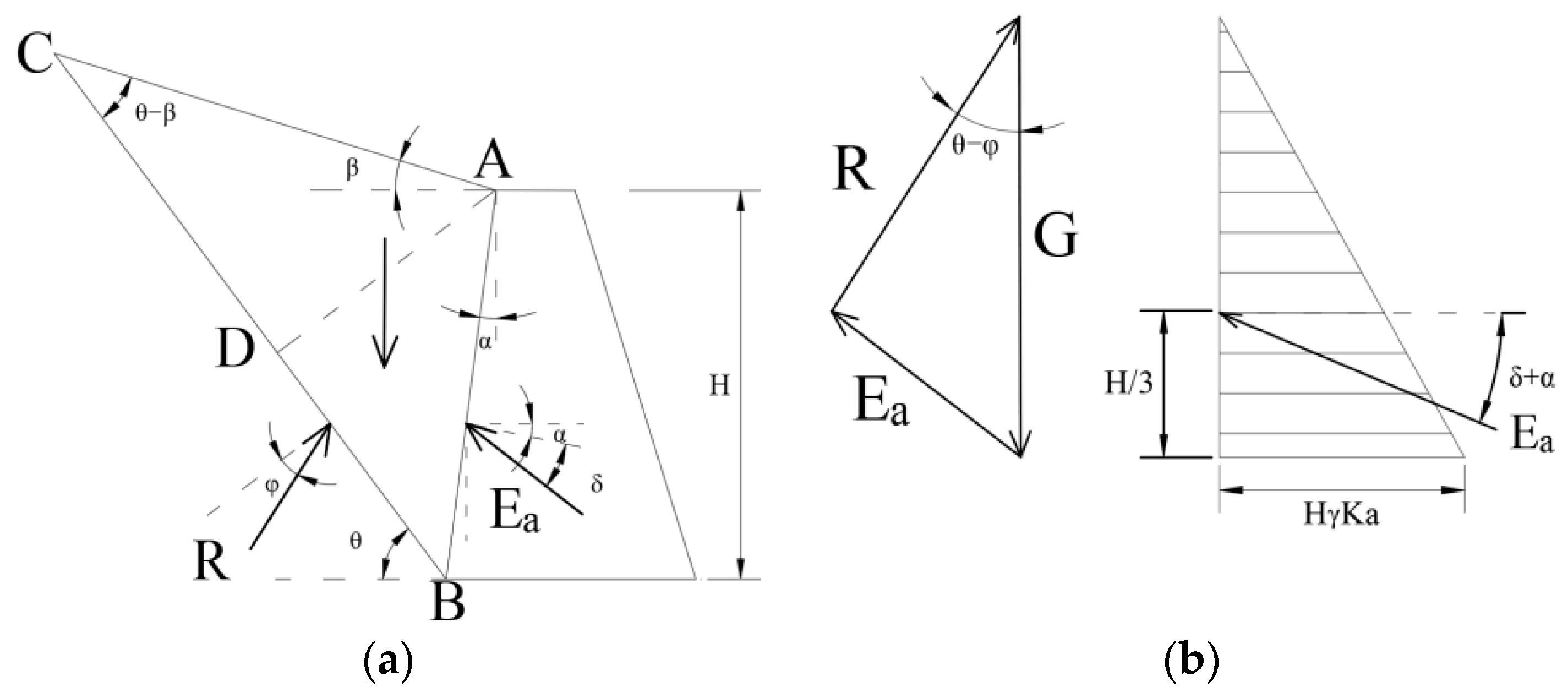
2.1. Active Earth Pressure
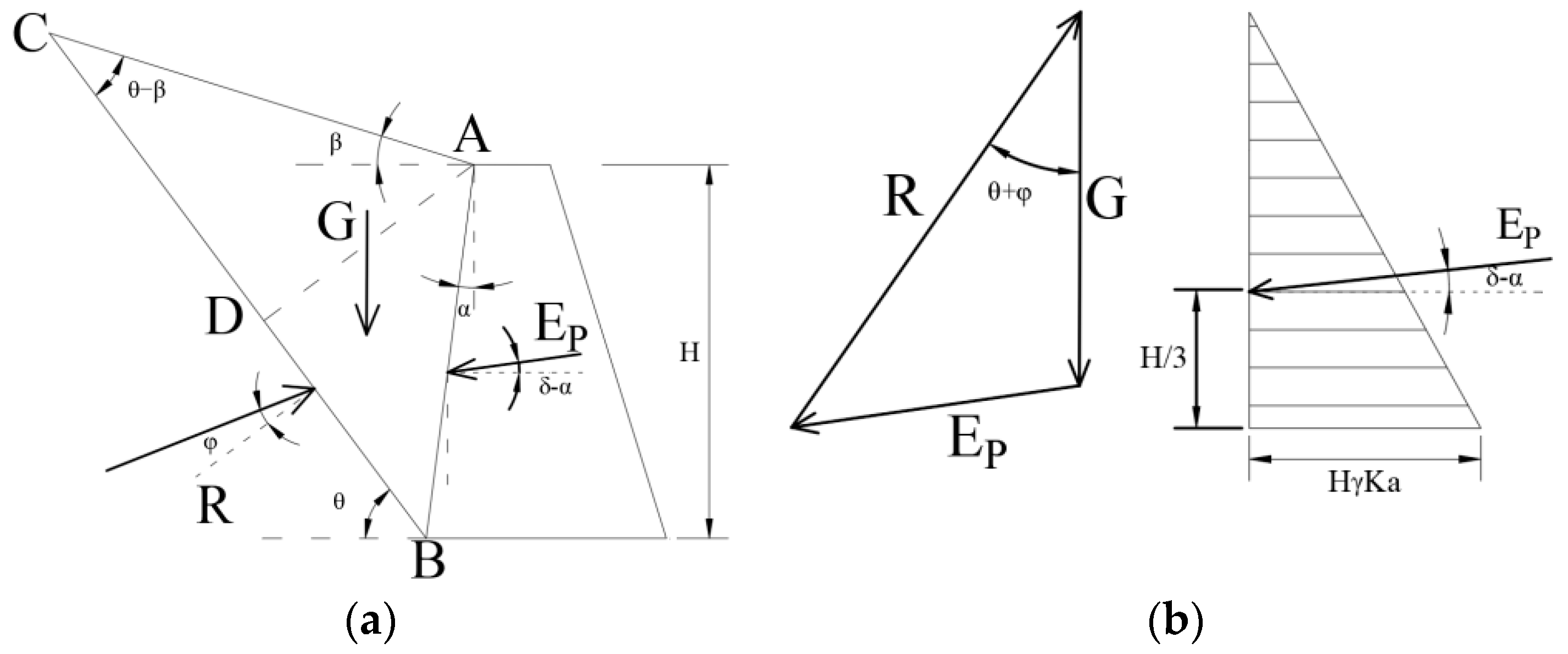
2.2. Passive Earth Pressure
2.3. Scientific Problems of Retaining Walls
3. Numerical Theoretical Solution of the Backfill Soil Wedge and Retaining Wall
3.1. Assumptions of the Soil Wedge and Retaining Wall
3.2. Boundary Conditions
3.3. Solution Steps
- (1)
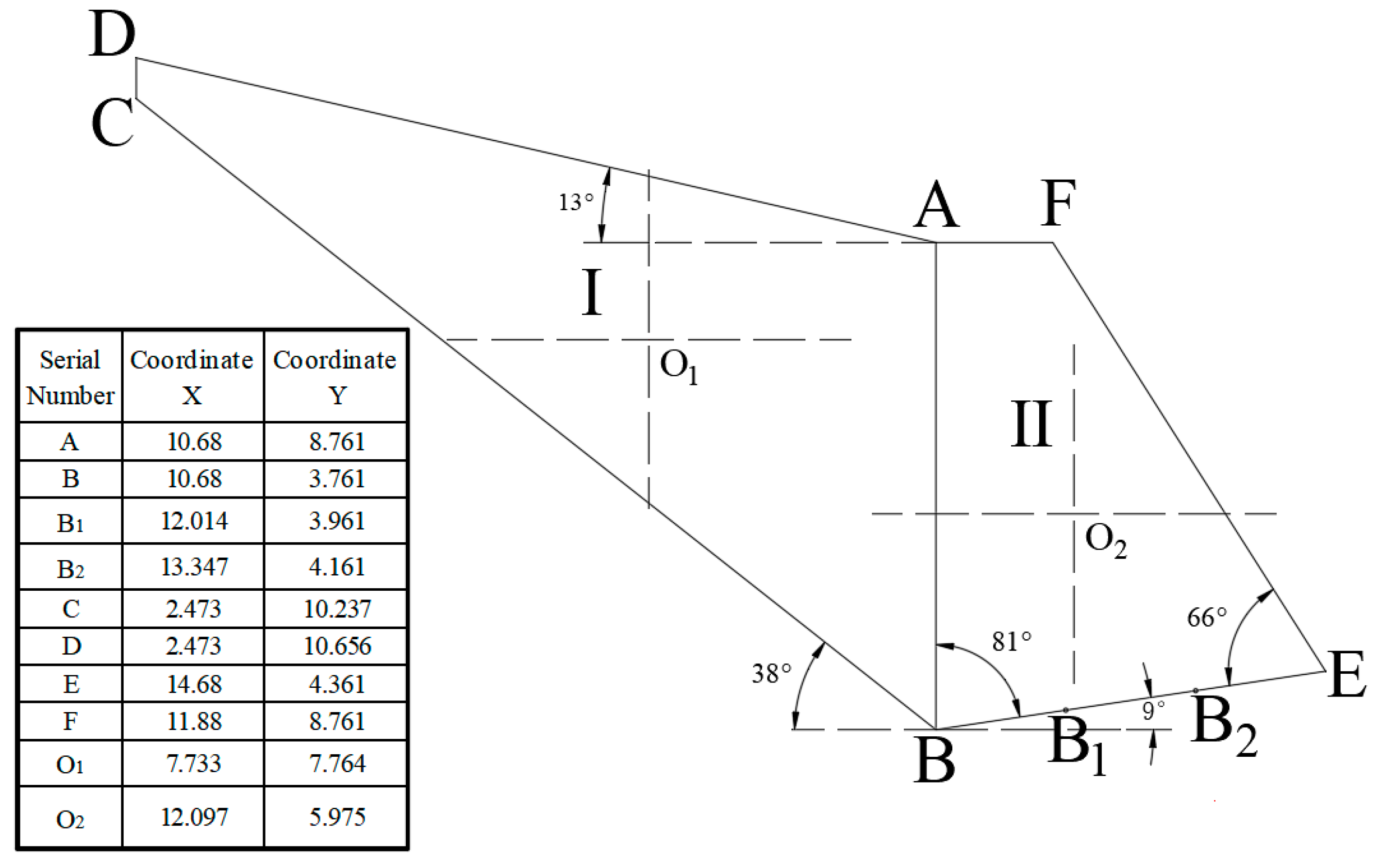
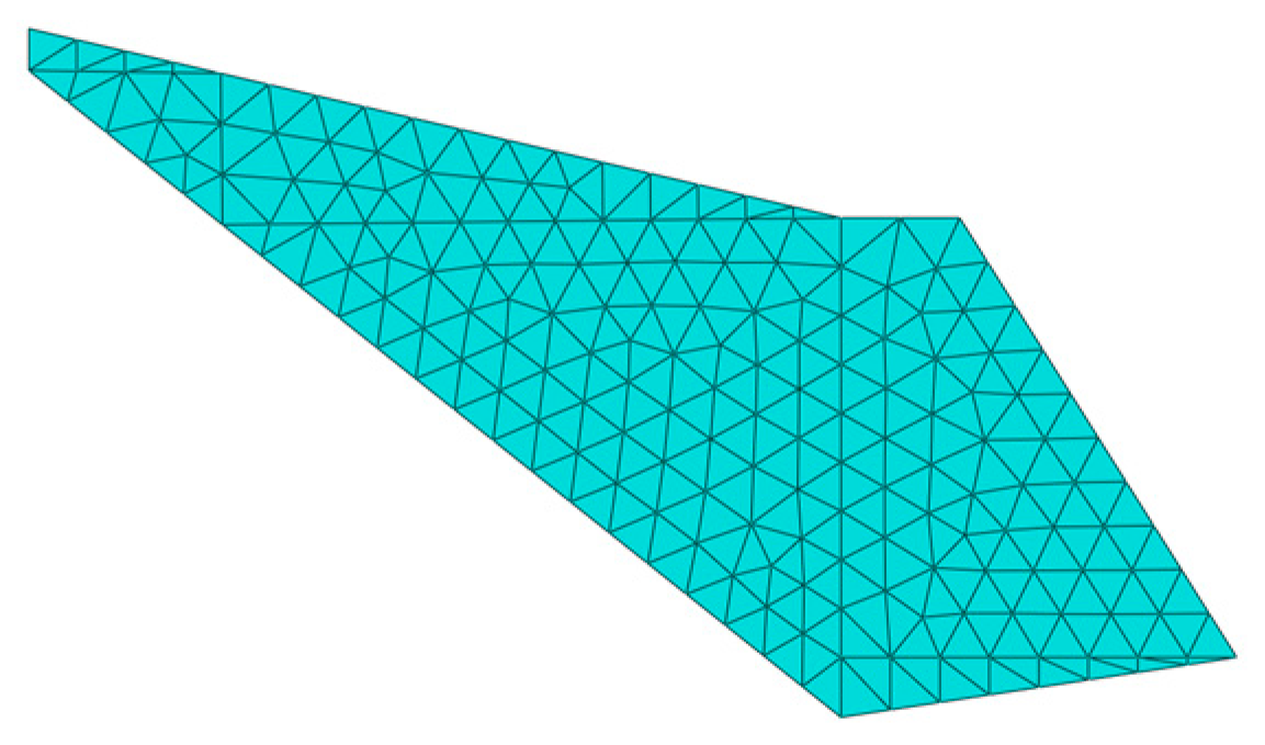
- Based on the cross-sectional view of the garbage transfer station in Lvcongpo Town, Badong County (see Section 4.2.1 below), a calculation model for the soil wedge and retaining wall is established, as shown in Figure 3. The model consists of two quadrilateral elements. Under a given plane coordinate system, the geometric characteristic equations related to each edge are expressed via .
- (2)
- The specific gravities of the soil wedge and retaining wall are constant. The expressions of the stress equations are selected, and the corresponding constant coefficients when the soil wedge and retaining wall satisfy the stress differential equilibrium equations, stress boundary conditions, and compatibility equations are calculated. The stress expressions are as follows:where are constant coefficients where i takes a value of zero and integers; denote the stresses in the X and Y directions and the shear stress, respectively; and represents the specific gravity in the Y direction. In the process of theoretical solution, the more high-order the stress expression is fitted and the more constant coefficients there are, the closer the obtained stress is to the actual situation. On the basis of previous studies, this study fits the stress expression in the form of a 5th power and obtains 33 unknown constant coefficients.
- (3)
- Taking the Y-axis as the perpendicular axis, the following equilibrium equations are satisfied under gravity conditions:
- (4)
- Making the corresponding coefficients zero is a necessary condition for the stress balance equation. Substituting the stress expression (20)–(22) into Equation (23) yields the following relationship:
4. Case Study
4.1. Division of Computation Units and Equations
4.2. Case Introduction
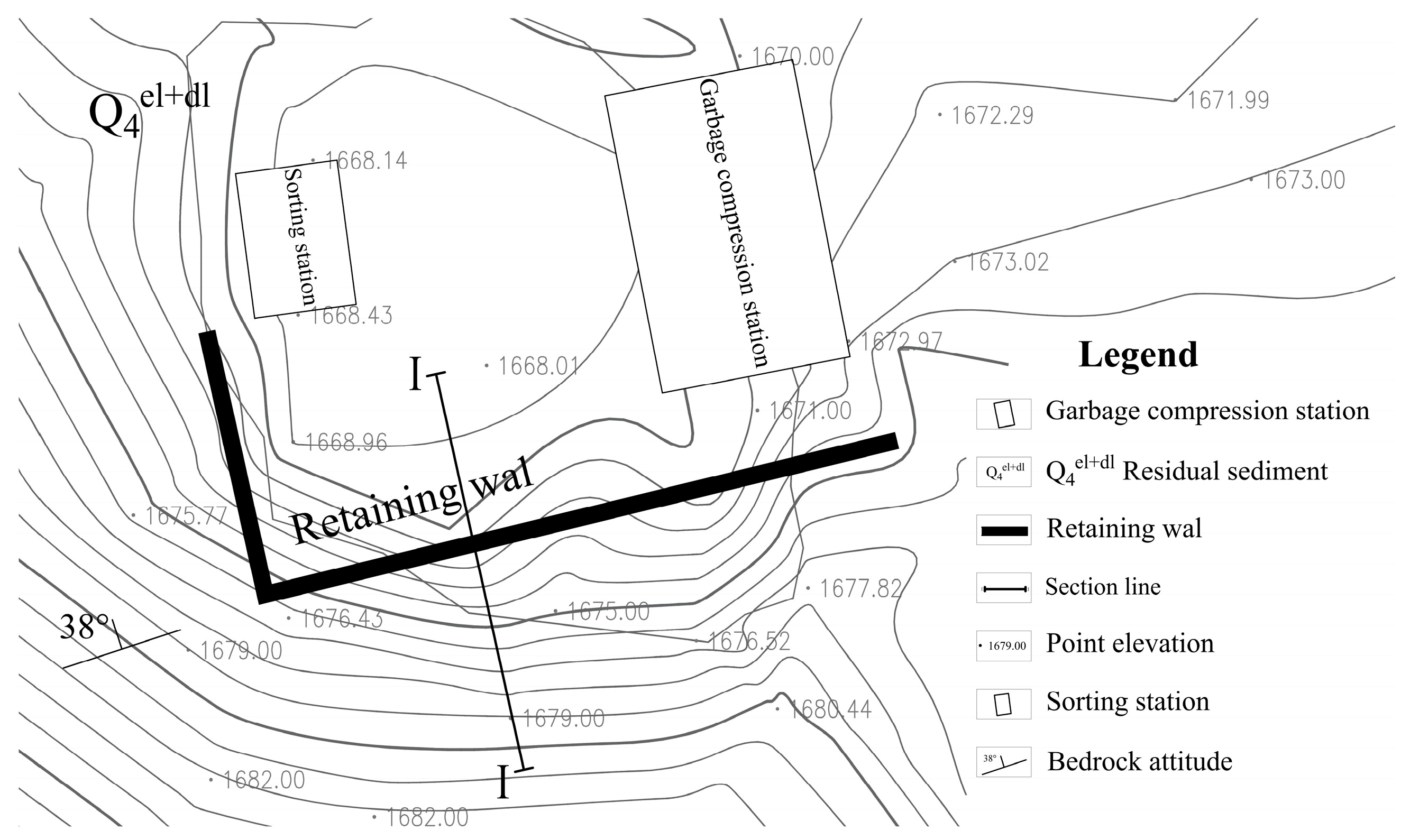
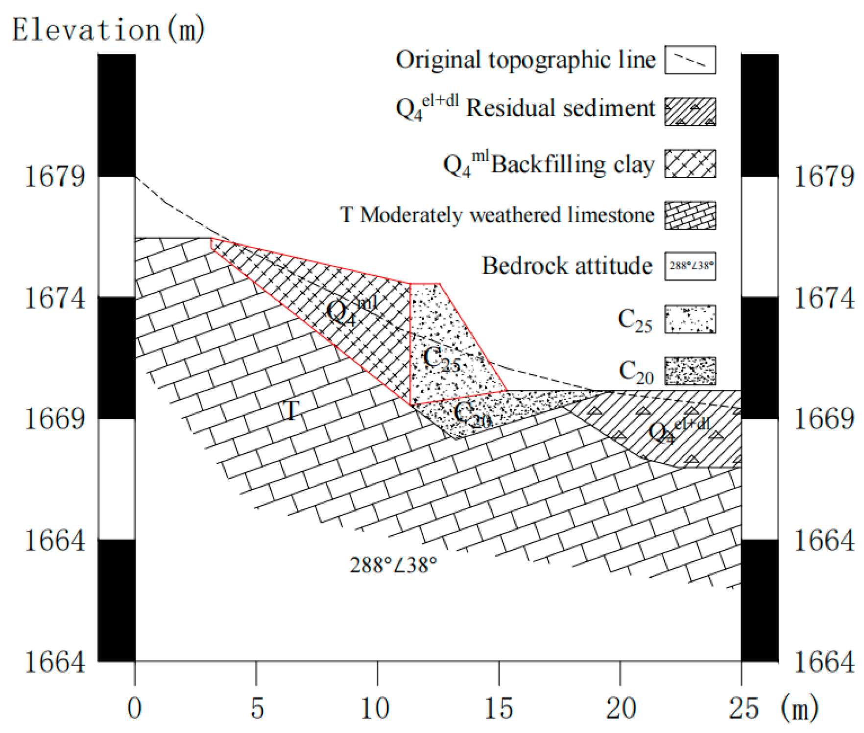
4.2.1. Overview of the Garbage Transfer Station Project
4.2.2. Computational Model
- (1)
- Computation Model Size
- (2)
- Damage Criterion
- (3)
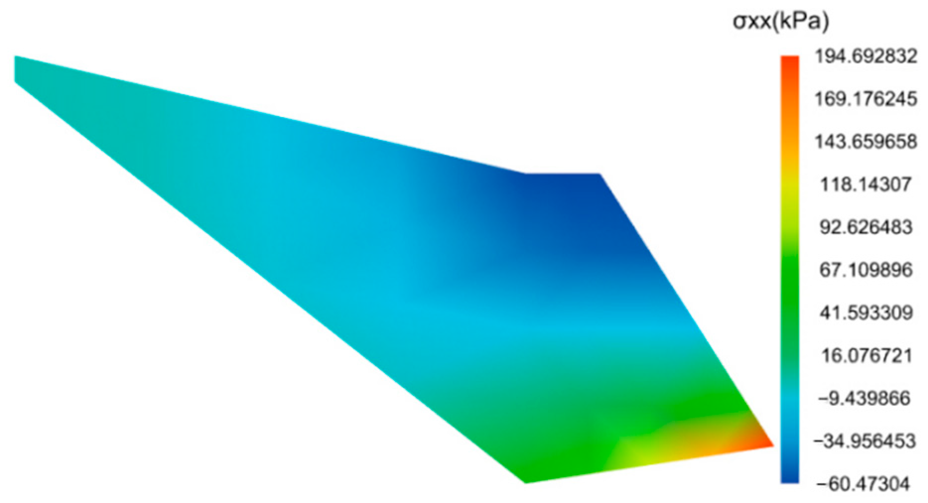
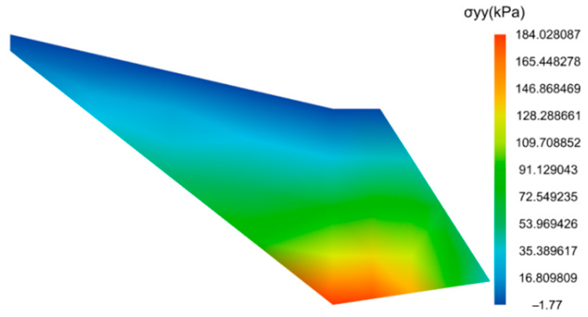
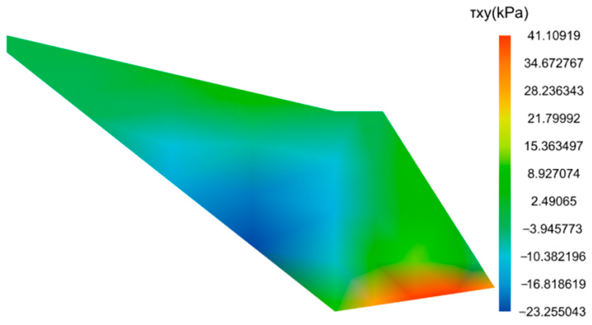
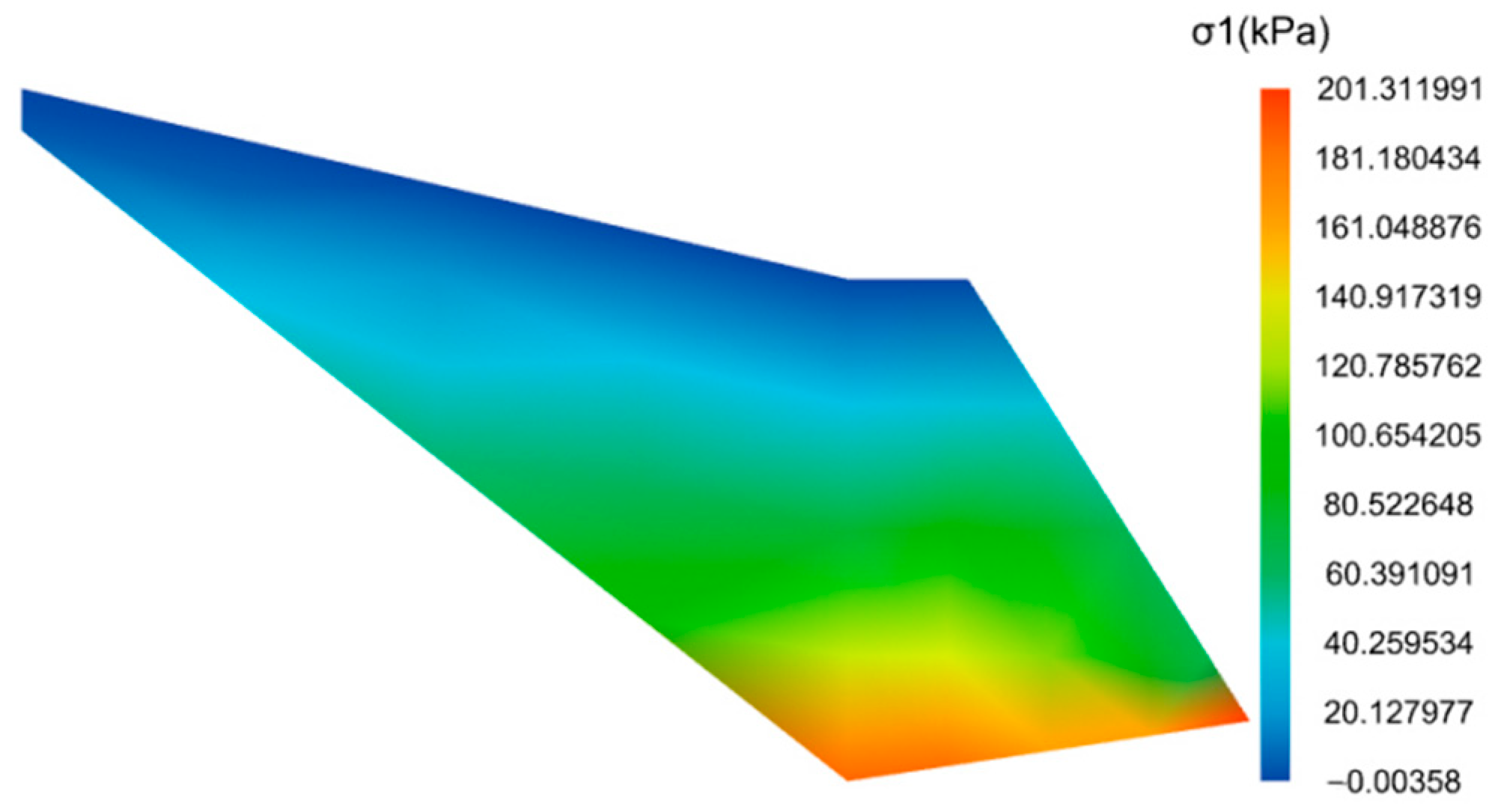
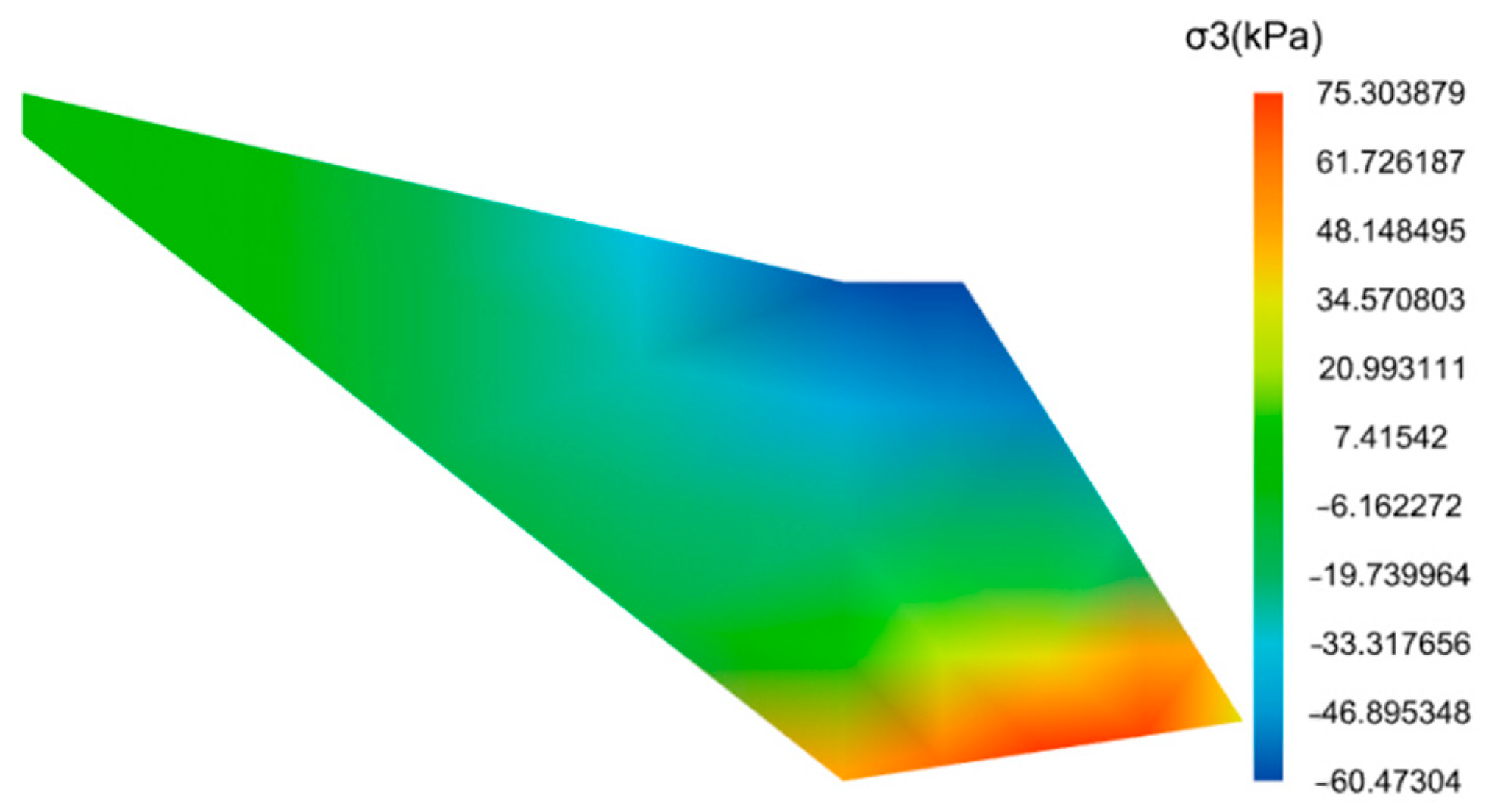
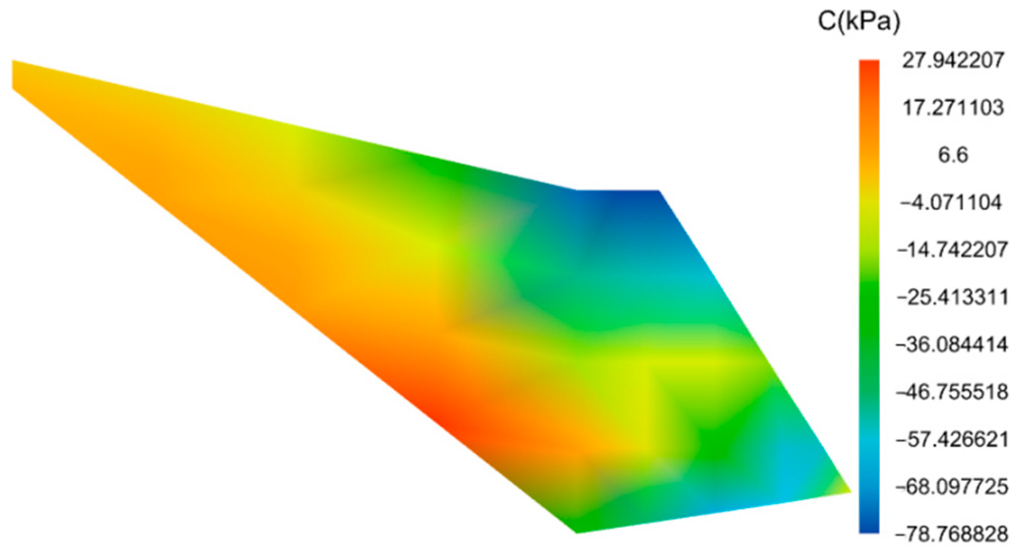
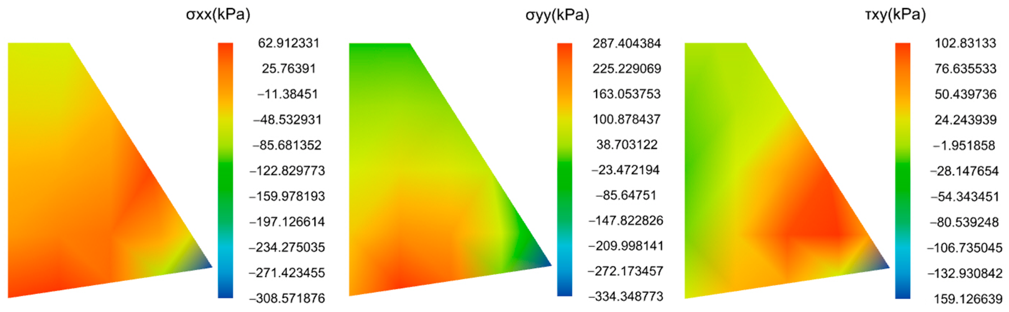
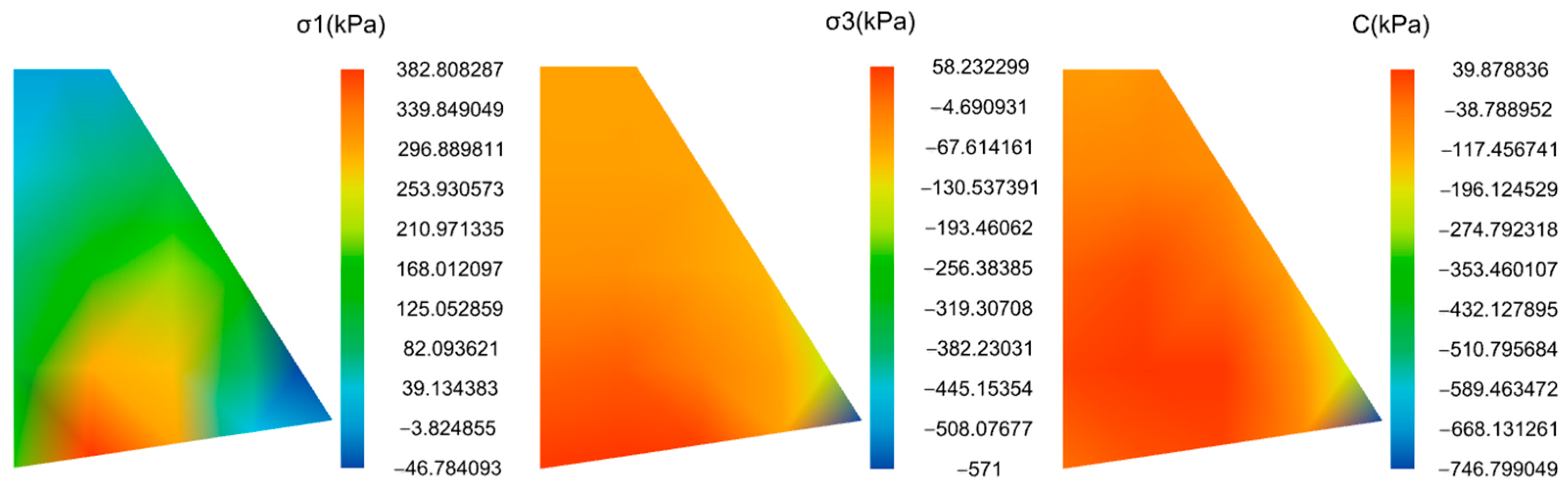
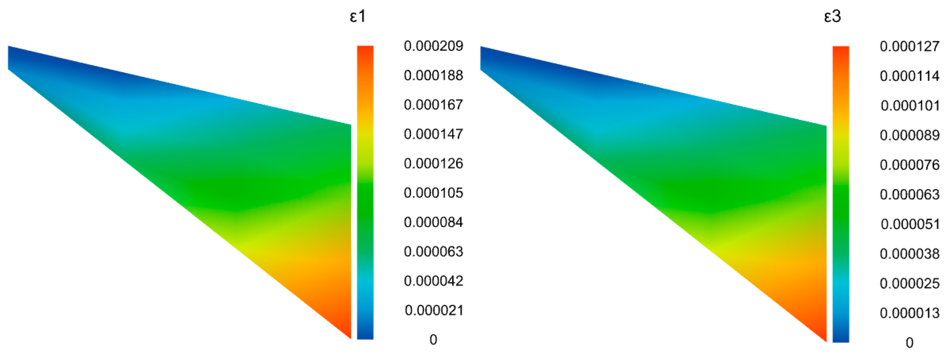
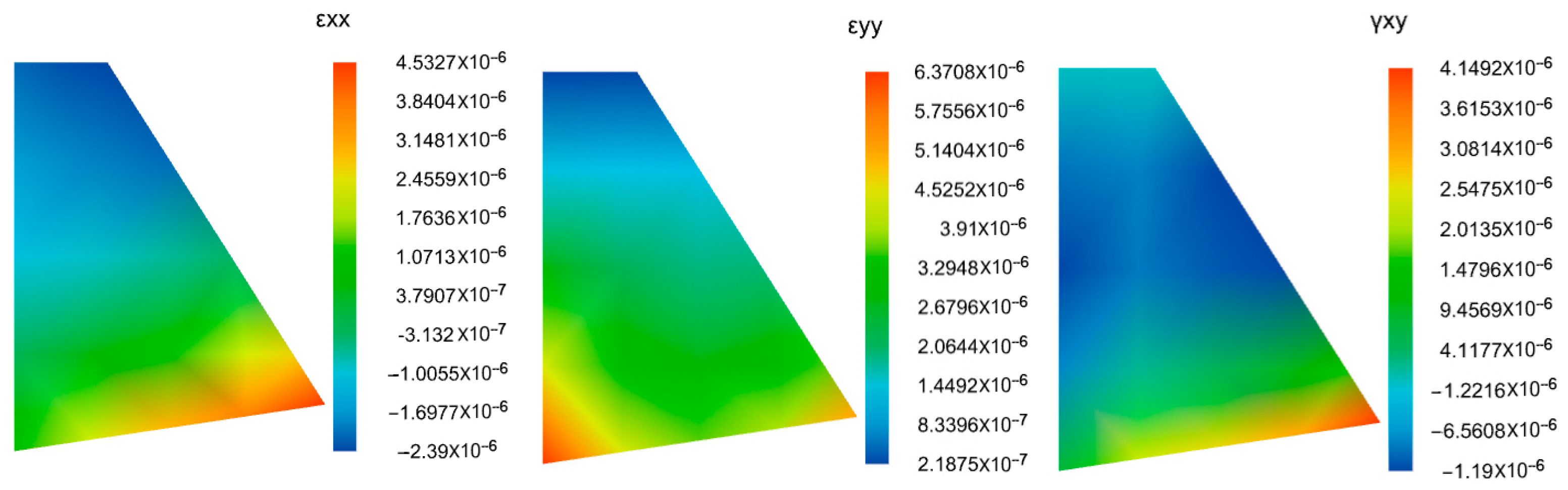
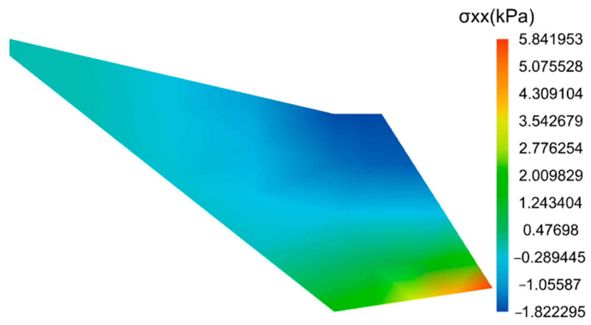
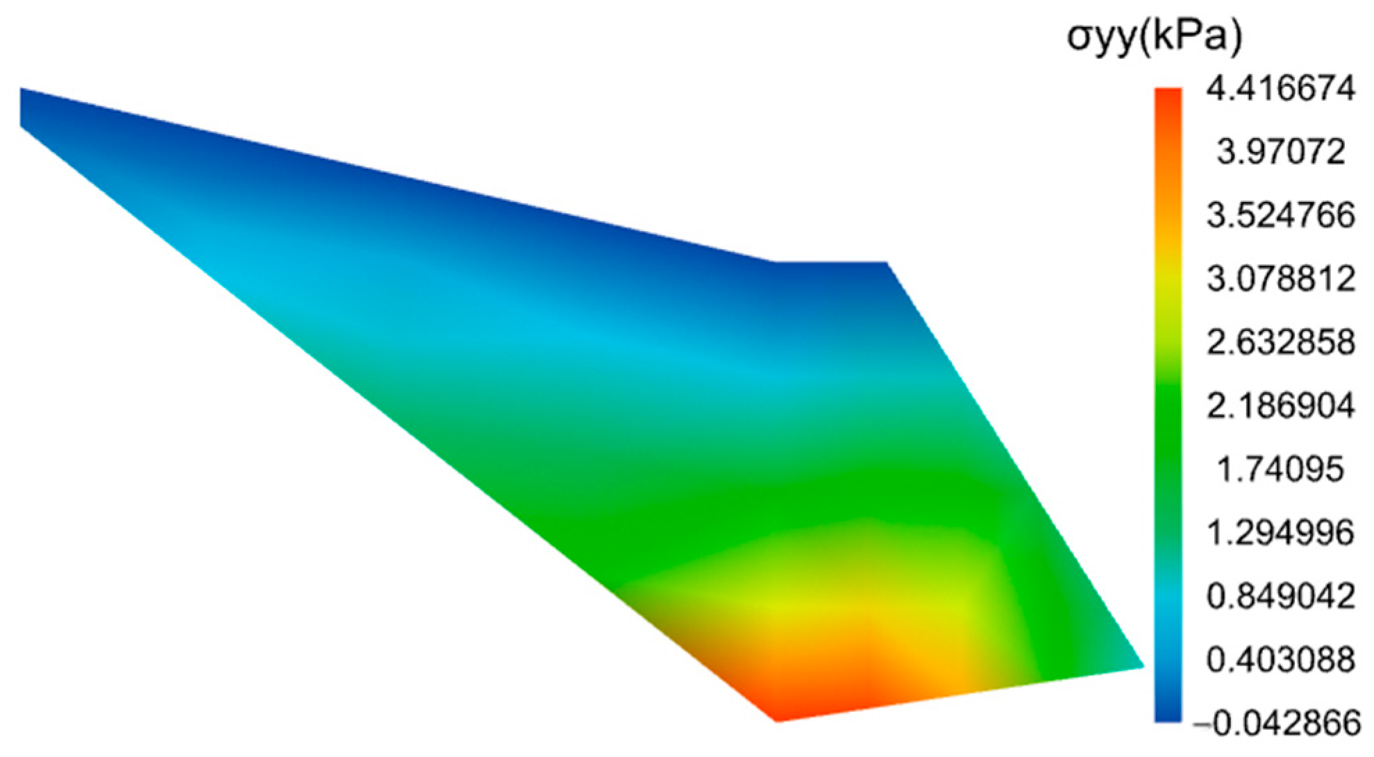
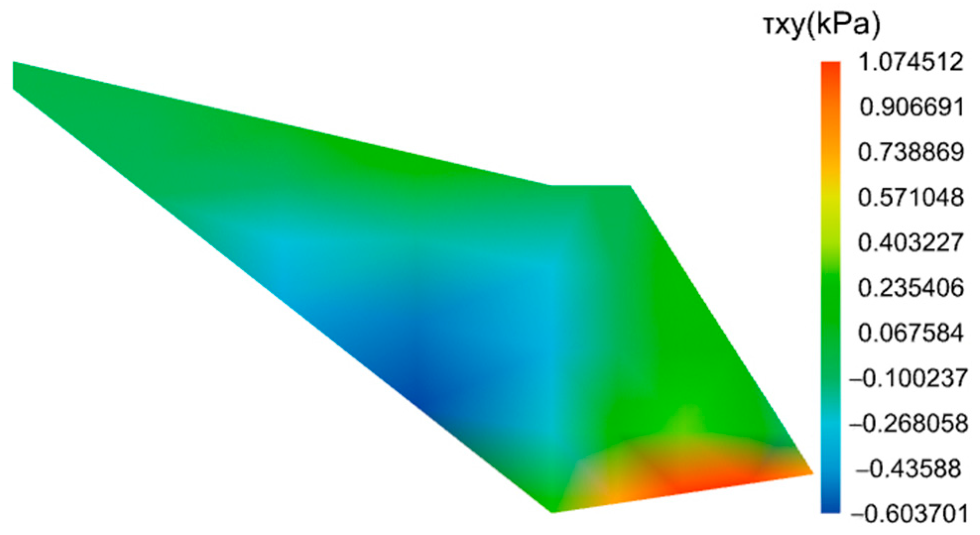
- Computation Results
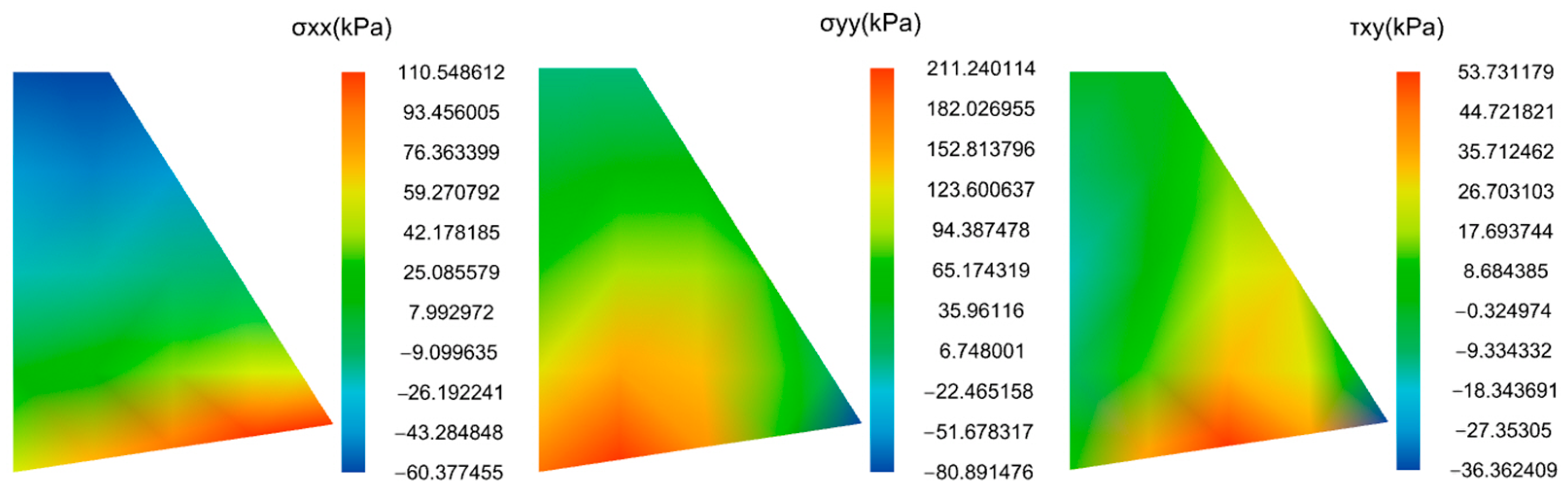
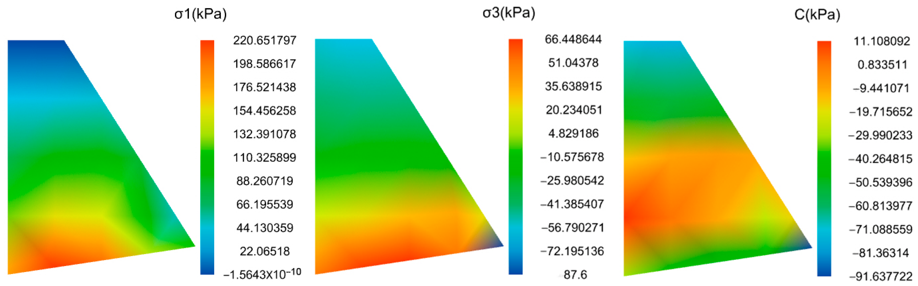
4.2.3. Model Comparison
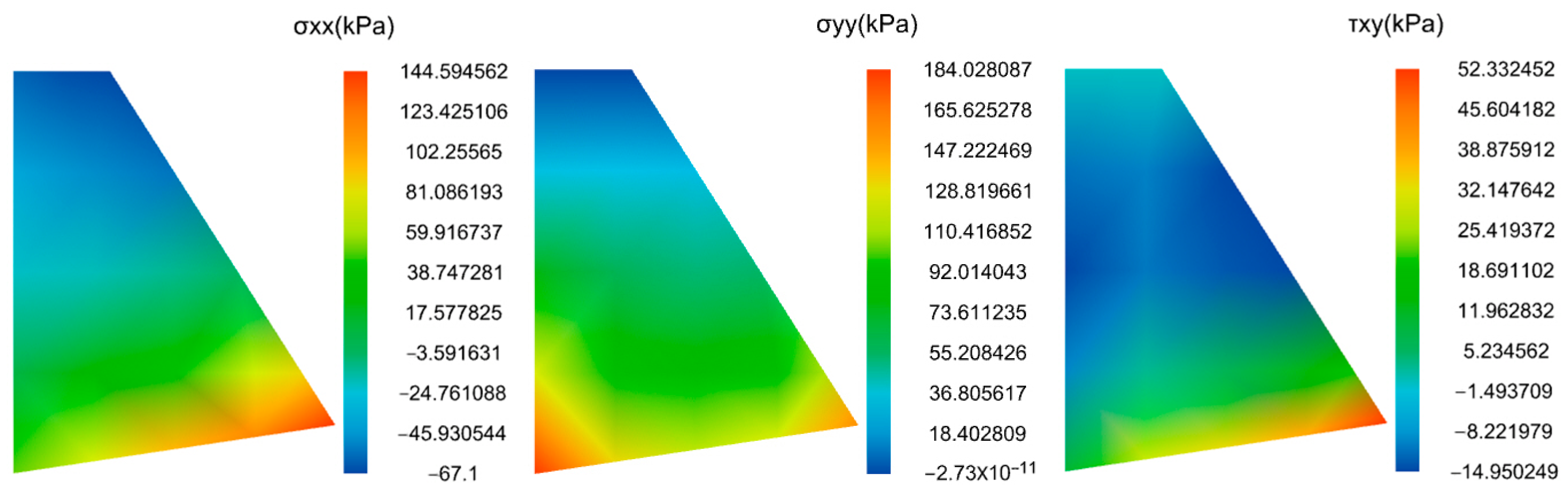
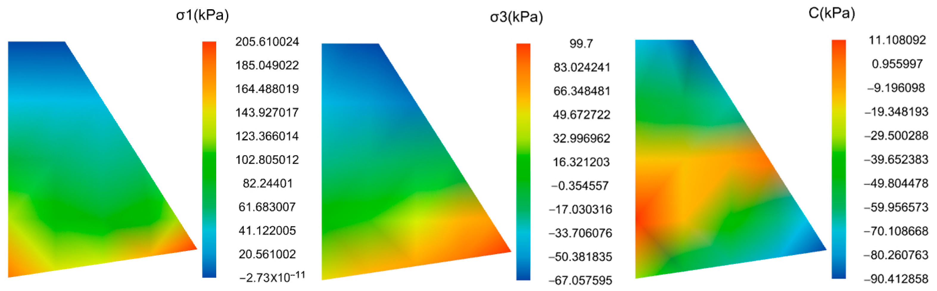
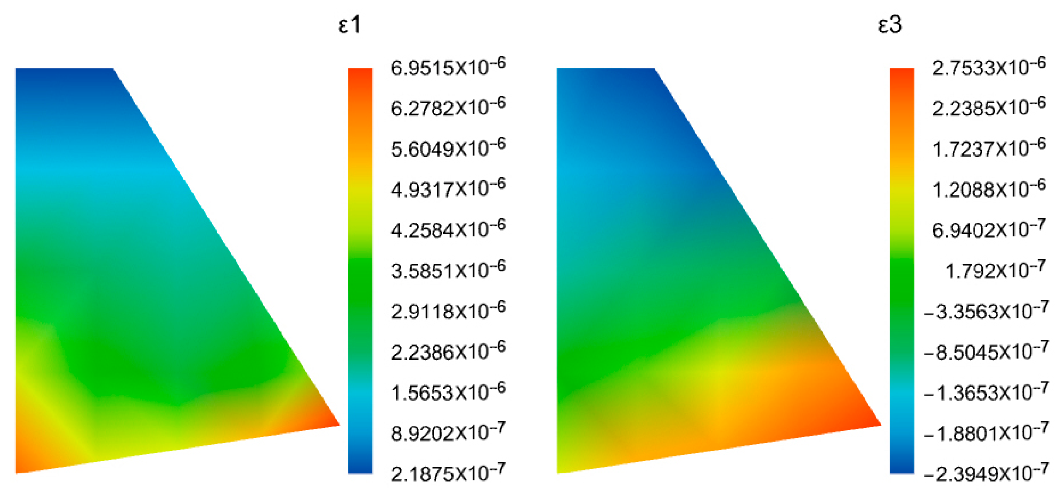
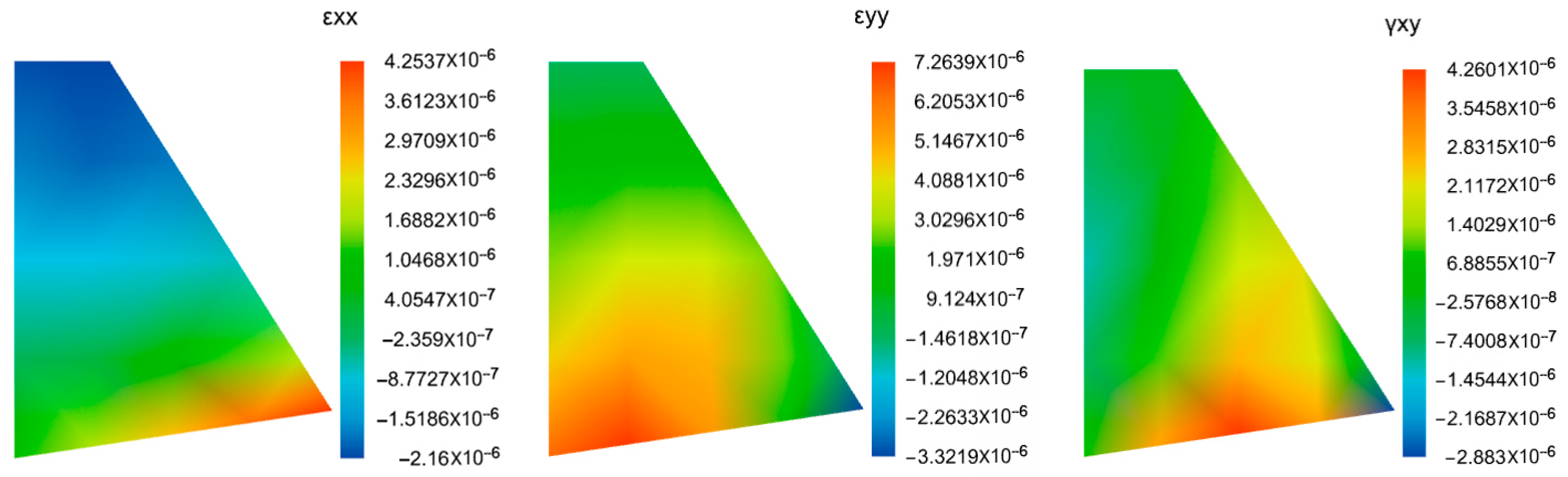
4.3. Analysis of the Calculation Results
4.3.1. Analysis of Soil Wedge Results
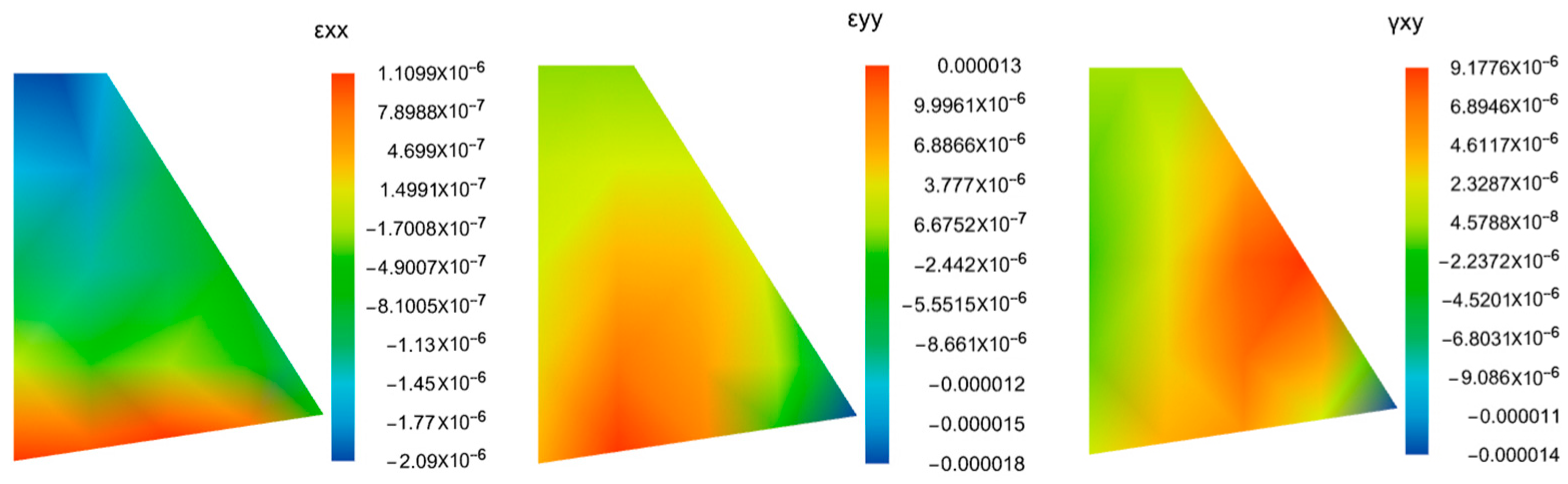
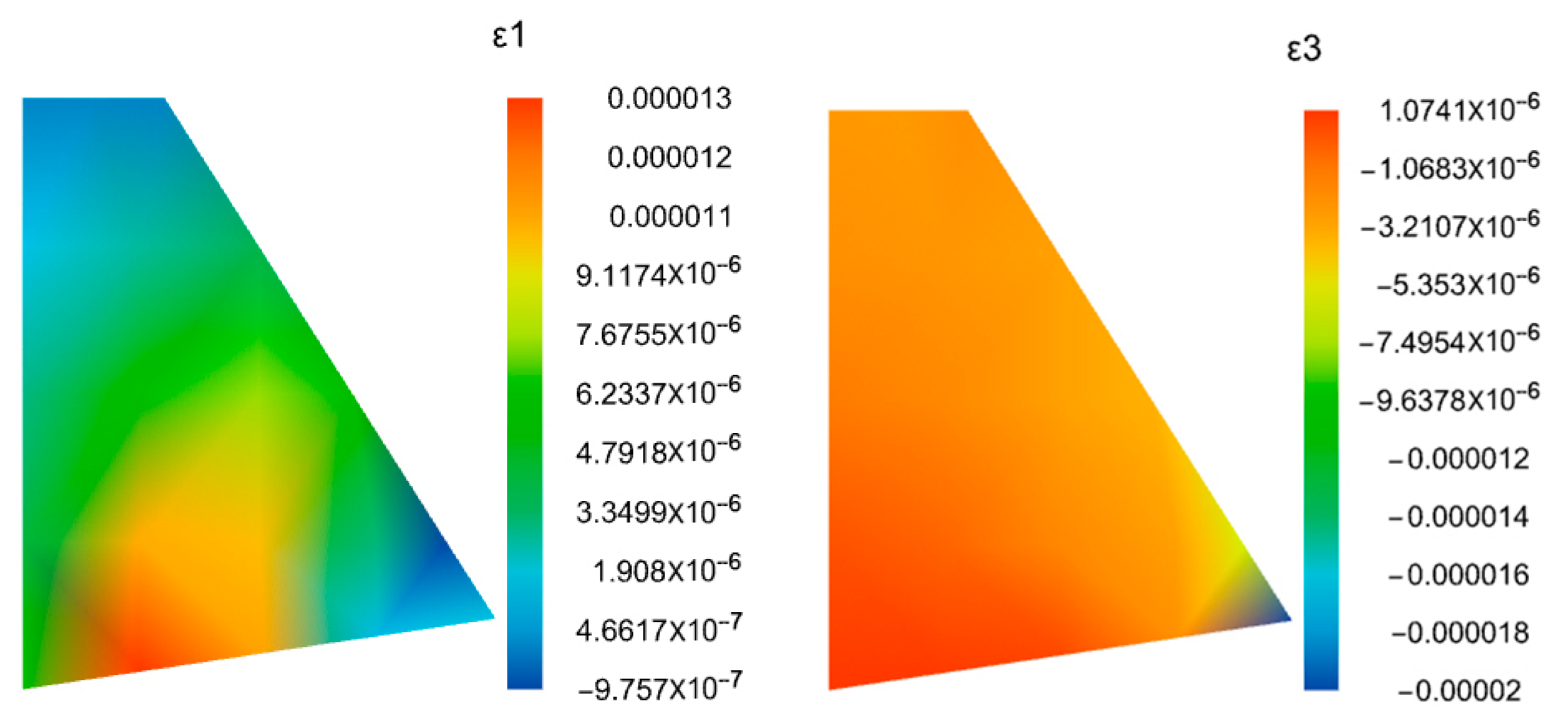
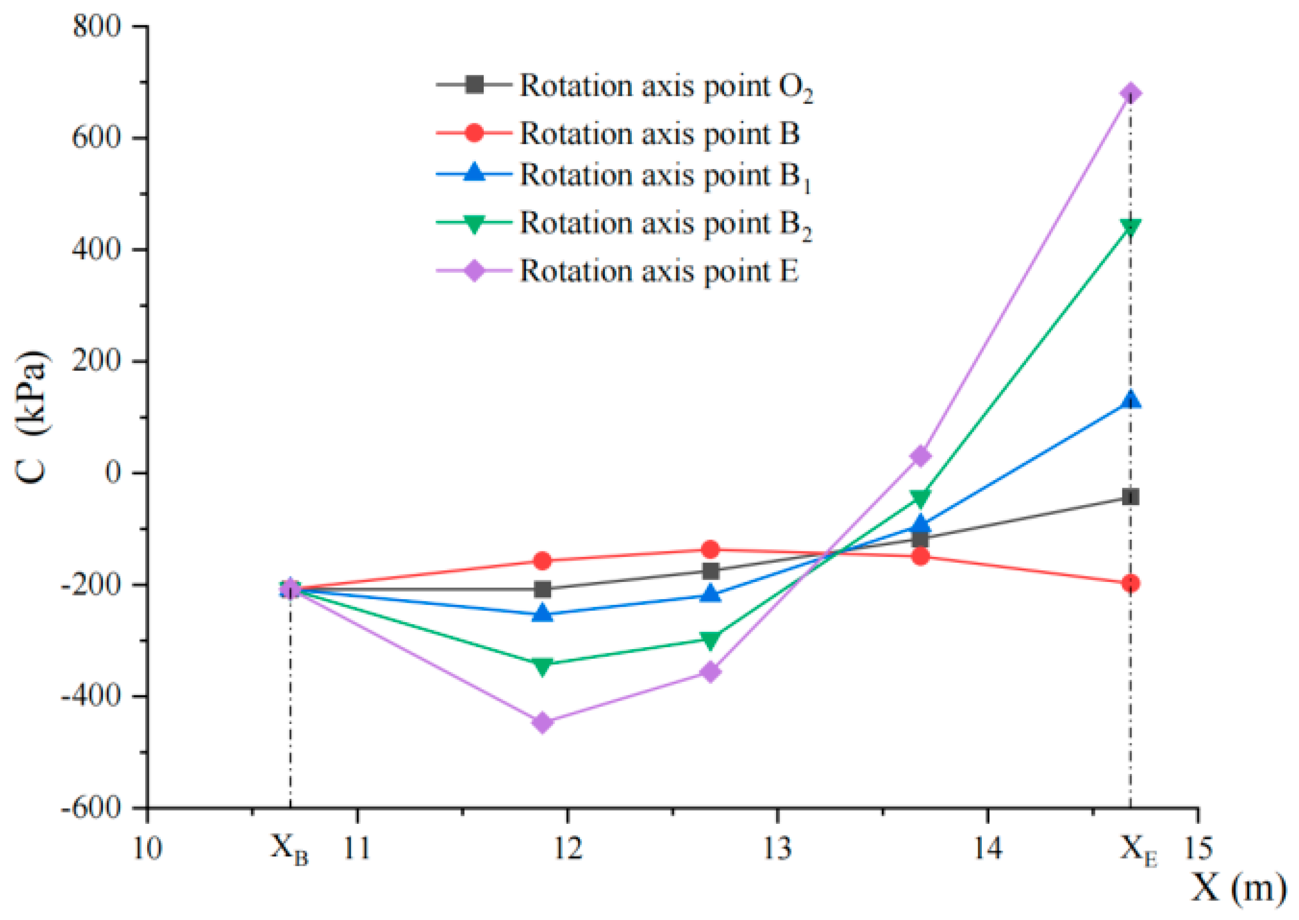
4.3.2. Retaining Wall Stability Analysis
4.4. Discussion
- (1)
- The actual geological conditions of slope engineering are complex, and analyzing and studying only from a two-dimensional plane perspective may result in theoretical calculation results that deviate from the actual situation. Therefore, to fit the actual situation, it is necessary to establish corresponding three-dimensional models to study the corresponding boundary conditions and stress expressions. Further research is needed on the issues of three-dimensional soil wedges and retaining walls
- (2)
- In addition, the theoretical solution calculation method in this study assumes that the research object is a continuous homogeneous medium, and stress continuity is assumed during the solution process. In practical engineering, the parameters of soil wedges and retaining walls are complex and diverse, and factors, such as the position of the slip surface, rainfall, and groundwater seepage, can affect the calculation results. Therefore, establishing a model that considers discontinuous materials is the next direction of this theoretical calculation method.
5. Conclusions
- (1)
- The proposed numerical method can account for different boundary conditions and rotation axes, and the calculated stress and strain have a non-linear relationship with the coordinates.
- (2)
- The proposed numerical theoretical solution, which satisfies the stress differential equations, compatibility equations, and boundary conditions, is capable of obtaining stress distributions at different points. The strain distribution in any direction within the soil wedge can be determined on the basis of the constitutive relationship between the principal stress and principal strain observed in experiments. Furthermore, by applying the current strength criterion, the location of the initial failure can be identified, thereby supporting the application of the point strength design criterion.
- (3)
- The proposed numerical method demonstrates that the solutions vary under different working conditions, allowing the most unfavorable conditions to be identified. Consequently, controlling the rotation point is essential in the design of retaining walls. In addition, the calculation method provides a theoretical basis for the anti-sliding design of retaining walls and other structures and establishes a foundation for slope control and monitoring. Furthermore, new control and prevention methods can be developed on the basis of the form of control and the materials used.
- (4)
- The numerical calculation results were compared with the finite element calculation results, revealing a small deviation of less than 5.05% between the two. The case study demonstrates that the proposed method can be widely applied in engineering practice, including dynamic and static loading and unloading analyses, as well as failure process investigations of roadbeds, tunnels, and dams.
Author Contributions
Funding
Data Availability Statement
Acknowledgments
Conflicts of Interest
Abbreviations
| DOAJ | Directory of Open Access Journals |
| TLA | Three letter acronym |
| LD | Linear dichroism |
References
- Editorial Department of China Journal of Highways. A Review of Academic Research on Chinese Roadbed Engineering 2021. Chin. J. Highw. 2021, 34, 1–49. [Google Scholar] [CrossRef]
- Pei, Z.; Nian, T.; Wu, H.; Zhang, J.; Zhang, C.; Wang, R. Research progress on emergency response technology for landslide geological disasters. J. Disaster Prev. Reduct. Eng. 2021, 41, 1382–1394. [Google Scholar] [CrossRef]
- Xiao, Y. Discussion on the Design of Retaining Walls for Mountainous Highways. Eng. Constr. Des. 2021, 3, 82–84. [Google Scholar] [CrossRef]
- Zhao, L.; Zhong, Z.; Zhao, B.; Zeng, Z.; Gong, X.; Hu, S. Analysis of the Active Earth Pressure of Sandy Soil under the Translational Failure Mode of Rigid Retaining Walls Near Slopes. KSCE J. Civ. Eng. 2024, 28, 5500–5515. [Google Scholar] [CrossRef]
- Li, Z.W.; Yang, X.L.; Li, Y.X. Active earth pressure coefficients based on a 3D rotational mechanism. Comput. Geotech. 2019, 112, 342–349. [Google Scholar] [CrossRef]
- Zhang, Z.L.; Zhu, J.Q.; Yang, X.L. Three-dimensional active earth pressures for unsaturated backfills with cracks considering steady seepage. Int. J. Geomech. 2023, 23, 04022270. [Google Scholar] [CrossRef]
- Que, Y.; Long, C.; Chen, F. Seismic active earth pressure of infinite width backfilled soil on cantilever retaining wall with long relief shelf under translational mode. KSCE J. Civ. Eng. 2023, 27, 3285–3299. [Google Scholar] [CrossRef]
- Zhou, Y.; Chen, Y. Active and Passive Earth Pressure Calculation Method for Double-Row Piles considering the Nonlinear Pile Deformation. Geofluids 2022, 2022, 4061624. [Google Scholar] [CrossRef]
- Chen, Y.; Li, B. Research on the Calculation of Soil Pressure on Retaining Walls. Transp. Technol. Manag. 2023, 4, 90–92. [Google Scholar]
- Lai, F.; Zhang, N.; Liu, S.; Yang, D. A generalised analytical framework for active earth pressure on retaining walls with narrow soil. Géotechnique 2022, 74, 1127–1142. [Google Scholar] [CrossRef]
- Yang, D.; Lai, F.; Liu, S. Earth pressure in narrow cohesive-fictional soils behind retaining walls rotated about the top: An analytical approach. Comput. Geotech. 2022, 149, 104849. [Google Scholar] [CrossRef]
- Cao, W.; Zhang, H.; Liu, T.; Tan, X. Analytical solution for the active earth pressure of cohesionless soil behind an inclined retaining wall based on the curved thin-layer element method. Comput. Geotech. 2020, 128, 103851. [Google Scholar] [CrossRef]
- Chen, R.P.; Xu, Y.; Wang, H.L.; Meng, F. Theoretical model of lateral soil arching effect in sand with flexible retaining wall. Proc. Inst. Civ. Eng.-Geotech. Eng. 2025, 1–16. [Google Scholar] [CrossRef]
- Gong, Q.; Muho, E.V.; Beskou, N.D.; Zhou, Y. Approximate analytical/numerical solutions for the seismic response of rigid walls retaining a transversely isotropic poroelastic soil. Adv. Eng. Softw. 2025, 202, 103876. [Google Scholar] [CrossRef]
- Que, Y.; Zhang, J.; Tian, Y.; Li, X. Spatial earth pressure analysis of clayey fill behind retaining wall in V-shaped gully terrain. Soils Found. 2024, 64, 101538. [Google Scholar] [CrossRef]
- Chen, H.B.; Shao, X.Y.; Han, L.; Li, M.G.; Chen, F.Q.; Xie, X.L. A comprehensive prediction of stability against cantilever retaining walls using finite element limit analysis and neural networks model. KSCE J. Civ. Eng. 2025, 100200. [Google Scholar] [CrossRef]
- Yang, T.; Huang, G.; Xie, J.; Ji, L.; Wu, H. Calculation method of point safety factor for landslide stability analysis. J. Eng. Geol. 2014, 1–10. [Google Scholar] [CrossRef]
- Li, Z.; Xiao, S. Calculation method for seismic active earth pressure of cantilever retaining wall. J. Geotech. Eng. 2023, 45, 196–205. [Google Scholar]
- Rui, R.; Jiang, W.; Xu, Y.; Xia, R.; Emmanuel, E.E.; Ding, R. Experimental study on the influence of displacement mode of rigid retaining wall on soil pressure. J. Rock Mech. Eng. 2023, 42, 1534–1545. [Google Scholar] [CrossRef]
- Deng, B.; Yang, M.; Wang, D.; Fan, J. Failure mode and active soil pressure calculation of unsaturated soil behind rigid retaining wall. Geotech. Mech. 2022, 43, 2371–2382. [Google Scholar] [CrossRef]
- Du, H.; Song, L.; Liu, J.; Bai, Q. Calculation method for soil pressure of gravity reinforced soil retaining wall. J. Shihezi Univ. (Nat. Sci. Ed.) 2023, 41, 291–297. [Google Scholar] [CrossRef]
- Dang, F.; Zhang, L.; Wang, X.; Ding, J.; Gao, J. Analysis of soil pressure on retaining walls under finite displacement conditions based on elastic theory. J. Rock Mech. Eng. 2020, 39, 2094–2103. [Google Scholar] [CrossRef]
- Lu, Y.F. Deformation and failure mechanism of slope in three dimensions. J. Rock Mech. Geotech. Eng. 2015, 7, 109–119. [Google Scholar] [CrossRef]
- Zhang, Y.F.; Lu, Y.F.; Zhong, Y.; Li, J.; Liu, D.Z. Stability analysis of landfills contained by retaining walls using continuous stress method. CMES-Comput. Model. Eng. Sci. 2023, 134, 357. [Google Scholar] [CrossRef]
- Lu, Y.F.; Sun, W.Q.; Yang, H.; Jiang, J.J.; Lu, L.E. A new calculation method of force and displacement of retaining wall and slope. Appl. Sci. 2023, 13, 5806. [Google Scholar] [CrossRef]
- Lu, Y.; Liu, G.; Cui, K.; Zheng, J. Mechanism and Stability Analysis of Deformation Failure of a Slope. Adv. Civ. Eng. 2021, 2021, 8949846. [Google Scholar] [CrossRef]


| Unit | aij i∈(1,3) | ai,0 | ai,1 | ai,2 | ai,3 | ai,4 | ai,5 | ai,6 | ai,7 | ai,8 | ai,9 | ai,10 | ai,11 | ai,12 | ai,13 | ai,14 | ai,15 | ai,16 | ai,17 | ai,18 | ai,19 | ai,20 |
|---|---|---|---|---|---|---|---|---|---|---|---|---|---|---|---|---|---|---|---|---|---|---|
| kPa | kPa | kPa /m | kPa /m | kPa /m2 | kPa /m2 | kPa /m2 | kPa /m3 | kPa /m3 | kPa /m3 | kPa /m3 | kPa /m4 | kPa /m4 | kPa /m4 | kPa /m4 | kPa /m4 | kPa /m5 | kPa /m5 | kPa /m5 | kPa /m5 | kPa /m5 | kPa /m5 | |
| I | σxx | −8.514589832 | 10.7338006 | 1.975186322 | −4.686005862 | −2.4311721 | −0.081066929 | 0.783697159 | 1.011448983 | 0.098342413 | −6.4374 × 10⁻¹⁵ | −0.035729565 | −0.147801243 | −0.039766443 | 9.34631 × 10⁻¹⁶ | 4.18172 × 10⁻¹⁶ | 0.001208862 | 0.002318841 | 0.005360081 | −1.1252 × 10⁻¹⁶ | −1.12094 × 10⁻¹⁶ | 0− |
| σyy | 289.5878581 | −25.57832168 | −6.284912858 | −6.760674299 | −9.743081267 | −4.686005862 | 1.783788853 | 2.472570175 | 2.351091476 | 0.337149661 | −0.085824316 | −0.30484489 | −0.214377393 | −0.147801243 | −0.00662774 | 0.001113794 | 0.007179218 | 0.01208862 | 0.004637683 | 0.002680041 | −1.1252 × 10⁻¹⁷ | |
| τxy | 12.88274782 | −13.31508714 | −10.7338006 | 4.871540634 | 9.372011724 | 1.21558605 | −0.824190058 | −2.351091476 | −1.011448983 | −0.032780804 | 0.076211222 | 0.142918262 | 0.221701864 | 0.026510962 | −2.33658 × 10⁻¹⁶ | −0.001435844 | −0.00604431 | −0.004637683 | −0.005360081 | 5.626 × 10⁻¹⁷ | 2.24188 × 10⁻¹⁷ | |
| II | σxx | −2231.174997 | −237.6119698 | 3290.591566 | 175.1101396 | −754.6661804 | −455.0088761 | −18.41150807 | 39.32303445 | 127.8870528 | 4.89176 × 10⁻¹³ | 0.499646849 | 1.664172127 | −12.0050015 | −2.12887 × 10⁻¹³ | 5.07007 × 10⁻¹⁶ | 0.00685827 | −0.13849182 | 0.378806868 | 5.78534 × 10⁻¹⁵ | 2.40638 × 10⁻¹⁶ | 0 |
| σyy | −4074.640752 | 1346.14285 | −729.6690351 | −142.4134669 | 75.15955343 | 175.1101396 | 5.264073151 | 11.25086603 | −55.23452421 | 13.10767815 | 1.36445 × 10⁻³⁰ | −1.201706004 | 2.997881096 | 1.664172127 | −2.000833584 | 0 | 9.21839 × 1031 | 0.068582696 | −0.276983641 | 0.189403434 | 5.78534 × 10⁻¹⁶ | |
| τxy | −2378.01372 | 704.6690351 | 237.6119698 | −37.57977672 | −350.2202793 | 377.3330902 | −3.750288675 | 55.23452421 | −39.32303445 | −42.62901762 | 0.300426501 | −1.998587397 | −2.49625819 | 8.003334335 | 5.32217 × 10⁻¹⁴ | −1.84368 × 10⁻³¹ | −0.034291348 | 0.276983641 | −0.378806868 | −2.89267 × 10⁻¹⁵ | −4.81276 × 10⁻¹⁷ |
| Unit | aij i∈(1,3) | ai,0 | ai,1 | ai,2 | ai,3 | ai,4 | ai,5 | ai,6 | ai,7 | ai,8 | ai,9 | ai,10 | ai,11 | ai,12 | ai,13 | ai,14 | ai,15 | ai,16 | ai,17 | ai,18 | ai,19 | ai,20 |
|---|---|---|---|---|---|---|---|---|---|---|---|---|---|---|---|---|---|---|---|---|---|---|
| kPa | kPa | kPa /m | kPa /m | kPa /m2 | kPa /m2 | kPa /m2 | kPa /m3 | kPa /m3 | kPa /m3 | kPa /m3 | kPa /m4 | kPa /m4 | kPa /m4 | kPa /m4 | kPa /m4 | kPa /m5 | kPa /m5 | kPa /m5 | kPa /m5 | kPa /m5 | kPa /m5 | |
| B | σxx | 1057.401297 | 12.93321823 | −901.7984207 | −60.84710546 | 197.8176225 | 151.0830504 | 7.693568789 | −7.697202933 | −42.3634883 | 5.15296 × 10⁻¹³ | −0.269465065 | −0.816186191 | 3.936060403 | 1.58737 × 10⁻¹⁴ | −5.39781 × 10⁻¹⁵ | 0.000776367 | 0.046335254 | −0.118729396 | −4.58553 × 10⁻¹⁶ | 7.72726 × 10⁻¹⁶ | 0 |
| σyy | 3692.385668 | −375.3434249 | −132.5773924 | 0.535922331 | −56.80117939 | −60.84710546 | 0.595901458 | 6.990593268 | 23.08070637 | −2.565734311 | 0 | −0.136035032 | −1.616790393 | −0.816186191 | 0.656010067 | 0 | −2.55018 × 10⁻³¹ | 0.00776367 | 0.092670507 | −0.059364698 | −4.58553 × 10⁻¹⁷ | |
| τxy | −1790.733007 | 107.5773924 | −12.93321823 | 28.40058969 | 121.6942109 | −98.90881127 | −2.330197756 | −23.08070637 | 7.697202933 | 14.12116277 | 0.034008758 | 1.077860262 | 1.224279287 | −2.624040269 | −3.96841 × 10⁻¹⁵ | 5.10036 × 10⁻³² | −0.003881835 | −0.092670507 | 0.118729396 | 2.29276 × 10⁻¹⁶ | −1.54545 × 10⁻¹⁶ | |
| B1 | σxx | −2681.606157 | 550.3246785 | 1547.407161 | −8.249911582 | −384.2406183 | −217.9893666 | −4.65598325 | 26.96726623 | 61.30853894 | −8.75072 × 10⁻¹³ | 0.332192276 | −0.040854443 | −5.771058252 | 1.28719 × 10⁻¹³ | 1.12857 × 10⁻¹⁴ | −0.004861229 | −0.040614373 | 0.184239351 | 9.45318 × 10⁻¹⁶ | −1.00888 × 10⁻¹⁵ | 0 |
| σyy | −5324.401451 | 501.0704196 | 636.8507964 | 43.73994808 | 6.369680178 | −8.249911582 | −3.73124213 | −16.21987184 | −13.96794975 | 8.989088744 | 0 | 0.851784529 | 1.993153658 | −0.040854443 | −0.961843042 | 0 | 0 | −0.048612289 | −0.081228745 | 0.092119676 | 9.45318 × 10⁻¹⁷ | |
| τxy | 3817.518942 | −661.8507964 | −550.3246785 | −3.184840089 | 16.49982316 | 192.1203092 | 5.406623947 | 13.96794975 | −26.96726623 | −20.43617965 | −0.212946132 | −1.328769105 | 0.061281665 | 3.847372168 | −3.21797 × 10⁻¹⁴ | 0 | 0.024306145 | 0.081228745 | −0.184239351 | −4.72659 × 10⁻¹⁶ | 2.01776 × 10⁻¹⁶ | |
| B2 | σxx | 68517.8476 | −18838.22679 | −22807.23254 | 1711.192052 | 6361.895361 | 1680.440889 | −52.22439244 | −586.892854 | −471.9583868 | 6.99976 × 10⁻¹² | 0.317204083 | 17.45160699 | 44.16030183 | −4.44711 × 10⁻¹³ | −9.1815 × 10⁻¹⁴ | −0.02005534 | 0.037415513 | −1.374167643 | 3.45636 × 10⁻¹⁴ | −2.338 × 10⁻¹⁴ | 0 |
| σyy | −1461.054204 | −698.2970009 | −4758.585968 | 246.7227145 | 574.8492968 | 1711.192052 | −15.39350032 | −50.5792929 | −156.6731773 | −195.6309513 | −1.02007 × 10⁻³¹ | 3.514096637 | 1.903224499 | 17.45160699 | 7.360050305 | 0 | 1.1157 × 10⁻³² | −0.200553398 | 0.074831025 | −0.687083821 | 3.45636 × 10⁻¹⁵ | |
| τxy | −26677.40723 | 4733.585968 | 18838.22679 | −287.4246484 | −3422.384104 | −3180.947681 | 16.8597643 | 156.6731773 | 586.892854 | 157.3194623 | −0.878524159 | −1.268816333 | −26.17741048 | −29.44020122 | 1.11178 × 10⁻¹³ | −2.23141 × 10⁻³³ | 0.100276699 | −0.074831025 | 1.374167643 | −1.72818 × 10⁻¹⁴ | 4.67601 × 10⁻¹⁵ | |
| E | σxx | 33048.3391 | −10789.38026 | −6035.154863 | 1259.831626 | 2202.733342 | −279.2975565 | −57.66300158 | −300.8469261 | 78.5299406 | −1.43625 × 10⁻¹¹ | 0.409520591 | 18.20442305 | −7.383549045 | 2.22108 × 10⁻¹⁴ | −1.08313 × 10⁻¹³ | 0.026114474 | −0.415795704 | 0.234566779 | −2.46143 × 10⁻¹⁴ | −1.94125 × 10⁻¹⁵ | 0 |
| σyy | −59701.97769 | 13278.26737 | 4301.825456 | −929.8131553 | −1476.204359 | 1259.831626 | 20.04419616 | 148.4329786 | −172.9890047 | −100.2823087 | −1.18032 × 10⁻³⁰ | −4.575778143 | 2.457123548 | 18.20442305 | −1.230591507 | 0 | 1.00948 × 10⁻³¹ | 0.26114474 | −0.831591408 | 0.11728339 | −2.46143 × 10⁻¹⁵ | |
| τxy | 7612.300053 | −4326.825456 | 10789.38026 | 738.1021796 | −2519.663252 | −1101.366671 | −49.47765953 | 172.9890047 | 300.8469261 | −26.17664687 | 1.143944536 | −1.638082365 | −27.30663457 | 4.92236603 | −5.5527 × 10⁻¹⁵ | −2.01896 × 10⁻³² | −0.13057237 | 0.831591408 | −0.234566779 | 1.23072 × 10⁻¹⁴ | 3.88249 × 10⁻¹⁶ |
Disclaimer/Publisher’s Note: The statements, opinions and data contained in all publications are solely those of the individual author(s) and contributor(s) and not of MDPI and/or the editor(s). MDPI and/or the editor(s) disclaim responsibility for any injury to people or property resulting from any ideas, methods, instructions or products referred to in the content. |
© 2025 by the authors. Licensee MDPI, Basel, Switzerland. This article is an open access article distributed under the terms and conditions of the Creative Commons Attribution (CC BY) license (https://creativecommons.org/licenses/by/4.0/).
Share and Cite
Zhang, S.; Lu, Y.; Lu, L. A New Method for Evaluating the Stability of Retaining Walls. Buildings 2025, 15, 1732. https://doi.org/10.3390/buildings15101732
Zhang S, Lu Y, Lu L. A New Method for Evaluating the Stability of Retaining Walls. Buildings. 2025; 15(10):1732. https://doi.org/10.3390/buildings15101732
Chicago/Turabian StyleZhang, Shiqi, Yingfa Lu, and Lier Lu. 2025. "A New Method for Evaluating the Stability of Retaining Walls" Buildings 15, no. 10: 1732. https://doi.org/10.3390/buildings15101732
APA StyleZhang, S., Lu, Y., & Lu, L. (2025). A New Method for Evaluating the Stability of Retaining Walls. Buildings, 15(10), 1732. https://doi.org/10.3390/buildings15101732