
Developing an Artificial Neural Network-Based Grading Model for Energy Consumption in Residential Buildings
 ,
,  ,
,  ,
, 

Abstract
1. Introduction
2. Methodology
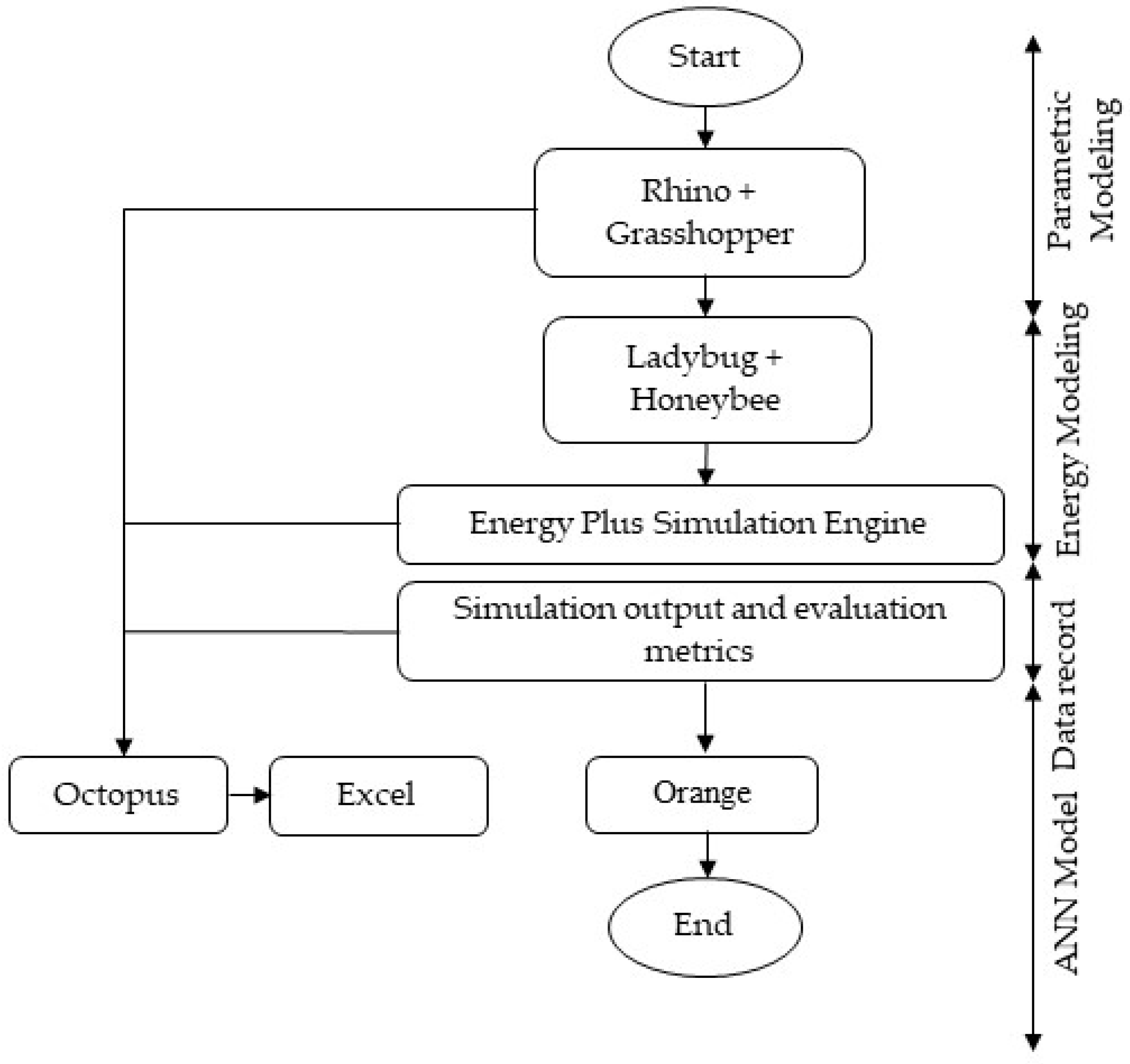
2.1. Computational Framework
2.2. Energy Modeling and Simulation of Existing Samples
2.2.1. Weather Data
2.2.2. Simulation Input Parameters
2.2.3. Energy Simulation Workflow
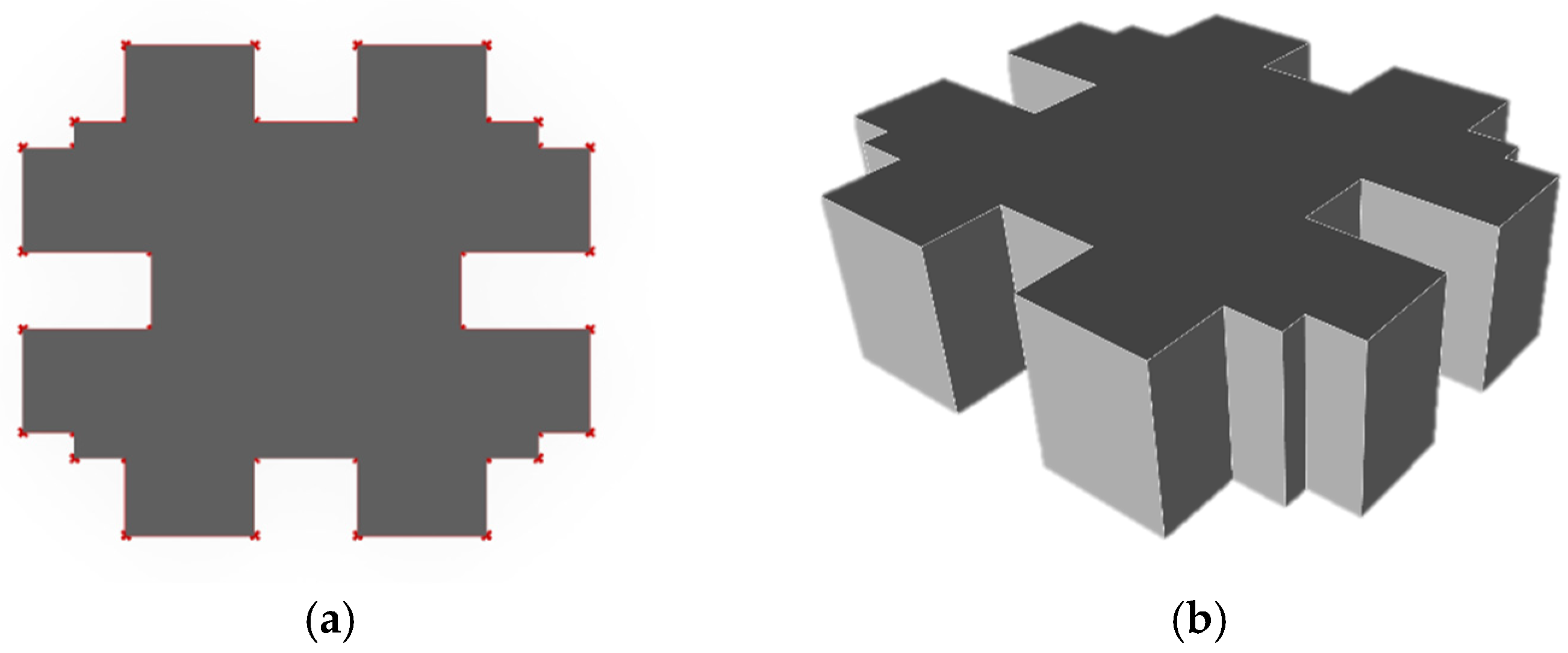
2.3. Proposed Parametric Model
2.3.1. Simulation Variables
2.3.2. Modeling and Energy Simulation Workflow
2.3.3. Validation of Results
2.4. AI Model Development
2.4.1. Data Preprocessing
2.4.2. Model Selection
2.4.3. ANN Model Architecture
2.4.4. Energy Consumption Grading Using KNN
3. Results
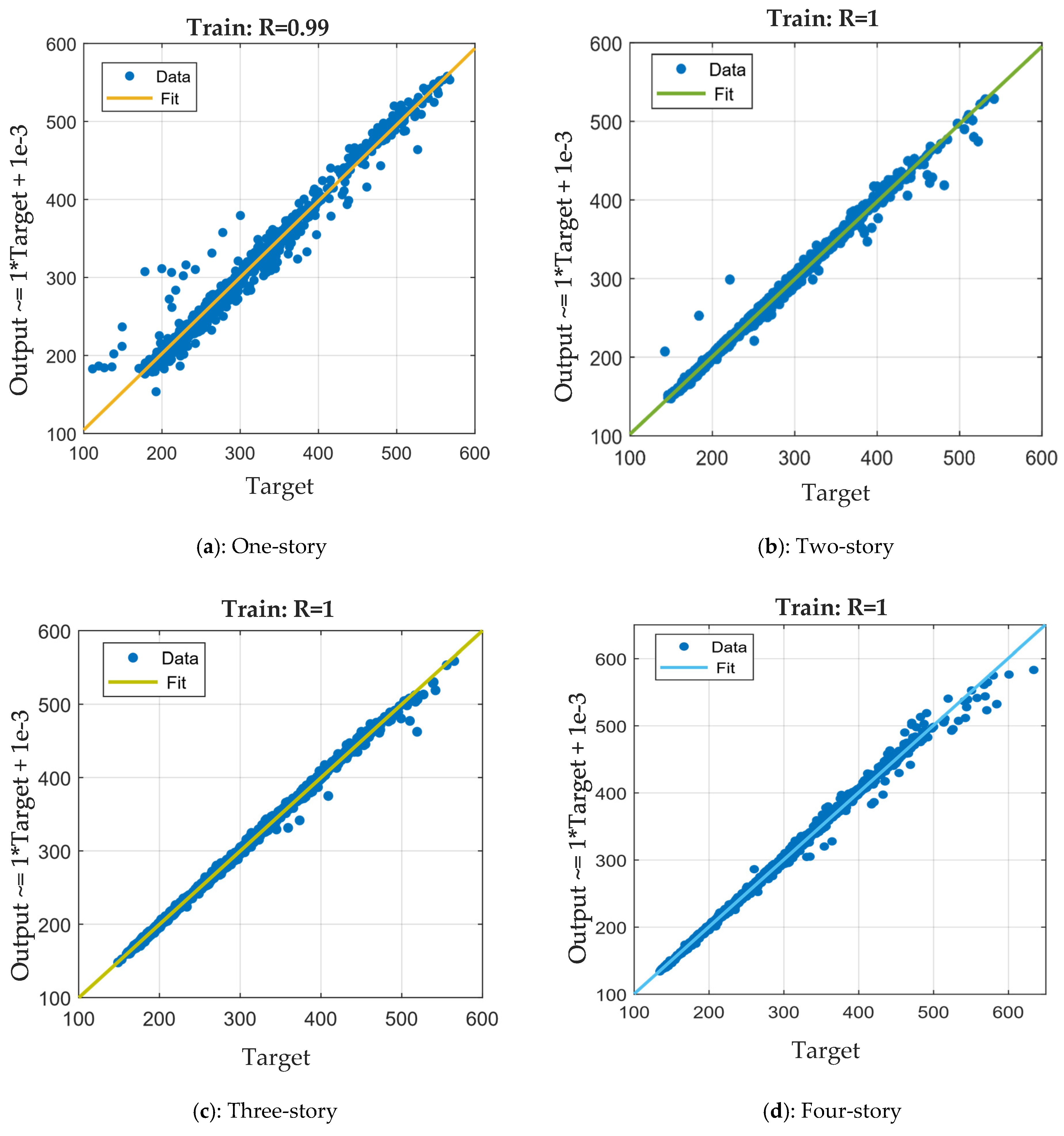
3.1. ANN Model Implementation and Evaluation
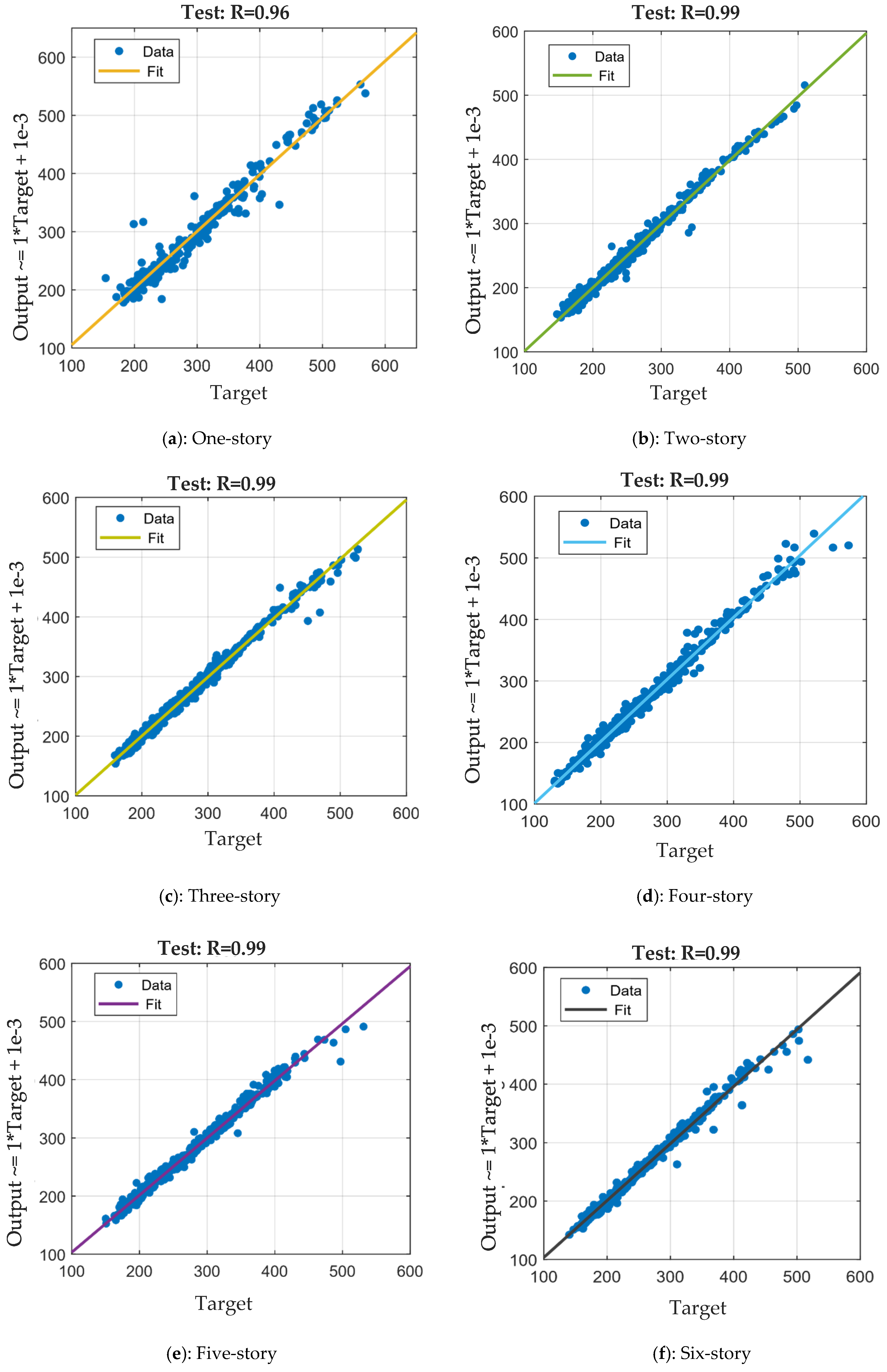
3.2. ANN Model Test
4. Discussion
5. Conclusions
Author Contributions
Funding
Data Availability Statement
Conflicts of Interest
Appendix A

| Split | MSE | MAE | R2 |
|---|---|---|---|
| 1 | 939.0496 | 21.83702 | 0.89035 |
| 2 | 749.8182 | 20.5306 | 0.988976 |
| 3 | 780.7594 | 20.31307 | 0.966402 |
| 4 | 1446.016 | 31.32112 | 0.845466 |
| 5 | 805.7235 | 19.8444 | 0.958779 |
| 6 | 822.5077 | 20.58016 | 0.911912 |
| 7 | 713.2101 | 22.20475 | 0.922691 |
| 8 | 1116.828 | 25.47749 | 0.875345 |
| 9 | 1314.102 | 27.45257 | 0.846268 |
| 10 | 1287.837 | 28.80976 | 0.868285 |
| Split | MSE | MAE | R2 |
|---|---|---|---|
| 1 | 464.0963 | 16.97236 | 0.956078 |
| 2 | 319.1598 | 14.42472 | 0.972284 |
| 3 | 236.7575 | 11.54886 | 0.953113 |
| 4 | 301.3321 | 14.23381 | 0.98236 |
| 5 | 608.8213 | 19.05794 | 0.894096 |
| 6 | 504.7459 | 16.83704 | 0.895332 |
| 7 | 473.9696 | 16.35537 | 0.91134 |
| 8 | 373.1442 | 15.27167 | 0.922211 |
| 9 | 156.7906 | 8.756949 | 0.972593 |
| 10 | 2987.873 | 39.91669 | 0.354073 |
| Split | MSE | MAE | R2 |
|---|---|---|---|
| 1 | 646.2045 | 19.35852 | 0.896962 |
| 2 | 436.3593 | 15.67782 | 0.959128 |
| 3 | 531.051 | 17.39965 | 0.914568 |
| 4 | 566.1927 | 18.10551 | 0.909988 |
| 5 | 307.6571 | 12.73632 | 0.948646 |
| 6 | 666.7583 | 19.57476 | 0.956311 |
| 7 | 545.1042 | 16.77145 | 0.967526 |
| 8 | 854.5338 | 22.51095 | 0.868376 |
| 9 | 702.5794 | 20.27778 | 0.88566 |
| 10 | 7533.805 | 62.61027 | −0.31858 |
| Split | MSE | MAE | R2 |
|---|---|---|---|
| 1 | 514.1374 | 17.71264 | 0.934243 |
| 2 | 628.5542 | 20.27511 | 0.914637 |
| 3 | 635.4107 | 19.24143 | 0.914544 |
| 4 | 821.0995 | 22.36189 | 0.92523 |
| 5 | 343.3422 | 13.97604 | 0.944394 |
| 6 | 934.4415 | 22.9563 | 0.898685 |
| 7 | 955.4811 | 26.99375 | 0.882358 |
| 8 | 932.7975 | 23.17373 | 0.873017 |
| 9 | 507.6461 | 17.30549 | 0.95854 |
| 10 | 1257.501 | 26.80686 | 0.823442 |
| Split | MSE | MAE | R2 |
|---|---|---|---|
| 1 | 774.728 | 22.9731 | 0.85631 |
| 2 | 605.2751 | 19.20743 | 0.8887 |
| 3 | 1012.153 | 26.10465 | 0.812985 |
| 4 | 768.4396 | 21.19448 | 0.854475 |
| 5 | 779.7878 | 22.04807 | 0.863658 |
| 6 | 747.039 | 21.14102 | 0.854186 |
| 7 | 1533.62 | 32.39531 | 0.810655 |
| 8 | 861.8436 | 23.67999 | 0.840125 |
| 9 | 915.7927 | 23.8359 | 0.843062 |
| 10 | 833.6425 | 21.51158 | 0.835395 |
| Split | MSE | MAE | R2 |
|---|---|---|---|
| 1 | 2465.79 | 40.18608 | 0.617101 |
| 2 | 842.8247 | 21.4921 | 0.889756 |
| 3 | 1051.855 | 24.80063 | 0.878674 |
| 4 | 758.6346 | 19.97696 | 0.899484 |
| 5 | 811.8736 | 21.84069 | 0.958785 |
| 6 | 674.8115 | 18.66438 | 0.861743 |
| 7 | 553.5335 | 18.42321 | 0.966595 |
| 8 | 747.5098 | 19.84545 | 0.873888 |
| 9 | 1031.597 | 23.45245 | 0.957008 |
| 10 | 642.9714 | 18.37619 | 0.866949 |
References
- Berardi, U. A cross-country comparison of the building energy consumptions and their trends. Resour. Conserv. Recycl. 2017, 123, 230–241. [Google Scholar] [CrossRef]
- Gaglia, A.G.; Dialynas, E.N.; Argiriou, A.A.; Kostopoulou, E.; Tsiamitros, D.; Stimoniaris, D.; Laskos, K.M. Energy performance of European residential buildings: Energy use, technical and environmental characteristics of the Greek residential sector–energy conservation and CO2 reduction. Energy Build. 2019, 183, 86–104. [Google Scholar] [CrossRef]
- Harvey, L.D.; Korytarova, K.; Lucon, O.; Roshchanka, V. Construction of a global disaggregated dataset of building energy use and floor area in 2010. Energy Build. 2014, 76, 488–496. [Google Scholar] [CrossRef]
- Yoshino, H.; Hong, T.; Nord, N. IEA EBC annex 53: Total energy use in buildings—Analysis and evaluation methods. Energy Build. 2017, 152, 124–136. [Google Scholar] [CrossRef]
- Wang, Z.; Srinivasan, R.S. A review of artificial intelligence based building energy use prediction: Contrasting the capabilities of single and ensemble prediction models. Renew. Sustain. Energy Rev. 2017, 75, 796–808. [Google Scholar] [CrossRef]
- Nejat, P.; Jomehzadeh, F.; Taheri, M.M.; Gohari, M.; Majid, M.Z.A. A global review of energy consumption, CO2 emissions and policy in the residential sector (with an overview of the top ten CO2 emitting countries). Renew. Sustain. Energy Rev. 2015, 43, 843–862. [Google Scholar] [CrossRef]
- Pablo-Romero, M.d.P.; Pozo-Barajas, R.; Yñiguez, R. Global changes in residential energy consumption. Energy Policy 2017, 101, 342–352. [Google Scholar] [CrossRef]
- Amasyali, K.; El-Gohary, N.M. A review of data-driven building energy consumption prediction studies. Renew. Sustain. Energy Rev. 2018, 81, 1192–1205. [Google Scholar] [CrossRef]
- Kontokosta, C.E. Energy disclosure, market behavior, and the building data ecosystem. Ann. N. Y. Acad. Sci. 2013, 1295, 34–43. [Google Scholar] [CrossRef]
- Papadopoulos, S.; Kontokosta, C.E. Using city benchmarking data to grade buildings on energy performance. Appl. Energy 2019, 233, 244–253. [Google Scholar] [CrossRef]
- Ribeiro, D. Developments in local energy efficiency policy: A review of recent progress and research. Curr. Sustain./Renew. Energy Rep. 2018, 5, 109–115. [Google Scholar] [CrossRef]
- Gao, X.; Malkawi, A. A new methodology for building energy performance benchmarking: An approach based on intelligent clustering algorithm. Energy Build. 2014, 84, 607–616. [Google Scholar] [CrossRef]
- Hsu, D. Improving energy benchmarking with self-reported data. Build. Res. Inf. 2014, 42, 641–656. [Google Scholar] [CrossRef]
- Kontokosta, C.E. A market-specific methodology for a commercial building energy performance index. J. Real Estate Financ. Econ. 2015, 51, 288–316. [Google Scholar] [CrossRef]
- Scofield, J.H. Energy star building benchmarking scores: Good idea, bad science. In Proceedings of the ACEEE Summer Study on Energy Efficiency in Buildings, Pacific Grove, CA, USA, 17–22 August 2014; pp. 267–282. [Google Scholar]
- Wei, Y.; Zhang, X.; Shi, Y.; Xia, L.; Pan, S.; Wu, J.; Han, M.; Zhao, X. A review of data-driven approaches for predicting and classifying building energy consumption. Renew. Sustain. Energy Rev. 2018, 82, 1027–1047. [Google Scholar] [CrossRef]
- Benavente-Peces, C.; Ibadah, N. Buildings energy efficiency analysis and classification using various machine learning technique classifiers. Energies 2020, 13, 3497. [Google Scholar] [CrossRef]
- Habib, F.; Barzegar, Z.; Hasabani, M.G. Prioritization of Effective Building Energy Consumer Parameters by AHP Deployment. Naqshejahan 2014, 4, 47–53. [Google Scholar]
- Omrany, H.; Marsono, A. Optimization of Building Energy Performance through Passive Design Strategies. Br. J. Appl. Sci. Technol. 2016, 13, 1–16. [Google Scholar] [CrossRef]
- Manzan, M. Genetic optimization of external fixed shading devices. Energy Build. 2014, 72, 431–440. [Google Scholar] [CrossRef]
- Seyedzadeh, S.; Rahimian, F.P.; Glesk, I.; Roper, M. Machine learning for estimating building energy consumption and performance: A review. Vis. Eng. 2018, 6, 5. [Google Scholar] [CrossRef]
- Ahmadnejad, F.; Shahbazi, Y.; Mokhtari Keshavar, M.; Zendeh Laleh, M.; HosseinPour, S.; KhaliliKhoo, N. The Effect of Shader’s Type, Depth and Distance on Optimizing Daylight Autonomy in High Rise Buildings in Cold Climate. Int. J. Archit. Eng. Urban Plan. 2023, 33, 57–73. [Google Scholar] [CrossRef]
- Ghaffari, A.; Shahbazi, Y.; Mokhtari Kashavar, M.; Fotouhi, M.; Pedrammehr, S. Advanced Predictive Structural Health Monitoring in High-Rise Buildings Using Recurrent Neural Networks. Buildings 2024, 14, 3261. [Google Scholar] [CrossRef]
- Shahbazi, Y.; Abdkarimi, M.; Ahmadnejad, F.; Mokhtari Kashavar, M.; Fotouhi, M.; Pedrammehr, S. Comparative Study of Optimal Flat Double-Layer Space Structures with Diverse Geometries through Genetic Algorithm. Buildings 2024, 14, 2816. [Google Scholar] [CrossRef]
- Shahbazi, Y.; Ghofrani, M.; Pedrammehr, S. Aesthetic Assessment of Free-Form Space Structures Using Machine Learning Based on the Expert’s Experiences. Buildings 2023, 13, 2508. [Google Scholar] [CrossRef]
- Singaravel, S.; Suykens, J.; Geyer, P. Deep-learning neural-network architectures and methods: Using component-based models in building-design energy prediction. Adv. Eng. Inform. 2018, 38, 81–90. [Google Scholar] [CrossRef]
- Chou, J.-S.; Tran, D.-S. Forecasting energy consumption time series using machine learning techniques based on usage patterns of residential householders. Energy 2018, 165, 709–726. [Google Scholar] [CrossRef]
- Wei, N.; Li, C.; Peng, X.; Zeng, F.; Lu, X. Conventional and artificial intelligence-based models for energy consumption forecasting: A review. J. Pet. Sci. Eng. 2019, 181, 106187. [Google Scholar] [CrossRef]
- Runge, J.; Zmeureanu, R. Forecasting energy use in buildings using artificial neural networks: A review. Energies 2019, 12, 3254. [Google Scholar] [CrossRef]
- Nie, P.; Roccotelli, M.; Fanti, M.P.; Ming, Z.; Li, Z. Prediction of home energy consumption based on gradient boosting regression tree. Energy Rep. 2021, 7, 1246–1255. [Google Scholar] [CrossRef]
- Khalil, M.; McGough, A.S.; Pourmirza, Z.; Pazhoohesh, M.; Walker, S. Machine Learning, Deep Learning and Statistical Analysis for forecasting building energy consumption—A systematic review. Eng. Appl. Artif. Intell. 2022, 115, 105287. [Google Scholar] [CrossRef]
- Olu-Ajayi, R.; Alaka, H.; Owolabi, H.; Akanbi, L.; Ganiyu, S. Data-driven tools for building energy consumption prediction: A review. Energies 2023, 16, 2574. [Google Scholar] [CrossRef]
- Liu, H.; Liang, J.; Liu, Y.; Wu, H. A review of data-driven building energy prediction. Buildings 2023, 13, 532. [Google Scholar] [CrossRef]
- Guyot, D.; Giraud, F.; Simon, F.; Corgier, D.; Marvillet, C.; Tremeac, B. Overview of using artificial neural networks for energy-related applications in the building sector. Int. J. Energy Res. 2019, 43, 6680–6720. [Google Scholar]
- Lu, C.; Li, S.; Lu, Z. Building energy prediction using artificial neural networks: A literature survey. Energy Build. 2022, 262, 111718. [Google Scholar] [CrossRef]
- Afzal, S.; Ziapour, B.M.; Shokri, A.; Shakibi, H.; Sobhani, B. Building energy consumption prediction using multilayer perceptron neural network-assisted models; comparison of different optimization algorithms. Energy 2023, 282, 128446. [Google Scholar] [CrossRef]
- Tsoka, T.; Ye, X.; Chen, Y.; Gong, D.; Xia, X. Explainable artificial intelligence for building energy performance certificate labelling classification. J. Clean. Prod. 2022, 355, 131626. [Google Scholar] [CrossRef]
- Elbeltagi, E.; Wefki, H. Predicting energy consumption for residential buildings using ANN through parametric modeling. Energy Rep. 2021, 7, 2534–2545. [Google Scholar] [CrossRef]
- Elbeltagi, E.; Wefki, H.; Abdrabou, S.M.; Dawood, M.; Ramzy, A. Visualized strategy for predicting buildings energy consumption during early design stage using parametric analysis. J. Build. Eng. 2017, 13, 127–136. [Google Scholar] [CrossRef]
- Boumaraf, H.; İnceoglu, M. Computational analysis for design development evaluation in spatial planning. Eskişehir Tech. Univ. J. Sci. Technol. A-Appl. Sci. Eng. 2022, 23, 94–111. [Google Scholar] [CrossRef]
- LadybugTools. LadybugTools LLC. Available online: https://www.ladybug.tools/ (accessed on 1 July 2024).
- Food4Rhino. Available online: https://www.food4rhino.com/en/app/octopus (accessed on 10 July 2024).
- da Silva, M.A.; Garcia, R.d.P.; Carlo, J.C. Multi-objective optimization algorithms for building performance assessment—A benchmark. Int. J. Archit. Comput. 2024, 14780771241296263. [Google Scholar] [CrossRef]
- Demšar, J.; Curk, T.; Erjavec, A.; Gorup, C.; Hočevar, T.; Milutinovič, M.; Možina, M.; Polajnar, M.; Toplak, M.; Starič, A.; et al. Orange: Data Mining Toolbox in Python. J. Mach. Learn. Res. 2013, 14, 2349–2353. [Google Scholar]
- Ren, Z.; Tang, Z.; James, M. Predictive Weather Files for Building Energy Modelling User Guide; CSIRO: Canberra, Australia, 2021. [Google Scholar]
- Energyplus Weather Data. Available online: https://www.energyplus.net/weather (accessed on 2 July 2024).
- Abraham, A. Handbook of Measuring System Design; Sydenham, P.H., Thorn, R., Eds.; John Wiley & Sons, Ltd.: Hoboken, NJ, USA, 2005; Available online: https://onlinelibrary.wiley.com/doi/epdf/10.1002/0471497398.mm421 (accessed on 2 July 2024).
- Zhang, G.; Patuwo, B.E.; Hu, M.Y. Forecasting with artificial neural networks: The state of the art. Int. J. Forecast. 1998, 14, 35–62. [Google Scholar] [CrossRef]
- Specht, D.F. A general regression neural network. IEEE Trans. Neural Netw. 1991, 2, 568–576. [Google Scholar] [CrossRef]
- Trzepieciński, T. The comparison of the multi-layer artificial neural network training methods in terms of the predictive quality of the coefficient of friction of 1.0338 (DC04) Steel Sheet. Materials 2024, 17, 908. [Google Scholar] [CrossRef]
- Kalinić, Z.; Marinković, V.; Kalinić, L.; Liébana-Cabanillas, F.J. Neural network modeling of consumer satisfaction in mobile commerce: An empirical analysis. Expert Syst. Appl. 2021, 175, 114803. [Google Scholar] [CrossRef]
- Altman, N.S. An Introduction to Kernel and Nearest-Neighbor Nonparametric Regression. Am. Stat. 1992, 46, 175–185. [Google Scholar] [CrossRef]
- ISIRI 14253; Residential Building—Criteria for Energy Consumption and Energy Labeling Instruction. Institute of Standards Islamic Republic of Iran: Tehran, Iran, 2011.


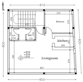
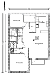
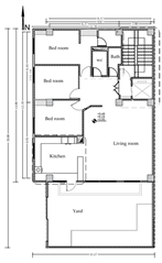
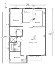
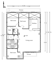
| Number of Floors | Plans (Scale 1:100) | 3D Models | ||
|---|---|---|---|---|
| 2 | Pilot | 1 st Floor | 2nd Floor | 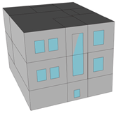 |
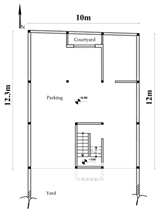 | 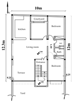 |  | ||
| 3 | 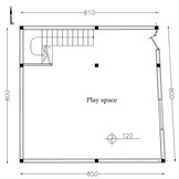 | 1st, 2nd, and 3rd Floors | 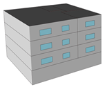 | |
 | ||||
| 4 | 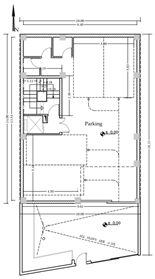 | 1st, 2nd, 3rd, and 4th Floors | 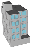 | |
 | ||||
| 5 |  | 1st to 3rd Floors | 4th and 5th Floors | 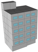 |
 |  | |||
| 6 | 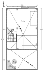 | 1st to 5th Floors | 6th Floor | 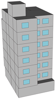 |
 |  | |||
| Variables | |
|---|---|
| Continuous | Discrete |
| Plan Area | Geometric Plan Points |
| Plan Perimeter | Plan Scale (Length and Width) |
| Volume | Orientation |
| VSR | Internal Wall Area |
| APR | - |
| WWR | - |
| Shader Depth | - |
| Sample Buildings | Actual Energy Consumption (kWh/year) | Annual Energy Consumption Extracted from the Parametric Model (kWh/year) | Difference (%) |
|---|---|---|---|
| One-story | 368.3268 | 381.4126 | 3.4 |
| Two-story | 307.5252 | 320.6377 | 4 |
| Three-story | 405.24 | 390.0091 | 3.9 |
| Four-story | 451.2668 | 430.7079 | 4.5 |
| Five-story | 342.93 | 360.67 | 4.9 |
| Six-story | 286.5476 | 294.1308 | 2.6 |
| Model Inputs | U | Model Output | U |
|---|---|---|---|
| Orientation | ° | Annual energy consumption | |
| Volume | m3 | ||
| AREA | m2 | ||
| Perimeter | m | ||
| APR | m | ||
| VSR | m | ||
| Int_Wall_Area | m2 | ||
| N_WWR | % | ||
| w_WWR | % | ||
| s_WWR | % | ||
| E_WWR | % | ||
| N_shader’s Depth | m | ||
| W_shader’s Depth | m | ||
| S_shader’s Depth | m | ||
| E_shader’s Depth | m |
| Row | Climate Type | City | Ideal Building Energy Consumption Index (kWh/m2/Year) | |
|---|---|---|---|---|
| Small Residential | Large Residential | |||
| 1 | Very cold | Sarab | 111 | 102 |
| 2 | Cold | Tabriz | ||
| 3 | Moderate and rainy | Rasht | 156 | 106 |
| 4 | Semi-arid | Moghan | ||
| 5 | Warm and dry | Tehran | 83 | 87 |
| 6 | Very hot and dry | Zahedan | 86 | 75 |
| 7 | Very hot and dry | Ahvaz | 150 | 138 |
| 8 | Very hot and humid | Bandar Abbas | 130 | 118 |
| Energy | Use | |
|---|---|---|
| Small Residential | Large Residential | |
| A | R < 1 | R < 1 |
| B | 1.0 < R < 2.0 | 1.0 < R < 1.9 |
| C | 2.0 < R < 2.9 | 1.9 < R < 2.7 |
| D | 2.9 < R < 3.7 | 2.7 < R < 3.4 |
| E | 3.7 < R < 4.0 | 3.4 < R < 4.0 |
| F | 4.4 < R < 5.0 | 4.0 < R < 4.5 |
| G | 5.0 < R < 5.4 | 4.5 < R < 5.0 |
| The label is not awarded | 5.4 ≤ R | 5.0 ≤ R |
| Number of Hidden Layers | Number of Neurons | Activation Functions | Optimizer | MSE | MAE | R2 |
|---|---|---|---|---|---|---|
| One | 30 | Re Lu | Adam | 0.006 | 0.059 | 0.835 |
| One | 40 | Re Lu | Adam | 0.007 | 0.071 | 0.781 |
| One | 50 | Re Lu | Adam | 0.005 | 0.056 | 0.851 |
| One | 60 | Re Lu | Adam | 0.005 | 0.057 | 0.853 |
| One | 70 | Re Lu | Adam | 0.003 | 0.043 | 0.893 |
| One | 80 | Re Lu | Adam | 0.004 | 0.041 | 0.894 |
| One | 90 | Re Lu | Adam | 0.004 | 0.050 | 0.876 |
| Two | 70, 70 | Re Lu | Adam | 0.002 | 0.037 | 0.920 |
| Two | 80, 80 | Re Lu | Adam | 0.002 | 0.037 | 0.944 |
| Two | 90, 90 | Re Lu | Adam | 0.002 | 0.031 | 0.932 |
| Two | 100, 100 | Re Lu | Adam | 0.002 | 0.031 | 0.950 |
| Two | 150, 150 | Re Lu | Adam | 0.002 | 0.030 | 0.941 |
| Two | 200, 200 | Re Lu | Adam | 0.001 | 0.021 | 0.951 |
| Three | 30, 30, 30 | Re Lu | Adam | 0.004 | 0.040 | 0.880 |
| Three | 40, 40, 40 | Re Lu | Adam | 0.002 | 0.030 | 0.922 |
| Three | 50, 50, 50 | Re Lu | Adam | 0.003 | 0.031 | 0.922 |
| Number of Hidden Layers | Number of Neurons | Activation Functions | Optimizer | MSE | MAE | R2 |
|---|---|---|---|---|---|---|
| Two | 100, 50 | Re Lu | Adam | 0.002 | 0.030 | 0.912 |
| Two | 100, 60 | Re Lu | Adam | 0.001 | 0.021 | 0.940 |
| Two | 100, 70 | Re Lu | Adam | 0.002 | 0.031 | 0.931 |
| Two | 100, 80 | Re Lu | Adam | 0.002 | 0.030 | 0.934 |
| Two | 100, 90 | Re Lu | Adam | 0.001 | 0.021 | 0.951 |
| Two | 90, 80 | Re Lu | Adam | 0.001 | 0.022 | 0.939 |
| Two | 100, 70 | Re Lu | Adam | 0.001 | 0.021 | 0.952 |
| Two | 250, 160 | Re Lu | Adam | 0.001 | 0.022 | 0.965 |
| Two | 120, 200 | Re Lu | Adam | 0.001 | 0.023 | 0.954 |
| Two | 80, 110 | Re Lu | Adam | 0.002 | 0.031 | 0.922 |
| Two | 80, 240 | Re Lu | Adam | 0.002 | 0.030 | 0.924 |
| Number of Hidden Layers | Number of Neurons | Activation Functions | Optimizer | MSE | MAE | R2 |
|---|---|---|---|---|---|---|
| Two | 100, 90 | Identify | Adam | 0.001 | 0.031 | 0.931 |
| Two | 100, 90 | Hyperbolic | Adam | 0.001 | 0.019 | 0.948 |
| Two | 100, 90 | Re Lu | LB | 0.002 | 0.022 | 0.958 |
| Two | 100, 90 | Hyperbolic | SGD | 0.080 | 0.034 | 0.718 |
| Two | 100, 90 | Identify | SGD | 0.030 | 0.014 | 0.722 |
| Two | 250, 160 | Re Lu | Adam | 0.001 | 0.022 | 0.965 |
| Two | 250, 160 | Hyperbolic | SGD | 0.009 | 0.011 | −0.011 |
| Two | 250, 160 | Hyperbolic | Adam | 0.030 | 0.041 | 0.891 |
| Two | 120, 200 | Logistic | LB | 0.000 | 0.497 | 0.989 |
| Two | 120, 200 | Re Lu | LB | 0.000 | 0.504 | 0.981 |
| Two | 120, 200 | Identify | SGD | 0.030 | 0.071 | −0.012 |
| Parameters | U | Simulation Data Sample | |||||
|---|---|---|---|---|---|---|---|
| 1 F-Bldng | 2 F-Bldng | 3 F-Bldng | 4 F-Bldng | 5 F-Bldng | 6 F-Bldng | ||
| Orientation | 255 153.1253 | 120 | 105 | 345 | 15 | 0 | |
| Volume | 153.1253 | 1756.14 | 2526.075 263.1328 | 3203.862 250.3017 | 4709.286 | 5441.415 | |
| AREA | 42.5348 | 274.3969 | 263.1328 | 250.3017 | 294.3304 131.8798 | 283.407 | |
| Perimeter | 42.424 | 102.8258 | 114.2494 | 115.6026 | 131.8798 131.8798 | 109.5606 | |
| APR | 1.002612 | 2.668561 | 2.303144 3.860198 | 2.165191 | 2.231808 | 2.58676 | |
| VSR | 2.886528 120 120 | 5.739397 | 3.860198 | 5.05233 | 7.043378 | 3.68263 | |
| Int_Wall_Area | 120 | 323 0.66 0.66 | 237 | 43 | 47 | 177 | |
| N_WWR | % | 0.94 0.92 0.92 | 0.66 | 0.85 | 0.19 0.89 | 0.37 | 0 |
| W_WWR | % | 0.92 | 0.45 | 0.11 | 0.89 | 0.91 | 0.81 |
| S_WWR | % | 0.7 | 0.26 | 0.1 | 0.86 | 0.79 | 0.08 |
| E_WWR | % | 0.09 | 0.74 | 0.59 | 0.35 | 0.89 | 0.61 |
| N_shader’s Depth | 0.7 | 1.2 | 0.4 | 0.2 | 0.2 | 1.1 | |
| W_shader’s Depth | 1.3 | 1.1 | 0.4 | 0.5 | 1.1 | 1.4 | |
| S_shader’s Depth | 0 | 0.9 | 0.2 | 0.8 | 0.1 | 0.8 | |
| E_shader’s Depth | 0.4 | 0.2 | 1.1 | 1.5 | 0.6 | 0 | |
| Total Energy | 500.5713 | 175.5731 | 200.3133 | 208.0642 | 201.7758 | 166.5841 | |
| Predicted Energy consumption | 506.175 | 172.505 | 199.343 | 207.739 | 205.817 | 165.05 | |
| Energy consumption Grade | G | B | B | C | C | B | |
Disclaimer/Publisher’s Note: The statements, opinions and data contained in all publications are solely those of the individual author(s) and contributor(s) and not of MDPI and/or the editor(s). MDPI and/or the editor(s) disclaim responsibility for any injury to people or property resulting from any ideas, methods, instructions or products referred to in the content. |
© 2025 by the authors. Licensee MDPI, Basel, Switzerland. This article is an open access article distributed under the terms and conditions of the Creative Commons Attribution (CC BY) license (https://creativecommons.org/licenses/by/4.0/).
Share and Cite
Shahbazi, Y.; Hosseinpour, S.; Mokhtari Kashavar, M.; Fotouhi, M.; Pedrammehr, S. Developing an Artificial Neural Network-Based Grading Model for Energy Consumption in Residential Buildings. Buildings 2025, 15, 1731. https://doi.org/10.3390/buildings15101731
Shahbazi Y, Hosseinpour S, Mokhtari Kashavar M, Fotouhi M, Pedrammehr S. Developing an Artificial Neural Network-Based Grading Model for Energy Consumption in Residential Buildings. Buildings. 2025; 15(10):1731. https://doi.org/10.3390/buildings15101731
Chicago/Turabian StyleShahbazi, Yaser, Sahar Hosseinpour, Mohsen Mokhtari Kashavar, Mohammad Fotouhi, and Siamak Pedrammehr. 2025. "Developing an Artificial Neural Network-Based Grading Model for Energy Consumption in Residential Buildings" Buildings 15, no. 10: 1731. https://doi.org/10.3390/buildings15101731
APA StyleShahbazi, Y., Hosseinpour, S., Mokhtari Kashavar, M., Fotouhi, M., & Pedrammehr, S. (2025). Developing an Artificial Neural Network-Based Grading Model for Energy Consumption in Residential Buildings. Buildings, 15(10), 1731. https://doi.org/10.3390/buildings15101731