Abstract
The persistent carbon lock-in in transport infrastructure hinders low-carbon transition and sustainable urban development. This study, situated within the context of building energy and systems environments, examines the spatial and temporal dynamics of carbon lock-in across Chinese provinces over the past decade. A composite indicator system is constructed to quantify path dependence in transport-related carbon emissions. Additionally, a quantile regression model is applied to analyze the heterogeneous effects of influencing factors across varying levels of lock-in. The findings offer insights into developing region-specific decarbonization strategies and enhancing the sustainability of infrastructure systems. The key findings are as follows: (1) temporally, the composite path dependence index (PDI) increased from 0.13 to 0.24, with an average annual growth rate of 5.7%, although the growth trend exhibited noticeable fluctuations. (2) Spatially, a clear “East-High–West-Low, South-High–North-Low” pattern is observed, with the eastern region exhibiting a PDI approximately 29% higher than that of the northeastern region—mainly due to differences in economic vitality and the degree of policy intervention. (3) Threshold nonlinearity is evident: the influence of key factors on carbon path dependence varies across quantiles, and a critical threshold appears at the 0.9 quantile. Notably, the mitigating effect of low-carbon technological innovation on path dependence weakens beyond this threshold, suggesting diminishing marginal returns and the necessity for complementary governance strategies. This study deepens the understanding of transport carbon lock-in and provides guidance for region-specific strategies to enhance energy efficiency and sustainability in integrated building infrastructure systems.
1. Introduction
As environmental problems become increasingly severe, carbon emissions have become the primary focus of countries around the world. President Xi Jinping pointed out and emphasized that “Achieving carbon peak and carbon neutrality is a broad and profound economic and social systematic change, and carbon peak and car-bon neutrality should be integrated into the overall layout of the construction of eco-logical civilization”.
The proposal of the “dual-carbon” goal provides a directional guide and fundamental guideline for China’s economic and social transformation and development in a green and low-carbon manner. China’s carbon emissions are predominantly concentrated in three key sectors: industry, transportation, and construction. Among these, transportation serves as a foundational, pioneering, and strategic industry, as well as a critical service sector within the national economy. Current data indicates that CO2 emissions from China’s transportation sector account for approximately 10% of the nation’s total carbon emissions [1]. Globally, the transportation sector’s contribution to carbon emissions is even more significant. According to the International Energy Agency’s (IEA) latest Global Energy and CO2 Status Report, transportation-related emissions represent about 27% of total global carbon emissions [2], positioning it as a key focus area for carbon mitigation. In alignment with these challenges, China’s Outline of the National Comprehensive Three-dimensional Transportation Network Plan explicitly mandates accelerated green and low-carbon development, urging the transportation sector to achieve peak CO2 emissions as early as possible [3]. However, due to the huge demand of the transportation industry, the carbon emissions from transportation have still been growing in the past ten years. Transportation infrastructure construction has a large input of materials and energy consumption and a wide range of ecological disturbance, which is an important area for green and low-carbon transformation of the transportation industry [4]. Currently, the total amount of transportation infrastructure construction in China has jumped to the forefront of the world, but there are still problems of high-carbon emission intensity and insufficient coordinated development with the ecological environment. According to the life cycle assessment (LCA) study, the carbon emissions of its construction phase can account for more than 40% of the whole life cycle, and the continuous energy consumption in the operation and maintenance phase constitutes a long-term carbon source [5]. Accelerate the construction of green and low-carbon transportation infrastructure construction system, the concept of green and low-carbon throughout the entire process of transportation infrastructure planning, construction, operation and maintenance, accelerate the transformation and upgrading of production methods, has become a transportation infrastructure to implement the strategy of ecological civilization, the inevitable requirements of the service “dual-carbon” goal, but also to support the acceleration of the construction of a strong transportation country, It is also a key initiative to support the accelerated construction of a strong transportation country and promote the sustainable development of transportation [6].
Carbon lock-in, as an important challenge to the global energy system, imposes a serious load on the environmental system and is the biggest obstacle to the low-carbon transition. Carbon lock-in in transportation infrastructure describes a systemic phenomenon where long-lived, carbon-intensive infrastructure (e.g., highway networks, fuel supply systems, and aviation hubs) interacts with entrenched technological systems, institutional frameworks, and high-carbon economic models. This interaction fosters persistent reliance on fossil fuel technologies within transportation systems. As mature high-carbon technologies dominate markets through established advantages such as economies of scale, their associated industrial chains and infrastructure networks evolve into self-reinforcing closed-loop systems, further entrenching carbon-intensive pathways. When high-carbon technologies dominate the market by virtue of their maturity and economies of scale, their supporting industrial chains and infrastructure networks gradually form a self-reinforcing closed-loop system. This process is called “path dependence” [7,8]. The formation of carbon lock-in transportation infrastructure is the result of multiple factors. Firstly, the technological lock-in stems from the network effect and economies of scale of the established technology system, which is continuously strengthened through the synergistic effect of the upstream and downstream industrial chain [9]. Secondly, the lock-in at the institutional level is manifested in the path dependence of the policy framework, and the existing investment decision-making mechanism and performance evaluation system tend to maintain the status quo. However, carbon lock-in is not an unbreakable absolute state; with the advancement of low-carbon technology and institutional innovation, the lock-in intensity presents dynamic change characteristics. Studies have shown that the application of digital technology and the construction of new infrastructure provide an important opportunity for unlocking [10]. However, realizing carbon unlocking of transportation infrastructure requires overcoming multiple barriers such as technology conversion costs, institutional friction resistance, and social adaptation costs and adopting a systematic transformation strategy, including concerted efforts in multiple dimensions such as technological innovation, institutional restructuring, and market mechanism construction.
At present, with the proposal of a low-carbon transition development strategy, the research on carbon locking has achieved relatively rich results. Hong Jingke (2022) used the carbon emissions of buildings to measure the degree of carbon locking in the construction industry [11]. Niu Honglei (2021) constructed the measurement index system of the carbon locking effect from the four dimensions of fixed inputs, technology, institutions, and social behavior and pointed out that there is a degree of carbon locking in the east and west of China, and the overall locking, technology locking, and institutional locking show a decreasing trend [12,13]. differentiation, and the overall locking, technological locking, and institutional locking show a decreasing trend, and subsequently, the degree of carbon locking in the manufacturing industry is measured through the four dimensions of fixed inputs, technology, institutions, and market demand structure, and its spatio-temporal evolution characteristics. Liu Minghao (2023) used the efficiency measurement model—DEA—to measure the degree of carbon locking in the electric power industry in order to avoid the subjectivity of the locking degree measurement model [14]. Cai Haiya (2018) takes China’s industrial sector as the research object, measures China’s carbon lock-in situation with the help of the input-output model, explores the characteristics of the temporal and spatial differences in the carbon lock-in situation of the sub-industry industrial sector, and puts forward relevant countermeasures and suggestions based on the results of the study [15]. Tao et al. (2025) demonstrated that network infrastructure construction can break traditional economic inertia by stimulating green innovation and reducing energy market segmentation, though institutional lock-in remains persistent, providing empirical evidence of policy-driven carbon unlocking mechanisms [16]. Existing research on carbon lock-in primarily addresses macro-level societal, industrial, and regional perspectives, with a strong focus on energy and power sectors. However, studies targeting transportation infrastructure remain limited. For instance, Chen (2023) pioneered an evaluation framework analyzing the coupling coordination between technological, economic, and institutional systems in transportation carbon lock-in. Their findings reveal significant spatial heterogeneity in the carbon locking intensity of transportation infrastructure [10]. Shao (2025) analyzed the carbon lock-in effect of transportation infrastructure from the perspective of system coordination effect and interaction correspondence based on city-level panel data in Shandong Province [17].
To address the identified research gaps, this study aims to systematically investigate the path dependence mechanism of carbon lock-in in China’s provincial transportation infrastructure and propose spatially differentiated decarbonization strategies through an integrated methodological approach. Specifically, we pursue three objectives:
(1) To develop a multidimensional measurement framework integrating technological, economic, and institutional dimensions, operationalized by constructing a composite index system adapted from Chen’s framework [10] and enhanced with Pearson correlation analysis to quantify structural element interactions.
(2) To identify threshold characteristics and heterogeneous impacts of key drivers across infrastructure development stages, achieved through pioneering application of quantile panel regression models to 31 provinces’ panel data (2010–2022), which capture nonlinear effects obscured by conventional methods [18].
(3) To generate province-specific policy pathways for carbon unlocking, enabled by synthesizing spatial heterogeneity patterns from both the composite index and regression elasticity differentials.
2. Materials and Methods
2.1. Construction of Carbon Locked Path Dependence Indicator System for Transportation Infrastructure
In the process of indicator selection, based on the influencing factors of carbon locked path dependence of transportation infrastructure identified above, we first conducted Delphi expert consultation (9 practitioners) and grounded theory analysis to establish preliminary criteria. The indicators were subsequently screened and quantified through iterative refinement, strictly adhering to the quintuple principles of quantifiability, validity, representativeness, operability, and accessibility.
2.1.1. Technical Level Path Dependence Measurement Indicator
The quantitative indicators of the path-dependence effect of carbon lock-in of transportation infrastructure should reflect both inertia to traditional technology and insufficient low-carbon technological innovation in order to accurately reflect the level of technological path-dependence. As systematically presented in Table 1, this study chooses traditional technology inertia, low-carbon technology innovation, and low-carbon technology transformation cost as the first-level indicators for path dependence measurement.

Table 1.
Transportation infrastructure carbon lock-in technical path dependence measurement index system.
2.1.2. Economic Level Path Dependence Measurement Indicator
Regarding the path dependence of the carbon lock-in economic level of transportation infrastructure, this study first holds from the perspective of sunk cost that transportation infrastructure projects themselves have characteristics such as large investment and long life cycle. Sunk cost is an important reason for the path dependence of carbon lock-in in transportation infrastructure, as shown in Table 2. Once a project is put into use, it will generate a continuous high-carbon emission state that is difficult to change, which creates the initial conditions for the formation of path dependence.
Table 2.
Transportation infrastructure carbon lock-in economic path dependence measurement index system.
2.1.3. Regime-Level Path Dependence Measurement Indicator
Institutional embeddedness and the role of government are important conditions for the formation of institutional path dependence. Institutional embeddedness includes both high-carbon institutional rigidity and low-carbon institutional lag, and this paper chooses the degree of government intervention, high-carbon institutional rigidity, and low-carbon institutional lag to measure the intensity of path dependence at the institutional level of carbon lock-in for transportation infrastructure, as shown in Table 3.
Table 3.
Transportation infrastructure carbon lock-in regime path dependence measurement index system.
2.2. Transportation Infrastructure Carbon Locked Path Dependency Measurement Modeling
2.2.1. Measurement of the Path Dependence Index
First of all, this paper draws on the research of [11,19], using the entropy weight method to measure the weight of indicators. This method can be calculated according to the degree of difference between the indicators of the weight of the indicators, which can effectively overcome the errors brought about by subjectivity and can provide an objective basis for the comprehensive evaluation of multiple indicators. Considering that there are differences in the unit of measurement and order of magnitude in the data at the indicator level, referring to the study of [20], we choose to improve the method of standardization of extreme deviation to deal with the raw data and make the result 0~1 while eliminating the influence of the unit of magnitude. On this basis, we measure the comprehensive index of path dependence as well as the index of path dependence of the three sub-systems of economy, technology, and system, and the specific formulae are shown in (1).
where is the path dependence composite index of province i in year , is the composite weight of the indicator, and is the standardized value of indicator j in year of province i.
2.2.2. Pearson Correlation Coefficient
Referring to Mi Zefeng (2018) [19] and Li Da (2020) [21], the degree of fit between the numerical series of two similar periods in the model was determined by the Pearson correlation coefficient, and the existence of path dependence was screened by determining the degree of path correlation between the two periods. In this study, according to the evaluation index system of carbon locking path dependence of transport infrastructure, the structural similarity of different regions at different stages in different years is measured for the three systemic levels of technology, economy, and system, as well as the indicator level, in order to determine the degree of structural path dependence, and the specific formula is shown in (2).
where denotes the correlation coefficient of a province or region k at time (stage) x and time (stage) y; xi denotes the value of indicator i of a province or region k at time (stage) x; yi denotes the value of indicator i of a province or region k at time (stage) y, and n denotes the number of indicators. n = 9 when measuring correlation coefficients of a province or region as a whole, and n = 3 when measuring the technical, economic, and institutional system-level correlation coefficients when n = 3.
2.3. Dynamic Evolution of Path Dependence of Carbon Locking in Transport Infrastructure
2.3.1. Kernel Density Estimation Method
The kernel density estimation method is a non-parametric method used to monitor the evolutionary characteristics of data, which can measure the spatial distribution state, location, and evolutionary trends through continuous density curves, and the translation of the curves can show the overall trend of the data, and the width of the curves and changes in the shape of the peaks reveal the changes in the differences between the data. More general parameter estimation methods are parametric methods; there is no requirement for the data distribution, no need to assume that the data follow a specific distribution model [20,22]. Therefore, this paper combines the features of the kernel density estimation method and adopts the kernel density estimation curve to visualize the distribution pattern of the evolutionary trend of the carbon locking path dependence of China’s provincial transport infrastructures. The kernel density estimation function formula is as follows:
where f(x) is the estimated probability density function of path dependence at Xi, x represents the mean value of the degree of path dependence, Xi is the value of independent and identically distributed variables, K(x) is the kernel function representing the path dependence influences on carbon locking of transport infrastructure in each province, N is the total number of samples, and h is the bandwidth. In kernel density estimation methods, the choice of kernel function has diversity, and common types include uniform kernel, triangular kernel, and Gaussian kernel. It has been shown that despite the differences in the mathematical forms of different kernel functions, their effects on the estimation results are usually in a controllable range and relatively limited. In view of this, this study employs a Gaussian kernel (GK) function to estimate the distribution density of the path-dependent effects of carbon locking in transport infrastructure in different regions to capture its spatial heterogeneity characteristics. The method can effectively portray the distribution pattern of variables in the sample space through the construction of a continuous probability density function. The specific expressions are shown below:
A shift of the curve to the right indicates an increase in the overall value of the data; conversely, it indicates a decrease; a broad curve indicates a large shape difference, while a narrow curve implies a smaller difference. Multiple peaks may indicate the presence of several different groups in the data. In addition, the length of the tail of the curve shows us the degree of extreme variation in the distribution of the data; the longer the tail, the more extreme values in the data.
2.3.2. Dagum’s Gini Coefficient Method and Its Decomposition
The Dagum Gini coefficient was proposed by Dagum in 1997 on the basis of the traditional Gini coefficient, which is commonly used to analyze regional spatial variability. This method not only makes up for the defects of small sample size, heteroskedasticity, and asymmetry of distribution of the Tyrell index, but also effectively analyzes the source of spatial disparity [23,24]. In this paper, the Gini coefficient method and its decomposition method are used to analyze the spatial heterogeneity of carbon locked path dependence of transport infrastructure, and the basic formula of the Gini coefficient is shown below:
where k denotes the four regions of east, northeast, central, and west; l and r denote the serial numbers of the provinces within the region; nj and nh denote the number of provinces within the region of j and h, respectively; denotes the mean value of carbon locked path dependence of transport infrastructure; and the total number of samples is , the Dagum’s Gini coefficient can decompose the inequality of the whole into the following three parts: intra-group variance Gw reflects the uneven distribution of path dependence distribution; inter-group inequality Gb indicates the uneven distribution of path dependence between different regions; hypervariance density Gt reacts to the uneven distribution of path dependence in the overlapping part between different regions, and its calculation formula is as follows:
where Gjj is the Gini coefficient within region j; Gjh is the Gini coefficient between region j and region h, and and denote the average of the carbon locked path dependence of transport infrastructure for the provinces included in region j and region h, respectively.
2.4. Panel Quantile Regression Model
Koenker first initiated the exploration of quantile regression models for panel data by applying quantile regression to longitudinal data analysis and proposing fixed effects longitudinal data quantile regression, which is an important extension of the measurement methodology for panel data, which is characterized by a large sample size, the ability to incorporate both cross-sectional and temporal dimensions, and the ability to address the problem of omitted variables [25]. The quantile regression method, with its ability to portray the multidimensional characteristics of the data distribution, is an important complement to the traditional mean regression model. Compared with the ordinary least squares (OLS) method based on the conditional mean assumption, quantile regression can effectively control individual heterogeneity, make full use of the advantages of the large sample of panel data, and is especially suitable for dealing with non-normally distributed data with spatial and temporal heterogeneity, which often show the characteristics of high peaks, heteroskedasticity, and significant deviation from normal distribution, and OLS estimation is easy to ignore the information in the tails of the distribution, which leads to biased results. Results. Panel quantile regression, through the differential estimation of the effect of the explanatory variables at different quantiles of the explanatory variables, is able to capture the response characteristics of the variables in the full distribution, avoiding the simplified treatment of the overall characteristics of the data by mean regression, and thus providing more robust and comprehensive estimation results under the scenarios of heterogeneous shocks or coefficient fluctuations. Therefore, in this paper, the panel quantile regression model is chosen to analyze the influencing factors of carbon locked path dependence of transport infrastructure. Differential estimates of the impact effects of each influencing factor at different points of the path dependence can be obtained.
A panel data model is assumed to be available:
where x is the k × 1 dimensional vector of explanatory variables for the ith individual cross-section in period t; β is the k × 1 dimensional vector of coefficients; a is the ith individual effect and is the intercept term for individual heterogeneity; if a is related to one of the explanatory variables, then it is called an individual fixed effects model: if a is not related to all of the explanatory variables, then it is called an individual random-effects model. Assuming α is the cross-sectional solid effect, which represents unobservable factors that are not accounted for in the regression model but are closely related to individual variation. At any quantile r, a conditional quantile function corresponding to the observed values can be established:
where α(t) and β(t) are the parameters to be estimated. If the number of observations is sufficiently large, it is possible to estimate the fixed effect α(t) for each individual at quartile t. However, when the number of individual cross-sections is large, the number of α(t) to be estimated can be very large. To reduce the number of parameters to be estimated, we assume that the value of the individual fixed effect α does not depend on the quantile τ and only consider the effect of the independent variable x on the dependent variable, i.e., the coefficient β(t) that varies with the quantile. Equations (12)–(15) are modified to a conditional quantile function as follows:
Finally, it combines the fixed panel data model and quantile regression model to estimate the panel data through quantile regression, which can effectively analyze the degree of influence of each influencing factor on the carbon locked path dependence of transportation infrastructure under different quantiles, and the specific structure of the model construction is as follows:
2.5. Research Area and Data Source
The data used in this paper are the statistics of 31 provinces in China from 2010 to 2022, with more data and wider distribution, and the data sources include the China Statistical Yearbook, China Transportation Statistical Yearbook, China Urban Statistical Yearbook, China Science and Technology Statistical Yearbook, statistical bulletins, and government reports in each region, etc. At the same time, due to the fact that there are a few missing panel data in a few years or regions, the data source of this paper is China Transportation Infrastructure Path Dependence Effect in Carbon Locking. In order to ensure the accuracy and scientificity of the carbon locked path dependence measurement of transport infrastructure, this paper refers to Zhang Zhengping [26] and uses linear interpolation to fill in the missing data to ensure the same trend with the original data.
Based on the path dependence measurement index system, the path dependence composite index is chosen as the explanatory variable, which is calculated by the index system and denoted as LCI, and the secondary indicators in the three sub-systems of technology, economy, and system are used as the explanatory variables, which are measured by entropy weighting method, including traditional technological inertia (T1), low-carbon technological innovation (T2), and low-carbon technological transformation cost (T3) in the technological system, sunk cost (S1), economies of scale (S2), and degree of energy consumption (S3) in the economic system, and degree of government intervention (R1), high-carbon system rigidity (R2), and low-carbon system lag (R2) in the institutional system. sunk costs (S1), economies of scale (S2), and the degree of energy consumption (S3), and the degree of government intervention (R1), the rigidity of the high-carbon system (R2), and the lag of the low-carbon system (R3) in the institutional system as explanatory variables. Because the carbon locking path dependence of transport infrastructure is not only affected by the influence factors within the internal technical, economic, and institutional systems but also interfered with by factors together with other aspects, such as cognition, geographic economic development, population size, etc., based on the reference to the relevant literature, the level of low-carbon cognition (LCD), the level of economic development (LED), and the population density (LPD) are selected as the control variables introduced into the model. The per capita bus transport passenger volume was used as a proxy variable for the low-carbon cognitive level, and the per capita GDP was used to reflect the local economic development level. The population density (LPD) is the number of resident population in the province divided by the administrative area.
3. Results
3.1. Spatial and Temporal Characteristics of Path Dependence
3.1.1. Temporal Characteristics of Path Dependence
Through the above transportation infrastructure carbon locking path dependence measurement results, the time characteristics are analyzed by plotting the curve graph through Excel, as shown in Figure 1 and Figure 2.
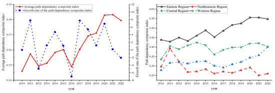
Figure 1.
Time characteristics of the transportation infrastructure path dependence composite index from 2010 to 2022.
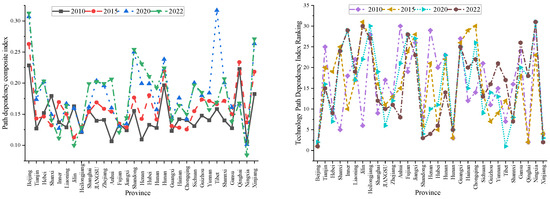
Figure 2.
Spatial characteristics of the comprehensive Index of path dependence of transportation infrastructure in 2010, 2015, 2020 and 2022.
From the composite index, the degree of carbon locked path dependence shows a spatial and temporal difference of ‘high in the east and low in the west, high in the north and low in the south’. Eastern provinces such as Shandong and Guangdong continue to rise in the composite index (from 0.1555 in 2010 to 0.2542 in 2022 in Shandong), indicating the solidifying trend of high-carbon path dependence on transport infrastructure. This is because the eastern region is economically developed, and the transport infrastructure construction started early and on a large scale, and in the long-term development process, various factors such as technology, economy, and system are intertwined, forming a deep dependence on the high-carbon path. Despite the economic and technological advantages of the eastern region, due to the large inertia of the existing development model, it faces many difficulties and challenges in promoting the low-carbon transformation of transport infrastructure, leading to the continuous solidification of high-carbon path dependence. Western regions such as Ningxia and Gansu have lower composite indices, with Ningxia at 0.0845 in 2022. This indicates that western regions have not yet formed a deep, high-carbon path dependence in the process of transport infrastructure construction as in the eastern regions. With relatively lagging economic development, a relatively small scale of transport infrastructure construction, and a relatively flexible development model, the western region has a certain latecomer’s advantage in low-carbon transition. However, Tibet has an outlier (0.3169) in 2020, which may be related to the seriousness of missing data. The fluctuation of the composite index in the northeast region is small, such as 0.129 in 2022 for Heilongjiang. This indicates that the carbon locked path dependence structure of transport infrastructure in the northeast region is relatively stable. The relatively slow pace of economic development in the northeast region and the scale and speed of transport infrastructure construction have not changed much, and the progress in technological innovation, economic restructuring, and institutional reform has been relatively slow, which makes it difficult to break the existing pattern of high-carbon path dependence, resulting in the degree of path dependence remaining at a relatively stable level.
From the perspective of time series, the development trends of low-carbon transformation of transportation infrastructure in different regions reflect the process and challenges of low-carbon transformation of transportation infrastructure in different regions. Regions with rising composite indices indicate that they have encountered greater obstacles in the process of low-carbon transformation, that high-carbon path dependence is increasing, and that they need to accelerate technological innovation, economic restructuring, and institutional reforms in order to realize the low-carbon development of their transport infrastructures. Regions with smaller fluctuations need to actively seek breakthroughs and accelerate the pace of transformation to break the existing stable but high-carbon development pattern so as to avoid facing more severe carbon emission pressure in the future. Regions with lower indices should make full use of their advantages, plan ahead, and formulate scientific and reasonable low-carbon development strategies to avoid falling into the predicament of high-carbon path dependence.
3.1.2. Spatial Characteristics of Path Dependence
Based on the data of the path dependence composite index of each province in 2010, 2015, 2020, and 2022, the spatial visualization of the institutional path dependence index was carried out by ArcGIS 10.2 (Figure 3), and the spatial characteristics of China’s path dependence composite index were summarized and analyzed according to the classification of the five levels of intervals (low value: 0.000–0.150; medium-low: 0.151–0.200; medium: 0.201–0.250; medium-high: 0.251–0.300; high-value: >0.300) to summarize and analyze the spatial characteristics of the comprehensive index of path dependence in China.
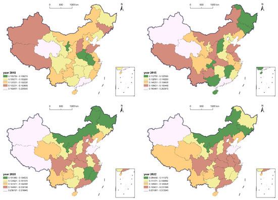
Figure 3.
Spatial distribution of China’s inter-provincial path dependence composite index in 2010, 2015, 2020, and 2022.
Long-term high levels of the path dependence composite index in provinces such as Beijing and Xinjiang reflect the strong technological, institutional, and economic lock-in effects of their established transport infrastructure networks (e.g., fuel logistics systems and energy transport corridors). The comprehensive index of path dependence in central and eastern provinces such as Shandong and Henan have risen significantly, reflecting the enhanced path dependence of transportation infrastructure construction during the process of industrialization and urbanization. Ningxia, Jilin, and other provinces continue to have a low path dependence index or benefit from policy intervention and latecomer advantages. Tibet’s traditional technological path dependence is reinforced by its frontier transport strategy (e.g., the Sichuan-Tibet railway). The path dependence index has been increasing year by year but remains at a medium dependence level. Anhui’s path dependence index is at a medium level but rising year by year, reflecting the solidifying effect of transport infrastructure networks in the transfer of industries from central China. Qinghai’s path dependence is at a low to medium level, and the index is decreasing year by year, probably due to the clean energy policy that promotes the substitution of transport technologies, and Guangdong’s path dependence is at a medium level, increasing from a low to medium level in 2010, and increasing year by year to 2022. From an overall perspective, in 2010 and 2015, high-value areas are concentrated in the northwest (Xinjiang and Qinghai) and Beijing-Tianjin-Hebei (Beijing and Tianjin), with generally low values in the central and western parts of the country; in 2020 and 2022, high-value areas in the east (Shandong and Jiangsu) are spreading to the central part of the country (Henan and Anhui), and high-value areas in the northwest (Xinjiang) continue to be strengthened, while low-value areas in the northeast (Jilin) are further solidified.
3.2. Path Dependency Determination and Lock Type
By the Pearson correlation coefficient method, the degree of path dependence at different stages of the region is determined by type, and the type of path dependence locking (e.g., technological locking, economic locking, institutional locking, etc.) is clarified for each region, and the results are shown in Table 4 and Table 5.
Table 4.
Structural path dependence results.
Table 5.
Path-dependent locking type determination result.
The eastern region shows medium dependence in stages I and II with a correlation coefficient of 0.723 * (p < 0.05), which is at a medium level of dependence, and high levels of dependence in stages II and III and III and IV, with correlation coefficients of 0.876 ** (p < 0.01) and 0.845 ** (p < 0.01), respectively, and the northeastern region is very highly dependent in the various stages; the Pearson’s coefficient for the first and second stages is 0.961 ** (p < 0.01), reaching a very high degree of dependence, while the second and third stages are 0.897 ** (p < 0.01), and the third and fourth stages are 0.951 ** (p < 0.01), all of which are in a state of high dependence. The central region also shows strong path dependence characteristics, with Pearson coefficients of 0.954 ** (p < 0.01), 0.803 ** (p < 0.01), and 0.818 ** (p < 0.01) for the three phases, respectively, and transitioning from very high to high dependence. The western region shows moderate dependence in the first and second stages (coefficient 0.691 *, p < 0.05) and then reaches high dependence in the next two stages (coefficient 0.882 ** in the second and third stages and coefficient 0.856 ** in the third and fourth stages, both p < 0.01). As a result, it can be seen that the path dependence of the carbon locked structure of transport infrastructure in each region of China is increasing over time.
From the perspective of lock-in types, the eastern region is in the first and second stages in terms of technology and economy, turns to full lock-in in the second and third stages, and is in the third and fourth stages in terms of economy and system. Research shows that initially, economic and technological factors hindered the low-carbon transformation of transportation infrastructure. However, as high-carbon systems solidified and the degree of lock-in deepened, technological innovation achieved certain success thanks to the guidance of low-carbon policies. The northeastern region is fully locked in all three stages, reflecting that the region’s technological, economic, and institutional systems are fully trapped in high-carbon path dependence and that this dependence is highly persistent. The central region is fully locked in the first and second stages, the second and third stages, and the third and fourth stages are transformed into institutional lock-in. After a certain amount of development, the technological and economic systems in the center of the country have achieved some success in their transformation, but the lagging behind of the institutional system is still an important factor hindering low-carbon development. The western region is techno-economically locked in the first and second stages, the second and third stages, and all locked in the third and fourth stages. This indicates that in the early stages of development in the western region, technological and economic factors dominated the formation of high-carbon path dependence and that the influence of institutional factors gradually came to the fore as time went by.
3.3. Characterization of Trends in the Dynamic Evolution of Path Dependence
3.3.1. Kernel Density
The kernel density estimation results in Figure 4 reveal the spatial and temporal characteristics of the carbon locking path dependence of transport infrastructure and the dynamic evolution law. From the distribution of the kernel density curve, during the period of 2010–2025, the center of the curve shows a fluctuating trend of ‘shifting to the right and then shifting to the left’: the main peak position shifted from 0.18 to 0.32 in 2010–2015, which indicates that the intensity of carbon path dependence has increased significantly; after 2015, driven by the ‘dual-carbon’ policy, the center of the curve shows a significant increase in intensity. After 2015, driven by the ‘double carbon’ policy, the center of the curve gradually shifted to the left, mapping the acceleration of the carbon unlocking process at the national level. The kernel density curve always maintains a ‘double-peak’ pattern, with the main peak on the left (low-dependence area) and the secondary peak on the right (high dependence area), and the height of the secondary peak continues to decline after 2016, indicating that the agglomeration effect of high-carbon locked provinces is weakening, but the ‘double-peak differentiation’ pattern between regions still exists. This indicates that the concentration effect of high-carbon locked provinces is weakening, but the pattern of ‘double peak differentiation’ between regions still exists. The right trailing phenomenon shrinks significantly after 2020, reflecting that the intensity of carbon locking in high dependence provinces such as Inner Mongolia and Shanxi decreases faster than that in the eastern region, and the absolute regional differences tend to converge.
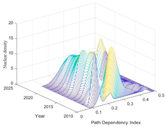
Figure 4.
Distribution of path-dependent kernel density.
3.3.2. Analysis of Overall Heterogeneity of Path Dependence
From Figure 5, it can be seen that from 2010 to 2022, the overall Gini coefficient of the composite index of path dependence shows the characteristic of ‘fluctuating upward’, and the overall Gini coefficient from 2010 to 2014 decreased from 0.084 to 0.074, and the regional differences in the dependence on the path of carbon locking have narrowed, which may be related to the convergence of policies or the diffusion of technology in the early period. From 2015 to 2021, the overall Gini coefficient fluctuated between 0.065 and 0.087, peaking at 0.087 in 2016, reflecting the contradiction between technological lock-in and policy differentiation between regions, and in 2022, the Gini coefficient soared to 0.097, the highest value in the 13-year period, indicating that the spatial heterogeneity of carbon locked path dependence has increased significantly, and regional differentiation has intensified.
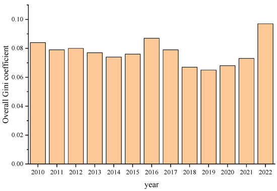
Figure 5.
Overall Gini coefficient of carbon locked path dependence for transport infrastructure.
3.3.3. Analysis of Regional Endogeneity of Path Dependence
As can be seen from Figure 6, the carbon locking path dependence of transport infrastructure shows different spatial heterogeneity in the four major regions: east, central, west, and northeast. Overall, the composite path dependence index of the four regions diverges in fluctuation, in which the eastern region faces the double lock of technology and system, the central region is constrained by the transfer of high-carbon industries and the lack of green finance, the western region seeks a balance between ecological protection and infrastructure demand, and the northeastern region is caught in the predicament of the decline of traditional industries and the lack of innovation power. In the future, the spatial polarization effect of path dependence needs to be gradually weakened through precise regional policies.
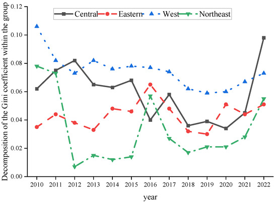
Figure 6.
Dagum Gini coefficient by region.
3.3.4. Analysis of Interregional Heterogeneity in Path Dependence
From Figure 7, the composite index of carbon locking path dependence of transport infrastructure among the four major regions of China shows significant spatial heterogeneity from 2010 to 2022. Overall, inter-regional differences are gradually narrowing in fluctuations, but the carbon locking contradictions in the east-west and east-central regions remain prominent, with technological dependence and economic dependence becoming the main driving factors, while the cross-influence of institutional dependence shows differentiated characteristics among different regions.
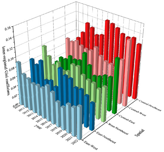
Figure 7.
Interregional Gini coefficients.
3.3.5. Sources of Heterogeneity and Contribution Rates
Figure 8 reflects the sources and contributions of carbon locked path dependence heterogeneity in transport infrastructure, and the sources of differences can be decomposed into four dimensions: path dependence composite index, technological path dependence, economic path dependence, and institutional path dependence, and the changes in the contributions of each dimension reveal the evolution of the formation mechanism of the differences in carbon locked path dependence. The results of spatial decomposition of heterogeneity show that intra-regional differences (intra-group Gw), inter-regional differences (inter-group Gb), and hyper-variable density (Gt) show significant differentiation characteristics in different dimensions.
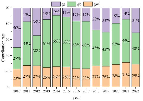
Figure 8.
Path dependence composite index contributions.
3.4. Panel Quantile Regression Results
According to the measurement results of the carbon lock path dependence index of transportation infrastructure, the degree of path dependence is divided into three grades: low, medium, and high. The digits of 0.35, 0.55, and 0.9 correspond to the low, medium, and high path dependence areas, respectively. The regression results are shown in Table 6 below, and the trend of the regression coefficients for different quantile points is shown in Figure 9 below. Grey areas are used to indicate the confidence intervals (95% confidence intervals) of the regression estimation results for each quantile.
Table 6.
Overall quartile regression results.
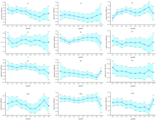
Figure 9.
Trend of regression coefficients for overall quartiles.
From the regression coefficients of each influential factor in the table, it can be seen that the estimated coefficients of each variable in the panel quartile regression model and the base regression model OLS influence the same direction basically, but there are large differences in the degree of influence of each influential factor in different quartiles, which is consistent with the conclusion of the previous hypothesis.
In the technology dimension, the regression coefficients of traditional technology inertia (T1) and technology transformation cost (T3) are positive, proving that traditional technology inertia exacerbates the carbon locking path dependence of transport infrastructure, of which T3 is the key constraint. The regression coefficient of low-carbon technological innovation (T2) is negative, indicating that T2 inhibits the creation of carbon locked path dependence in transport infrastructure.
In the economic dimension, the regression coefficients of sunk costs (S1), economies of scale (S2), and the degree of energy consumption (S3) are positive, i.e., they consistently have a positive effect on the generation of carbon locking path dependence of transport infrastructure and are not affected by the regulation of the degree of path dependence. The large coefficient of S2 indicates that it is a key factor in the economic system that affects the carbon locking path dependence of transport infrastructure, which further indicates that, with the development of transport infrastructure, the carbon locking path dependence of high-carbon infrastructure will be reduced. infrastructure development, the carbon locking path dependence is inevitable with the increase of high-carbon infrastructure.
In the institutional dimension, the degree of government intervention (R1) and low-carbon institutional lag (R3) have an inhibitory effect on the carbon locked path dependence of transport infrastructure, indicating that the institutional restructuring in the state of high intensity path dependence is more effective in governance. The regression coefficient of high-carbon institutional rigidity (R2) is positive and has the greatest influence compared with R1 and R3, highlighting the ‘rebound effect’ of institutional stickiness in the locked-in state caused by extreme path dependence.
As can be seen from the trajectories of the regression coefficients of T1, T2, and T3 in the figure, the trajectories of the influencing factors of the technological subsystem exhibit nonlinear characteristics, and the influence of technological elements on path dependence exhibits significant stage characteristics. As can be seen from the trajectories of the regression coefficients of S1, S2, and S3 in the figure, the influences of the economic factors in the economic subsystem show strong stability, but there are still significant differences between different variables. As shown by the trajectories of the regression coefficients of R1, R2, and R3, there is a reversal effect in the institutional system, and the direction and intensity of the role of institutional elements show significant heterogeneity of the sub-systems. The effect of low-carbon awareness level (LCD) shows a ‘bell-shaped’ curve, indicating that the enhancement of public low-carbon awareness has a significant facilitating effect on the cracking of medium path dependence. The inhibitory effect of the level of economic development (LED) continued to increase with increasing quantile points, suggesting the existence of a saturation threshold for the emission reduction effect of economic growth, while the effect of population density (LPD) was never statistically significant (p > 0.1), suggesting that this variable may be mediated and absorbed by other factors.
4. Discussion
With the above path dependence index measurements and path dependence and lock-in types derived from Pearson correlation coefficients and panel quantile regression results, the following discussion is made.
1. The changing trend of the comprehensive index of path dependence in different regions reflects the process and challenges of the low-carbon transformation of their transportation infrastructure. Regions with rising comprehensive indices encounter significant obstacles in the process of low-carbon transformation, and their dependence on high-carbon paths has intensified. They need to accelerate technological innovation, economic structural adjustment, and institutional reform to achieve low-carbon development of transportation infrastructure. Regions with smaller fluctuations need to actively seek breakthroughs and accelerate the pace of transformation to break the existing stable but high-carbon development model so as to avoid facing more severe carbon emission pressure in the future. Regions with lower indices should make full use of their advantages, plan ahead, and formulate scientific and reasonable low-carbon development strategies to avoid falling into the predicament of high-carbon path dependence.
2. By the type of structural path dependence and locking, the interconnection and influence of the transport infrastructure construction in the eastern region at the system level of technology, economy, and system is increasing, the path dependence effect is more and more significant, and the high-carbon development mode is gradually solidifying, and the low-carbon transformation is facing a greater challenge. The structural path dependence of carbon locking of transport infrastructure in the northeast is very stable, and the past development trajectory has had a deep impact on the present and the future, and the slow adjustment of economic structure, insufficient technological innovation, and lagging institutional reform are intertwined with each other, which makes it difficult to make a low-carbon transition in transport infrastructure. The central region has gradually formed a relatively stable development model in the process of transportation infrastructure construction. However, this model has to some extent limited the flexibility of low-carbon transformation and requires more efforts in promoting technological innovation, optimizing the economic structure, and improving the institutional system. The degree of path dependence of carbon locking in transport infrastructure in the western region is gradually deepening, and with the expansion of regional economic development and the scale of transport infrastructure construction, if the development strategy is not adjusted in a timely manner, it will face more and more severe pressure of low-carbon transformation.
5. Conclusions
This study takes transport infrastructure as an example to study the path-dependence effect in carbon locking. Based on the panel data of 31 provinces in China, the study measures the path dependence of carbon locking by constructing a system of measurement indexes and introduces a panel quantile regression model for the first time to analyze its influencing factors. The following conclusions are drawn:
1. The results of the path dependence index show that the degree of carbon lock-in path dependence of China’s transportation infrastructure is relatively high in economically developed and resource-intensive regions, and the path dependence of each system varies greatly. There is a significant difference between technical path dependence and overall path dependence. The overall path dependence characteristics are basically the same, but the economic path dependence shows the spatial feature of “high in resource-rich provinces and low in developed provinces”, and the institutional path dependence shows the obvious feature of “policy-driven fluctuations”.
2. The results of structural path dependence derived from Pearson’s correlation coefficient show that in eastern regions, it is evidenced by Pearson correlation increases from 0.723 (Stage I–II) to 0.876 ** (Stage II–III), while western regions show similar escalation (0.691 * → 0.882). Contrastingly, central regions demonstrate measurable decline from 0.954 to 0.803 ** across transitional stages, corroborated by an 18% reduction in institutional inertia metrics. Northeastern provinces maintain extreme lock-in stability (r ≥ 0.897 ** throughout stages), with dependency coefficients exceeding 0.95 in two transition phases.
3. The results of the quantile panel regression show that the influence of technological factors on path dependence presents significant stage characteristics. The strength of traditional technological inertia (T1) shows a ‘U-shaped’ curve of decreasing and then increasing as the degree of path dependence rises, while low-carbon technological innovation (T2) shows the characteristics of an ‘intermediate window of opportunity’, and the cost of technological transformation (T3) shows a ‘wave-shaped’ curve, which is influenced by the market to a greater extent. Low-carbon technology innovation (T2) shows the characteristic of ‘intermediate window of opportunity’, and technology transformation cost (T3) shows ‘wave shape’, which is influenced by the market; the influence of economic factors shows strong stability, but there are still significant differences between different variables. The sunk cost (S1) and the degree of energy consumption (S3) on the path dependence impact, by the quartile of the influence, are not big; economies of scale (S2) of the trajectory of the role of the first decline and then rise of the ‘shallow U-shaped’; institutional system have a reversal effect; the institutional elements of the direction of the role of the strength of the quartile of the performance of the significant heterogeneity of the quartile. The influence of government intervention (R1) gradually increases from the weak negative direction in the low quartile, while the rigidity of the high-carbon system (R2) shows a ‘J-type’ rebound, and the influence of the lag of the low-carbon system (R3) is relatively weak, with a significant negative effect only in the 0.1 and 0.55 quartiles (p < 0.05), and the maximum inhibitory strength of its −0.009, indicating that the low-carbon system has a reversal effect, and the direction and strength of the elements of the system show significant heterogeneity. 0.009, indicating that there is a specific ‘window of opportunity’ for low-carbon policies.
Author Contributions
Conceptualization, Y.Z. and Y.C.; methodology, Y.Z.; software, K.L.; validation, Y.Z., Y.C. and K.L.; formal analysis, K.L.; investigation, Y.W. and C.M.; resources, Y.C.; data curation, K.L. and C.M.; writing—original draft preparation, Y.Z.; writing—review and editing, Y.C.; visualization, K.L. and C.M.; supervision, Y.C.; project administration, Y.C.; funding acquisition, Y.Z. and Y.Z. All authors have read and agreed to the published version of the manuscript.
Funding
This research was funded by National Natural Science Foundation of China (No. 71774051) and the Postgraduate Scientific Research Innovation Project of Hunan Province (No. CX20210753).
Data Availability Statement
Some or all data, models, or code that support the findings of this study are available from the corresponding author upon reasonable request.
Conflicts of Interest
The authors declare no conflicts of interest.
References
- Xiao, F.Y.; Pang, Z.Q.; Yan, D.; Kong, Y.; Yang, F.J. How does transportation infrastructure affect urban carbon emissions? an empirical study based on 286 cities in China. Environ. Sci. Pollut. R. 2023, 30, 10624–10642. [Google Scholar] [CrossRef] [PubMed]
- Ji, K.K.; Yang, Q.; Dong, L.; Lin, Z.P.; Ji, K.L.; Zhang, T.; Liu, X.X. Transportation development paths in 30 provinces of China in the context of carbon quota allocation. J. Transp. Geogr. 2025, 123, 104148. [Google Scholar] [CrossRef]
- Liu, Z.H.; Xiong, H.T.; Yang, G.L. Transportation sector’s carbon emission pressure in Chinese provinces during carbon peak. Transp. Res. D Transp. Environ. 2025, 141, 104606. [Google Scholar] [CrossRef]
- Wang, L.J.; Du, K.R.; Shao, S. Transportation infrastructure and carbon emissions: New evidence with spatial spillover and endogeneity. Energy 2024, 297, 131268. [Google Scholar] [CrossRef]
- Li, J.J.; Wang, P.X.; Ma, S. The impact of different transportation infrastructures on urban carbon emissions: Evidence from China. Energy 2024, 295, 131041. [Google Scholar] [CrossRef]
- Waisman, H.D.; Guivarch, C.; Lecocq, F. The transportation sector and low-carbon growth pathways: Modelling urban, infrastructure, and spatial determinants of mobility. Clim. Policy 2013, 13, 106–129. [Google Scholar] [CrossRef]
- Dong, K.Y.; Jia, R.W.; Zhao, C.Y.; Wang, K. Can smart transportation inhibit carbon lock-in? The case of China. Transp. Policy 2023, 142, 59–69. [Google Scholar] [CrossRef]
- Cheng, Z.L.; Li, Y.L.; Zhao, L.J.; Zeng, M.J.; Shi, Z.; Wen, F.S. Transportation carbon emission structural lock-in and subsidy mechanism design in the “Belt and Road Initiative”. Transp. Policy 2025, 162, 424–442. [Google Scholar] [CrossRef]
- Yun, C.; Xianjun, C.; Xiaoya, S.; Xinyan, S. Barrier hacking level analysis of carbon locking for transportation infrastructure. J. Railw. Sci. Eng. 2024, 21, 4277–4287. [Google Scholar] [CrossRef]
- Chen, Y.; Shi, M.; Ma, C. Spatial and temporal evolution of coupling effect of carbon locking system in provincial transportation infrastructure. J. Railw. Sci. Eng. 2023, 20, 1127–1138. [Google Scholar]
- Jingke, H.; Yutong, L.; Yuxin, C. A spatiotemporal analysis of carbon lock-in effect in China’s provincial construction industry. Resour. Sci. 2022, 44, 1388–1404. [Google Scholar]
- Niu, H.; Liu, Z. Measurement on carbon lock-in of China based on RAGA-PP model. Carbon. Manag. 2021, 12, 451–463. [Google Scholar] [CrossRef]
- Niu, H.; Liu, Z. Construction of measurement indicator system of China’s carbon lock-in effect and its empirical analysis. Ecol. Econ. 2021, 37, 22–27. [Google Scholar]
- Liu, M.; Chen, Y.; Han, Z.; Wu, Z. Transition Paths for Thermal Power Generation under Carbon Lock-in Constraints. Sci. Technol. Manag. Res. 2023, 43, 241–250. [Google Scholar]
- Haiya, C. Analysis on the path of decomposition and release of carbon lock industry in China. J. Beijing Jiaotong Univ. (Soc. Sci. Ed.) 2018, 17, 44–51. [Google Scholar]
- Tao, W.; Weng, S.; Chen, X.; Malin, S. Breaking the inertia of traditional economic development: Does network infrastructure construction achieve urban carbon unlocking? Sustain. Cities Soc. 2025, 121, 106197. [Google Scholar] [CrossRef]
- Shao, Z.; Li, K.; Li, M. Coordination Effect and Interaction Response of Carbon Locking System of Transport Infrastructure under the Coupling Perspective: An Empirical Analysis Based on Municipal Panel Data in Shandong Province. Ecol. Econ. 2025, 41, 29–37. [Google Scholar]
- Cao, Y.; Wu, H.; Wang, H.B.; Liu, D.Y.; Yan, S.Q. Potential Effect of Air Pollution on the Urban Traffic Vitality: A Case Study of Nanjing, China. Atmosphere 2022, 13, 1592. [Google Scholar] [CrossRef]
- Mi, Z.; Zhou, C.; Zhu, F.; Zeng, G. The path dependence and relationship change of ecological civilization construction: Based on the panel data analysis of prefecture-level cities in the Yangtze River Economic Belt from 2003 to 2015. Geogr. Res. 2018, 37, 1915–1926. [Google Scholar]
- Schindler, M.; Dionisio, R. A framework to assess impacts of path dependence on urban planning outcomes, induced through the use of decision-support tools. Cities 2021, 115, 103256. [Google Scholar] [CrossRef]
- Da, L.; Shaowen, Z. Rubber dependence and its influencing factors in rubber producing areas—Based on the survey data of 612 rubber farmers in Xishuangbanna. Trop. Geogr. 2020, 40, 1085–1093. [Google Scholar] [CrossRef]
- Anisimov, O.; Smirnova, M.; Dulko, I. Establishment of a New Planning System in Ukraine: Institutional Change Between Europeanization and Post-Socialist Path Dependence. Plan. Theory Pract. 2024, 25, 482–501. [Google Scholar] [CrossRef]
- Loren, S. Challenging Institutional Path Dependence Through Field Configuring Events: Exploring the Collective Institutional Entrepreneurship of the Sustainable Stock Exchanges Initiative. Corp. Gov. 2024. [Google Scholar] [CrossRef]
- Huggins, R.; Stuetzer, M.; Obschonka, M.; Thompson, P. Historical industrialisation, path dependence and contemporary culture: The lasting imprint of economic heritage on local communities. J. Econ. Geogr. 2021, 21, 841–867. [Google Scholar] [CrossRef]
- Chi, J. Exploring the drivers of ecological footprint: Impacts of road transportation infrastructure, transport tax, and environment technologies. Int. J. Sustain. Transp. 2024, 18, 920–934. [Google Scholar] [CrossRef]
- Zhang, Z.; Song, P. Regional Differences in the Level of Green Finance Development in Chinese Cities and the Evolution in Time and Space. Stat. Decis. 2024, 40, 127–132. [Google Scholar] [CrossRef]
Disclaimer/Publisher’s Note: The statements, opinions and data contained in all publications are solely those of the individual author(s) and contributor(s) and not of MDPI and/or the editor(s). MDPI and/or the editor(s) disclaim responsibility for any injury to people or property resulting from any ideas, methods, instructions or products referred to in the content. |
© 2025 by the authors. Licensee MDPI, Basel, Switzerland. This article is an open access article distributed under the terms and conditions of the Creative Commons Attribution (CC BY) license (https://creativecommons.org/licenses/by/4.0/).