Article

Developing an Alternative Calculation Method for the Smart Readiness Indicator Based on Genetic Programming and Linear Regression

1
Faculty of Mechanical Engineering, University of Maribor, 2000 Maribor, Slovenia
2
Štore Steel d.o.o., Železarska cesta 3, 3220 Štore, Slovenia
3
Faculty of Mechanical Engineering, University of Ljubljana, Aškerčeva cesta 6, 1000 Ljubljana, Slovenia
4
College of Industrial Engineering, Mariborska cesta 2, 3000 Celje, Slovenia
*
Author to whom correspondence should be addressed.
Buildings 2025, 15(10), 1675; https://doi.org/10.3390/buildings15101675
Submission received: 9 April 2025 / Revised: 8 May 2025 / Accepted: 9 May 2025 / Published: 15 May 2025
(This article belongs to the Special Issue Advanced Research on Smart Buildings and Sustainable Construction)

Abstract

The European Union is planning to introduce a new tool for evaluating smart solutions in buildings—the Smart Readiness Indicator (SRI). As 54 energy efficiency categories must be evaluated, the triage process can be long and time-intensive. Altogether, 228 data points (or inputs) about the smartness of the buildings are required to complete the evaluation. The present paper proposes an alternative calculation method based on genetic programming (GP) for the calculation of Domains and linear regression (LR) for the calculation of Impact Factors and the total SRI score of the building. This novel calculation requires 20% (Domain ventilation and dynamic building envelope) to 75% (Domain cooling) fewer inputs than the original methodology. The present study evaluated 223 case study buildings, and 7 genetic programming models and 8 linear regression models were generated based on the results. The generated results are precise; the relative deviation from the experimental data for Domain scores (modelled with GP) ranged from 0.9% to 2.9%. The R2 for the LR models was 0.75 for most models (with two exceptions, with one with a value of 0.57 and the other with a value of 0.98). The developed method is scalable and could be used for preliminary and portfolio-level screening at early-stage assessments.

1. Introduction

The Green Deal defined the transformation of the European energy market in December 2019. Due to the policies related to it, the European energy market needs to be founded on the principles of energy security, energy efficiency, decarbonisation, research, innovation, and competitiveness [1]. Energy-efficient buildings are integral to the energy frameworks established in Europe. Worldwide, buildings account for 30% of the total final energy consumption [2]. In Europe, the consumption of buildings represents 40% of the final energy [3]. Furthermore, 75% of the buildings in the EU are still energy inefficient [4]. Therefore, EU Member States should strive for a cost-effective balance between decarbonising the energy supply and reducing the final energy consumption [5]. Swift advancement is essential to attain superior construction and extensive energy refurbishments in edifices that diminish the industry’s total energy requirement and carbon density [2]. An increase is needed in renewable energy sources [6]. One of the essentials for the clean energy revolution is energy-efficient buildings.
In the European Energy Performance of Buildings Directive (EPBD), from May 30th, 2018, the idea of a new tool for promoting energy efficiency was presented for the first time. This tool is called the Smart Readiness Indicator (SRI). The SRI was developed as a mechanism to evaluate the ability of buildings to incorporate information and communication technologies (ICT) [5]. Therefore, building automation has been receiving greater attention lately. A more thorough integration of building automation systems and additional advanced technologies within the building sector is essential [7]. Building automation systems possess the capability to decrease energy usage and enhance building functionality, oversight and upkeep, while simultaneously elevating the satisfaction levels of occupants [8]. Different stakeholders (building users, owners, investors, etc.) need to be informed about the added value provided by ICT in buildings [9].
The SRI aims to assess the following aspects of the technological readiness of buildings:
  • The ability to respond adaptively to the demands of the occupants.
  • The ability to facilitate maintenance and ensure optimal performance.
  • The ability to adapt in response to the energy grid circumstances [10].
A “market pull” and a “market push” are needed for the transformation of the energy market [6]. The intention of the SRI is to encourage comprehension of the positive aspects of smart buildings with respect to energy efficiency. It ought to encourage cooperation between the energy, construction, and ICT sectors in the building industry [11]. All parts of the real-estate market must cooperate in a coordinated approach [12]. The Smart Readiness Indicator endeavours to accomplish this objective by integrating the requirements of the occupants, facilities and energy grids in accordance with the vision for a sustainable energy transition [13]. The result should be an optimised mix of various energy sources, user occupancy, and grid flexibility [14]. It is expected that the SRI will be particularly beneficial for large buildings with a large energy demand [15]. The implementation of modern energy systems consisting of battery storage systems, photovoltaic production, and flexible loads through cooperative and individual optimisation scenarios would be accelerated with the help of the SRI [16]. Furthermore, the SRI could accelerate the implementation of the smart cities’ vision [17].
The SRI was previously evaluated in different ways. Various authors [18,19,20,21,22,23] believe that the SRI will function as a supplement to the energy performance certificates (EPCs). Others [9,19,24,25] pointed out that the triage process (the process in which the data of the building is collected and later evaluated so that the SRI score can be calculated) is too subjective and can hardly be replicated. Some researchers claim that the buildings must have identical properties for consistent and comparable results [26]. A study pointed out that the SRI is not suitable for buildings under monument protection conditions [27]. Other researchers pointed out that the results of the SRI evaluation should be used alongside other performance measures to fully understand the energy and functional performance of smart buildings [28]. A study conducted on 59 high-performance buildings in South Tyrol, Italy, came to the conclusion that the readiness levels varied across categories and that there was no direct correlation between the SRI and the energy performance [29].
Some studies propose the combination of quantitative and qualitative measures that would make the triage process more objective. By defining clear indicators and standards for different impact areas, the creation of standardised SRI scores across various building types and climates would be possible [30]. The idea of combining SRI with custom KPIs and minimum thresholds also appears in another study [31]. Also, a study conducted on Italian case studies proposed a tailored approach by adjusting the service inclusion and weighting factors. Also, the final SRI score would improve significantly [32]. Some authors have proposed a hybrid methodology that would integrate SRI assessments into traditional EN 16247 [33] energy audits. This would enable a more comprehensive evaluation of both energy efficiency and a building’s readiness for smart technologies [34]. The authors of a comparable study also came to similar conclusions [35].
There are papers suggesting the usage of digital twins and BIM. This solution would help in reducing subjectivity and provide more reliable and comparable scores across different building types, systems and climate zones [36]. When comparing the SRI with the EN ISO 52120 [37], authors also advocate for the use of BIM and digital twin technologies to improve the accuracy of SRI evaluations. The study also underlines that regional differences in technical systems can influence the SRI outcomes [38].
The European Union is in the middle of the Renovation Wave, which aims to renovate 35 million buildings by 2030 [39]. The EU Renovation Wave Strategy aims to (at least) double the building renovation rate by 2030, with a focus on improving energy performance and digital readiness, including SRI implementation [39]. The required funding is supported by the dedicated EU Green Deal Investment Plan [40].
The original SRI evaluation method is time-consuming, as it often requires multiple site visits, coordination with building staff (such as maintenance personnel or energy managers), the collection of technical documentation and blueprints, and finally, manual data entry into the official SRI calculation Excel tool. Therefore, this method is hard to apply on a large scale. Considering this, there is a clear need for a new, alternative method of calculating the SRI that reduces the needed inputs and keeps the desired accuracy. The present paper uses genetic programming (GP) and linear regression (LR) for the calculation of SRI scores. Genetic programming is an evolutionary computation technique that solves problems automatically without requiring the user to know or specify the form or structure of the solution in advance. At the most fundamental theoretical level, GP constitutes a systematic, Domain-independent framework for facilitating autonomous problem-solving by computers [41]. It initiates from a generalised declaration of what must be accomplished and generates a computer program to address the problem autonomously [42]. GP is simulating natural selection and the principles of genetics, often reducing the complexity of finding solutions [43].
GP has found its place in many applications related to buildings. Studies report the usage of GP in finding the optimal window–wall ratio [44], optimising the building design to reduce HVAC (Heating, Ventilation, and Air Conditioning) demands [45] and energy costs [46], optimising space allocation problems [47], and finding alternative building designs [48]. Also, its role in solving other engineering problems was reported, such as in finding the optimal cross-sectional areas of structural members [49].
Linear regression (LR) is a robust statistical technique designed to ascertain the correlation between the independent input variables (i.e., the explanatory variables) of the system and the dependent output variable (i.e., the response of a system) [47] and to identify models with the “optimal fit” for the data [48]. In LR, the dependent variable is represented as a linear function of a set of regression coefficients and a stochastic error.
To the maximum extent of the authors’ knowledge, only a few papers have tackled the development of alternative calculation methods for the SRI. One paper is from 2019, by Markoska et al. [20], and emphasises performance testing (PTing). They claim that PTing frameworks are a solution that utilises metering and sensors for real-time performance monitoring. To work properly, a metamodel of the building is needed, with a layer of hardware abstraction that incorporates operational information, and a minimum SRI score of 23% [20]. This is also the most significant limitation that the authors highlighted. The paper, however, does not state the accuracy of the developed method.
The second paper that deals with an alternative SRI method is from 2023, by the authors Yu Ye et al. [50], and describes the development of the tool SmartWatcher©. The instrument provides a solution to assess the intelligence of buildings through the utilisation of automated natural language processing. The developers formulated a mechanism that transforms verbal data into quantitative information to evaluate smart readiness in buildings. It was examined on eight trial buildings. The outcomes indicated that the approach had potential for enhancement. The paper reported a success rate of 73.61% and a hit rate of 66.57%.
The third paper that discussed a new SRI calculation method is from 2024, by the authors Carnero et al. [51]. A novel approach (semi-automated) was presented, which evaluates SRI scores. For this it used the building information modelling (BIM) and industry foundation classes (IFC) schema. The IFC schema is a standardised, open data format that enables detailed digital descriptions of building components and systems. The study describes the following four-step process: interpretation, model preparation, execution, and reporting. The study identified and assessed 60–80% of smart-ready services, especially in HVAC and electrical systems. The authors reported time saving, improved accuracy, and a support of the wider use of digital tools in the assessment of smart solutions in buildings.
Table 1 compares this study with the three relevant papers described earlier. Unlike prior works that relied either on metadata models (Markoska et al.) [20], NLP-based interpretations (Ye et al.) [50] or BIM-based rule interpretation (Carnero et al.) [51], our approach pioneers a hybrid data-driven (GP + LR) method to assess the SRI. The method is suited for real-world and digital model SRI evaluations. Automation of the method is also planned.
In general, our research is divided into two parts. The first part focuses on developing a model to predict the SRI scores. In future research, this model will be used to read live data from real case study buildings and calculate the SRI scores which will represent a step towards automated SRI evaluation of buildings.
The paper is organised in the following manner: Section 2 describes the Methods used in our study. The experimental setup and data collection are described in Section 2.1. This is followed by research data preparation for modelling in Section 2.2. Section 3 is dedicated to modelling. Section 3.1 specifies the approach to modelling Domains, followed by a discussion on the modelling of impact factors in Section 3.2, and the comprehensive evaluation of the total SRI building score in Section 3.3. Section 4 describes the outcomes of the modelling process. The findings of Domain modelling are presented in Section 4.1, the results pertaining to the Impact Factors’ modelling are detailed in Section 4.2, and the overall SRI score of the building is presented in Section 4.3. Section 5 offers a discussion on the results of the paper and their significance. The concluding observations are articulated in Section 6. The closing remarks are also presented in Section 6.

2. Methods

GP and LR modelling are used to create prediction models that can predict the Domain scores, Impact Factors, and total building SRI score. The descriptive method is used to describe the facts and to examine and describe the results. All the terms and definitions employed in this study adhere to the official Smart Readiness Indicator (SRI) methodology as established by the European Commission, in collaboration with the SRI Support Team comprising VITO (Belgium), Waide Strategic Efficiency (Ireland), R2M Solution (France), and the Luxembourg Institute of Science and Technology (LIST) [52].

2.1. Experimental Setup and Data Collection

The study began with experimental work spanning over two years, namely 2021 and 2023, whereby 223 case study buildings were evaluated in Slovenia. The case study buildings were then classified by purpose of use according to the SRI methodology. This distribution is represented in Figure 1.
According to the SRI methodology, the case study buildings are in the southeastern region. The SRI evaluation or the triage process began with one or multiple visits to the facility, data collection about the smart systems installed in the building, document reading (plans of mechanical and electrical installations, etc.), and interviews with the facility manager(s).
The data on the buildings’ built-in systems and how systems are controlled and monitored were collected carefully. After the data collection phase, the evaluation of the SRI score was performed with the official Excel calculation tool version 4.5 provided by the SRI support team (also known as the “Clipboard method” [50]). The default Method B was used for the SRI calculation, as it suits most building types [52].

2.2. Research Design and Data Preparation for Modelling

The original SRI methodology evaluates the smartness of buildings in three different categories, namely the Domains, Impact Factors, and total SRI score of the building [51]. The subcategories of these scores are presented in Table 2.
Every category of the results analyses “the smartest” in buildings in different ways. Domains and Impact Factors have subcategories against the total SRI score, an independent score with no subcategories. The subcategories or “services”—in the terminology of the SRI methodology—have different service levels. The purpose of service levels is to find the one that describes how energy systems are managed and controlled in the building. Every service level is described in 3–5 levels (depending on the service). The categories follow one another from the simplest to the most complex. The total number of all service levels is 231, e.g., the first smart service is heating (Code H-1a). The methodology proposes 5 possible levels [52], namely “0-No automatic control”, “1-Central automatic control (e.g., a central thermostat)”, “2-Individual room control (e.g., thermostatic valves or an electronic controller)”, “3-Individual room control with communication between controllers and to BACS” (Building Automation and Control System), and “4-Individual room control with communication and occupancy detection”. For example, “level 0”—“no automatic control was labelled” H1A1, “level 1”—“Central automatic control (e.g., a central thermostat)” received the name H1A2, etc. (the complete conversion table is provided in the Appendix A).
The first step of data preparation was assigning every service level with an index. A conversion table was prepared (see Table A1, Table A2, Table A3, Table A4, Table A5, Table A6, Table A7, Table A8 and Table A9 in Appendix A) that translates the individual service levels into a shorter form that can be used in the prediction models.
The second step was to gather all the data from the experimental work in a large spreadsheet, as presented in Table 1. All 223 different case study buildings were listed in the leftmost column. The top row lists all 231 service levels (with the assigned indexes). The experimental evaluation was performed as follows: when a level described the situation in the building perfectly, it scored 1. If the level did not describe the situation, it was assigned a 0. If the building did not have a particular system installed, the Domain received a score of 2 (e.g., if a building did not have the option of charging electric vehicles, then all the levels received the score 2). The principle of how all the buildings’ evaluation data were prepared is presented in Table 3.
The next step was to develop models for individual Domains with GP.

3. Modelling

This section presents the modelling of the Domains in Section 3.1, followed by the modelling Impact Factors in Section 3.2 and the total SRI building score in Section 3.3.

3.1. Modelling Domains Using GP

The decision to select GP as the Domain modelling method was based on our positive prior experience in various engineering fields. These included solving general engineering problems [53,54] and energy optimisation problems [55,56,57], where it has provided accurate and transparent results consistently. The generated mathematical models can be inspected, analysed, and interpreted directly. The discrete input data needed for Domain modelling (0, 1, 2) were especially well-suited for GP, which excels at handling symbolic, rule-based relationships. After the Domain scores were determined, linear regression (LR) was selected for modelling the Impact Factors and total SRI because of its efficiency, straightforwardness, and clarity. Our chosen approach strikes a balanced compromise between accuracy, efficiency, and practical usability. Although more sophisticated approaches, such as random forests or SVMs, might provide marginally improved predictive precision, they generally compromise on interpretability and demand more computational power. Our chosen approach strikes a balanced compromise between accuracy on a larger scale, efficiency, and practical usability.
GP mimics the processes of natural selection. If the organism is successful in its quest for survival, its descendants will inherit its properties. The end goal of GP is to find the perfect model that describes our observed phenomenon. The fundamental working principle of GP is presented in the following Equation (1) [54]:
“t = 0
create staring population P(t)
evaluate starting population P(t)
continue
change P(t) -> P(t + 1)
evaluate P(t + 1)
t = t + 1”
These steps are repeated until the stopping criterion is met.
By crossing organisms, we are creating populations that become better and better at fitting in by solving a technical problem, i.e., developing an individual equation that represents a model that forecasts results—in our case the Domain scores.
The following basic mathematical operations were used to initiate different combinations in genes [53]:
  • “addition (+)”;
  • “subtraction (–)”;
  • “multiplication (*)”;
  • “and division (/)”.
The computer program for generating mathematical models was written in the programming language AutoLisp inside the AutoCAD CAD/CAM systems (AutoCAD Release 14, Autodesk, San Rafael, CA, USA) [53]. The generated results were saved in multiple.txt files, with a set for each Domain. The batch was selected from the dataset with the lowest relative deviation from the experimental data between the best model of the individual generation and the experimental raw data results. The following evolutionary settings were used for the GP system:
  • “tournament size for selection operation 6.0”.
  • “maximal permissible depth in the creation of the population: 30”.
  • “maximal permissible depth after the operation of crossover: 20”.
  • “reproduction probability [%]: 0.7”.
  • “crossover probability [%]: 0.2”.
  • “number of organisms: 500”.
  • “tournament selection method with tournament size: 7”.
  • “number of independent runs: 50” [54].
A total of 50 generations of models were developed for every Domain. For the winning one, we selected the last generation, since it was the most accurate. The winning models by individual Domains are presented in Equations (2)–(8). The models predicted the Domain scores with a relative deviation that is stated below. Variables (M33, H2D5, H2B3, etc.) represent the smart service level of an evaluated building. The conversion Table of indexes and services is presented in Appendix A, Table A1, Table A2, Table A3, Table A4, Table A5, Table A6, Table A7, Table A8 and Table A9.
Each index used in the model (2, 3, 4, 5, 6, 7, and 8) represents a specific smart service within the building. A corresponding conversion Table, listing all the smart services and their assigned indexes, is provided in the Appendix A. The inputs in variables are discrete values (0, 1, or 2), as described in the previous section. If the smart level is presented, the parameter receives a value of 1; if it is not, it receives a value of 0. If the smart service can-not be evaluated in the building (if the building does not have a specific system, for example), the parameter receives a value of 2. The Domain scores are calculated directly by inserting discrete values, as described earlier. The equation form of the genetic programming models is presented in Appendix B.

3.1.1. Score Prediction Model for the Heating Domain

Generation: 50 (from 50)
Equation (2) presents the model that predicted the scores for the heating Domain. The relative deviation from the experimental scores was 2.26%.
Domain Heating =
(+ (+ (+ (− (* (− H33 H2D5) H2B3) (− (+ H1C2 H31) (* (− 7.16973 (+ 5.81691 H2D1)) (* (− (− (+ (− H33 H2D2) H2B3) (− (+ H1C2 (+ (* H2D5 H1A5) H31)) (* (− 7.16973 (+ 5.81691 H2D1)) 7.16973))) (− (+ (* (− (+ (− H33 H2D2) H2B3) (− (+ H1C2 H31) (* (− 7.16973 (+ 5.81691 H2D1)) H2D2))) (− H33 H1B2)) H44) (− (* H2D5 H2B3) (− (+ H1C2 H31) (− (+ H33 (+ H1C2 H2B3)) (− (+ (+ (* H2D5 H33) (+ H1A5 (+ (* H2B1 H1A4) H33))) (+ H1A5 (+ (+ (% H2B1 H1A5) H1A4) H31))) (* (% (+ (− H33 9.66955) (− (* H2D5 H2B3) (− (+ H1C2 (− (+ H1C2 (− (* (% H2D2 (+ (* H2B1 H2D2) H2D1)) (+ H1C2 (+ (* H2D5 H1A5) H31))) H31)) (* (+ (* H2B1 H1A4) H2D1) H31))) H2D2))) (+ (− (+ H1C2 (− H31 H31)) (* (% H2D2 H2D1) H2D2)) H2D1)) H2D1))))))) H35)))) (+ (− (* H2D5 H2B3) (− (+ H1C2 (− (+ H1C2 H31) (* (− 7.16973 (+ (+ 9.66955 H2B1) (+ (% H2B1 H1A4) H2D1))) H31))) (* (− (− (+ (− H33 H2D2) H2B3) (− (+ H1C2 H31) (* (− 7.16973 (+ 5.81691 H2D1)) 7.16973))) (− (+ (* (% H1F1 H2D2) (− H33 H1B2)) H44) (− (* H2D5 H2B3) (− (+ H1C2 H31) (− (+ (* (% H2D2 (+ (* H2B1 H2D2) H2D1)) H33) (+ (% H2B1 H1A5) H2B3)) (− (+ (+ H33 (+ H1A5 (+ (* H2B1 H1A4) H33))) (+ H1A5 (+ (* H2B1 H1A4) H31))) (* (% (+ 9.66955 (− (* H2D5 H2B3) (− (% H2D2 (+ (* H44 H2D2) H31)) H2D2))) (+ H1C2 H2D1)) H2D1))))))) H1A4))) (+ 9.66955 (− (* H2D5 H2B3) (− (+ H1C2 H31) (* (% H2D2 (+ (* H2B1 H2D2) H2D1)) 5.46992)))))) H2B2) (+ 5.81691 9.83727)))

3.1.2. Score Prediction Model for the Domestic Hot Water Domain

Generation: 50 (from 50)
Equation (3) presents the model that predicted the domestic hot water Domain scores. The relative deviation from the experimental scores was 2.53%.
Domain Domestic hot water =
(* (− (+ (% (+ (% (% DHW1D1 DHW2B5) DHW1A4) (+ DHW1B1 DHW2B5)) DHW1A4) (+ (% −3.14511 DHW1B1) DHW1D3)) (− (% −3.14511 (* (% DHW1D1 DHW1A2) DHW1B3)) (− (+ DHW2B1 9.18609) DHW32))) (* (% (* (− DHW1D3 (− (% −3.14511 DHW1B3) (− (+ DHW2B1 9.18609) DHW32))) (* (% (% (% (− (* (% DHW1D1 DHW1A2) DHW1D1) DHW1A4) (% (+ DHW31 DHW2B2) DHW34)) (+ DHW2B1 DHW1D3)) (* (* DHW1A4 DHW1B1) (+ DHW31 (* (% (% DHW34 (% −3.14511 DHW1D3)) (* (* DHW1A4 DHW1B1) (+ DHW31 (+ DHW2B1 DHW2B5)))) DHW2B5)))) DHW1D3)) (* (* DHW1A4 DHW1B1) (+ DHW31 (− (+ DHW2B1 9.18609) DHW2B5)))) 3.21647)))

3.1.3. Score Prediction Model for the Cooling Domain

Generation: 50 (from 50)
Equation (4) presents the model that predicted the scores for the cooling Domain. The relative deviation from the experimental scores was 2.97%.
Domain Cooling =
(* (− (+ (− (+ C1B2 C2A1) 7.66353) (+ (* (* C1A4 (% (* (* C1A4 C1F1) C34) (+ (− C1F1 C43) (* C1A4 (+ 7.66353 C1F1))))) C43) C1F3)) (− C1D3 C1D1)) (− (+ (− (− (+ (− (+ (− C2A1 7.66353) (+ C43 (− C1F1 C1F3))) (− (* (+ C43 (− C2A1 C1F1)) C1D3) (+ C1D5 (% (* (+ (− (+ (− (% (* (* C1A4 C1F1) C34) (+ (− C1F1 C43) (* C1A4 (+ 7.66353 C2A1)))) 7.66353) (+ (+ C43 (+ C43 (− C1F1 C43))) (− C1F1 C1F3))) (− C1D3 (+ C1D5 (% (* (* C1A4 (+ (− C2A1 7.66353) (+ C43 C1F1))) C34) 7.66353)))) (+ C43 (− C2A1 C1F1))) (+ C43 C34)) 7.66353)))) (+ (− C1F1 C43) (− C1F1 C1F3))) (− C1D3 (+ C1D5 (% (+ (− C1F1 7.66353) (+ C43 (% (+ (− C1F1 7.66353) (+ C43 C34)) (+ (− C1F1 C43) (* C1A4 (+ 7.66353 (+ C43 (+ C43 C34)))))))) (+ (− C1F1 C43) (* C1A4 (+ 7.66353 (+ C43 (+ C43 C1F3))))))))) (− C1D3 (+ C1D5 (% (* (+ C1D5 C1F1) C34) 7.66353)))) (+ C43 (− C1F1 C1F3))) (− C1F1 C31))))

3.1.4. Score Prediction Model for the Ventilation Domain

Generation: 50 (from 50)
Equation (5) presents the model that predicted the scores for the ventilation Domain. The relative deviation from the experimental scores was 1.50%.
Domain Ventilation =
(+ (+ (+ (+ (* (* (% (− 8.4716 (% (− V31 −5.25128) (% (* (% V2C2 V1C5) V2D2) (+ V1C3 V1A3)))) V62) V33) V64) (− 8.4716 (% (+ (* (− (* (% V64 V33) (− V31 (% (* (% V2C2 V1C5) V2D2) (* (* (% (− 8.4716 (% (* (− V2C3 (− V1C2 V1C2)) (% (* (% V2C2 V1C5) V2D2) (+ V1C3 −5.25128))) (% (* (% V2C2 V1C5) V2D2) (+ V1C3 V1A3)))) V62) V33) V1C1)))) (% V1A2 (+ (* (− (* (− (* V61 (+ V1C3 (% (* (% V2C2 V1C5) V2D2) (+ V1C3 V2C3)))) (− V1C2 V61)) (− 8.4716 (% (− V31 (% (* (− 8.4716 (% (* (− (* V61 (+ V1C3 V2C3)) (− V1C2 V1C2)) (% (* (% V2C2 V1C5) V2D2) −5.25128)) V1C5)) V2D2) (+ V1C3 −5.25128))) (% (* (% V2C2 V1C5) V2D2) (+ V1C3 V2C3))))) V1C2) V1A5) V1A5))) V2D3) (* (% (− 8.4716 (− 8.4716 (% (− V31 −5.25128) (% (* (% V2C2 V1C5) V2D2) (+ V1C3 V1A3))))) V62) −5.25128)) (% (% (− (% V64 V1C1) (% V1A2 (% V1A2 (+ (* (* (% (− 8.4716 (% (* (− V2C3 (− V1C2 V1C2)) (% (* (% V2C2 V1C5) V2D2) (+ V1C3 −5.25128))) (% (* (% V2C2 (+ V1C3 V1C5)) V2D2) (+ V1C3 V1A3)))) V62) V33) V1A5) V2C1)))) (% (% V2D1 (+ V1A2 (− 6.96117 V2D1))) V2D2)) V1C4)))) (− (+ V64 (− 8.4716 (% (− V31 (% (* (% V2C2 V1C5) V2D2) (+ V1C3 −5.25128))) (% (* (% V2C2 V1C5) V2D2) (− 8.4716 (% (+ (* V1A5 V2D3) −5.25128) (% (% (* (+ V34 V1A3) (% V64 V2D2)) (% V2C2 (+ V64 (* (+ (* V1A5 V2D3) 1.53678) V2D2)))) 6.96117))))))) V61)) (− 6.96117 V33)) V1C2))

3.1.5. Score Prediction Model for the Lighting Domain

Generation: 50 (from 50)
Equation (6) presents the model that predicted the scores for the lighting Domain. The relative deviation from the experimental scores was 1.36%.
Domain Lighting =
(* (* (% (− L25 L1A3) (* (− (− (+ L21 (* (* (% (+ (+ L23 L23) L1A3) L1A1) 3.27069) (− L25 L1A4))) L24) L22) L1A1)) (− (− L25 L22) (+ (− (* (+ (− (− L25 L25) L23) (+ (+ L23 L23) L22)) −0.160899) (* (* (% (− L25 L1A3) L1A1) (+ L23 3.27069)) (% L24 (+ L1A4 L21)))) (− (* (+ (+ L23 L23) L22) −0.160899) (* (% (% (+ L23 L1A3) (− L25 L1A3)) L1A1) (− (+ (+ (% L24 (+ L1A4 L1A4)) L1A2) (% L22 L22)) (+ (+ L21 (− (* (+ (− L25 L23) L22) (− L22 (+ (− L25 L21) (− (* (+ (+ L23 L23) L22) −0.160899) −0.160899)))) (* (* (% (+ (+ L23 L23) L1A3) L1A1) 3.27069) (% L24 (+ L1A4 L21))))) (− L25 3.27069)))))))) (+ (% (* 3.27069 (+ (* (% L24 (+ L1A4 L1A3)) (* L1A3 (− (+ L1A1 (% (+ L23 L1A3) L22)) (* (− (− (+ L21 (− (* (+ (+ (* L1A3 (− L1A2 L1A2)) (% (% L1A2 L22) L23)) L22) (− L22 (+ (% (% L1A2 L22) L21) (− (* (+ (+ L23 L23) L22) −0.160899) −0.160899)))) (* (* (% (+ (+ L23 L23) L1A3) L1A1) 3.27069) (% L24 (+ L1A4 L1A4))))) L24) L22) L1A2)))) (% (% L1A2 L22) L24))) (+ (% L24 (+ L1A4 L1A4)) L1A2)) (% (+ L23 L22) L1A3))))

3.1.6. Score Prediction Model for the Dynamic Building Envelope (DBE) Domain

Generation: 50 (from 50)
Equation (7) presents the model that predicted the dynamic building envelope Domain scores. The relative deviation from the experimental scores was 0.92%.
Domain Dynamic building envelope =
(setq ideal ‘(+ (* (− DE41 (− 5.87984 (* DE11 DE22))) (− (+ DE44 (+ DE44 (− DE15 (+ (+ (+ (− DE42 DE44) (* (% DE22 DE11) (% DE24 DE44))) DE13) DE23)))) (+ (+ (− DE42 DE44) (* (% DE22 DE11) (% (− (+ (− DE42 DE13) (+ (− DE22 DE13) (* (% (+ (− DE42 DE13) (+ (− (* (% DE22 DE11) (% (− DE22 DE24) 5.87984)) (* DE11 DE13)) (* (% (* (− DE43 DE12) (% DE13 (* (− DE41 (− 5.87984 (* DE11 DE22))) (− (+ DE44 (+ DE44 (− DE15 (+ (+ (− DE42 DE44) DE13) DE23)))) (+ (+ DE44 DE14) (+ (+ (* DE11 (− DE22 DE13)) (+ (− DE22 DE13) DE22)) DE22)))))) (* DE11 DE11)) (− DE42 DE22)))) DE11) (+ (− DE42 DE44) DE22)))) DE24) DE14))) (+ (+ DE13 (+ (− DE22 DE13) (* (% (* (− DE43 DE12) DE22) DE11) (+ (− DE22 (+ (− DE22 DE13) DE44)) DE22)))) DE14)))) (+ (+ (− (+ (− DE42 DE13) (+ (− DE22 DE13) (* (% (+ (− DE42 DE13) (+ (− DE22 DE13) (* (+ (− DE42 DE44) (* (% DE22 DE11) (% DE24 DE11))) (− DE42 DE22)))) DE11) (+ (− DE42 DE44) DE22)))) DE13) DE22) (− DE42 DE42))))

3.1.7. Score Prediction Model for the Electricity Domain

Generation: 50 (from 50)
Equation (8) presents the model that predicted the scores for the electricity Domain. The relative deviation from the experimental scores was 2.62%.
Domain Electricity =
(− (% EL35 (% (% (% (− EL124 EL125) (* EL122 −7.29756)) (− EL82 (% EL31 EL124))) (% (− EL124 −7.29756) (− EL82 (% EL31 EL114))))) (− (− (% (% (% (− (− EL124 (% (* EL124 EL51) (% (% (− EL124 EL125) −7.29756) (− EL82 (% EL31 EL124))))) EL125) (* EL122 (* EL122 −7.29756))) (− EL82 (% EL31 − 7.29756))) (− EL82 (% EL31 EL125))) 8.69097) (− EL81 (− (+ (* EL122 EL34) (* EL122 EL41)) (* EL82 (− (− EL35 EL33) (% (* EL124 EL51) (% (% (− EL124 EL125) −7.29756) (− EL82 (% EL31 EL112))))))))))

3.2. Modelling Impact Factors Using LR

LR was used for the prediction models of the Impact Factors instead of GP. Linear regression (LR) was chosen for modelling the Impact Factors and total SRI due to its speed, simplicity, and transparency, making it well aligned with the goal of developing a practical evaluation tool. Based on initial tests with LR, the developed models proved reliable, with little deviation from experimental data (the regression statistic is described in the Results section). The process of modelling the Impact Factors was performed in Microsoft Excel, ensuring clarity and reproducibility.
The standard equation that describes the LR is as follows [57]:
a = β0 + β1 X1 + β2 X2 + … + βn Xn + ε
where:
  • a is a dependent variable (the Impact Factor);
  • X1, X2, are the independent variables;
  • β0, β1, …, βn are the coefficients (in our case, Domain scores, modelled with GP, as described in Section 3.1.1 to Section 3.1.7);
  • ε represents the error term or the intercept.
  • In our case, the standard equation for our models is as follows:
a = β1(Domain heating) X1 + β2(Domain domestic hot water) X2 + β3(Domain cooling)X3 + β4(Domain ventilation) X4 + β5(Domain lighting) X5 + β6(Domain dynamic building envelope) X6 + β7(Domain electricity) X7 + β 8(Domain EV charging) X8 + β9(Domain monitoring and control) X9 + ε
Based on the general Equation (10), the following prediction models for different Impact Factors are as follows.
Equation (11) represents the model for the prediction of the energy efficiency Impact Factor, as follows:
a1(Impact Factor Energy efficiency) = β1 0.50807 + β2 0.04754 + β3 0.0753 − β 4 0.0473 + β5 0.0652 + β6 0.0483 + β7 0.0061 + β8 0.0057 + β9 0.0452 + 22.2267
Equation (12) represents the model for the prediction of the energy and storage impact factor, as follows:
a2(Impact Factor Energy and storage) = β1 0.0326 + β2 0.95 − β3 0.0041 − β4 0.025 + β5 0.0006 − β60.032 − β7 0.0004 + β8 0.0061 + β9 0.1558−0.3229
Equation (13) represents the model for the prediction of the comfort Impact Factor, as follows:
a3(Impact Factor Comfort) = β1 0.1863 − β2 0.0062 + β3 0.1353 + β4 0.2641 + β5 0.1673 + β6 0.0856−β7 0.0366 + β8 0.00123 + β9 0.0946 + 20.2056
Equation (14) represents the model for the prediction of the convenience Impact Factor, as follows:
a4(Impact Factor Convenience) = β1 0.1650 + β2 0.0010+ β3 0.089 + β4 0.1379 + β5 0.07863 + β6 0.1065 + β7 0.0049 + β8 0.0222 + β9 0.1882 + 13.3274
Equation (15) represents the model for the prediction of the health, well-being, and accessibility Impact Factor, as follows:
a5(Impact Factor Health, well-being, accessibility) = β1 0.2561 − β2 0.0224 + β3 0.0976 + β4 0.1930 + β5 0.0957+ β6 0.10625 − β7 0.0163 − β8 0.0411 + β9 0.0976 + 9.0174
Equation (16) represents the model for prediction of maintenance and fault prediction Impact Factor, as follows:
a6(Impact Factor Maintenance and fault prediction) = β1 0.64340 + β2 0.0349 + β3 0.0276 + β4 0.0739 + β5 − 0.0305 + β6 0.0648 + β7 0.0095 − β8 0.0103 + β9 0.3043 − 2.6152
Equation (17) represents the model for the prediction of the information for the occupants Impact Factor, as follows:
a7(Impact Factor Information for the occupants) = β1 0.1858 + β2 0.0598 + β3 0.0926 − β4 0.0500 − β5 0.0106 + β6 0.08007 + β7 0.19854 − β8 0.0089 + β9 0.2087 + 10.9335

3.3. Modelling the Total SRI Score of the Building Using LR

All the Domains and all the Impact Factors impact the total SRI score of the building. Therefore, the standard equation for our model is as follows:
γ = a1(Impact Factor Energy efficiency) X1 +a2(Impact Factor Energy and storage) X2 +a3(Impact Factor Comfort) X3 + a4(Impact Factor Convenience) X4 +a5(Impact Factor Health, well-being, accessibility) X5 +a6(Impact Factor Maintenance and fault prediction) X6 +a7(Impact Factor Information for the occupants) X7 + β 1(domain heating) X8 + β 2(domain domestic hot water) X9 + β 3(Domain cooling) X10 + β 4(Domain ventilation) X11 + β 5(Domain lighting) X12 + β 6(Domain dynamic building envelope) X13 + β7(Domain electricity) X14 + β 8(Domain EV charging) X15 + β 9(Domain monitoring and control) X16 + ε
where:
  • γ is a dependent variable (the total SRI score of the building);
  • X1, X2, are the independent variables;
  • a1, a2 are the Impact Factors (using the calculation described in the previous Section 3.2 with LR);
  • β0, β1, …, βn are the domains (using the calculation described in Section 3.1.1 to 3.1.7 with GP);
  • ε represents the error term or the intercept.
  • Equation (19) represents the model for the prediction of the total SRI score of the building, as follows:
γ = a1(Impact factor Energy efficiency) 0.16614 + a2(Impact factor Energy and storage) 0.32764 +a3(Impact factor Comfort) 0.07882 + a4(Impact factor Convenience) 0.08521 + a5(Impact factor Health, well-being, accessibility) 0.08178 + a6(Impact factor Maintenance and fault prediction) 0.16470 + a7(Impact factor Information for the occupants) 0.08431 − β 1(Domain heating) 0.00110 + β2(Domain domestic hot water) 0.00229 + β3(Domain cooling) 0.00075 + β4(Domain ventilation) 0.003169 − β5(Domain lighting) 0.00025 − β6(Domain dynamic building envelope) 0.00254 − β7(Domain electricity) 0.001393 − β8(Domain EV charging) 0.000905 + β9(Domain monitoring and control) 0.00669 + 0.125126

4. Results

This Section presents the results in three sections. The results for the Domain modelling are given in Section 4.1. The results for the Impact Factors are given in Section 4.2, and the results for the total SRI score of the building are presented in Section 4.3.

4.1. Results for Domain Modelling

In total, 50 generations of models were generated with GP for each Domain. The last generation (50th) was the most accurate, as the relative deviation from the experimental data was the lowest. Therefore, the 50th generation was selected as the winning one for each Domain. Figure 2 represents the relative deviations in percentages. The relative deviations ranged from 0.92% for the lowest Domain (the dynamic building envelope Domain) to 2.97% for the highest (the cooling Domain).

4.2. Results for Impact Factor Modelling

Using the developed models in Section 3.2, the Impact Factors for all 223 case studies were calculated and are represented graphically in the multi-panel Figure 3. The regression statistic for the Impact Factors and the total SRI score is stated in Table 4.

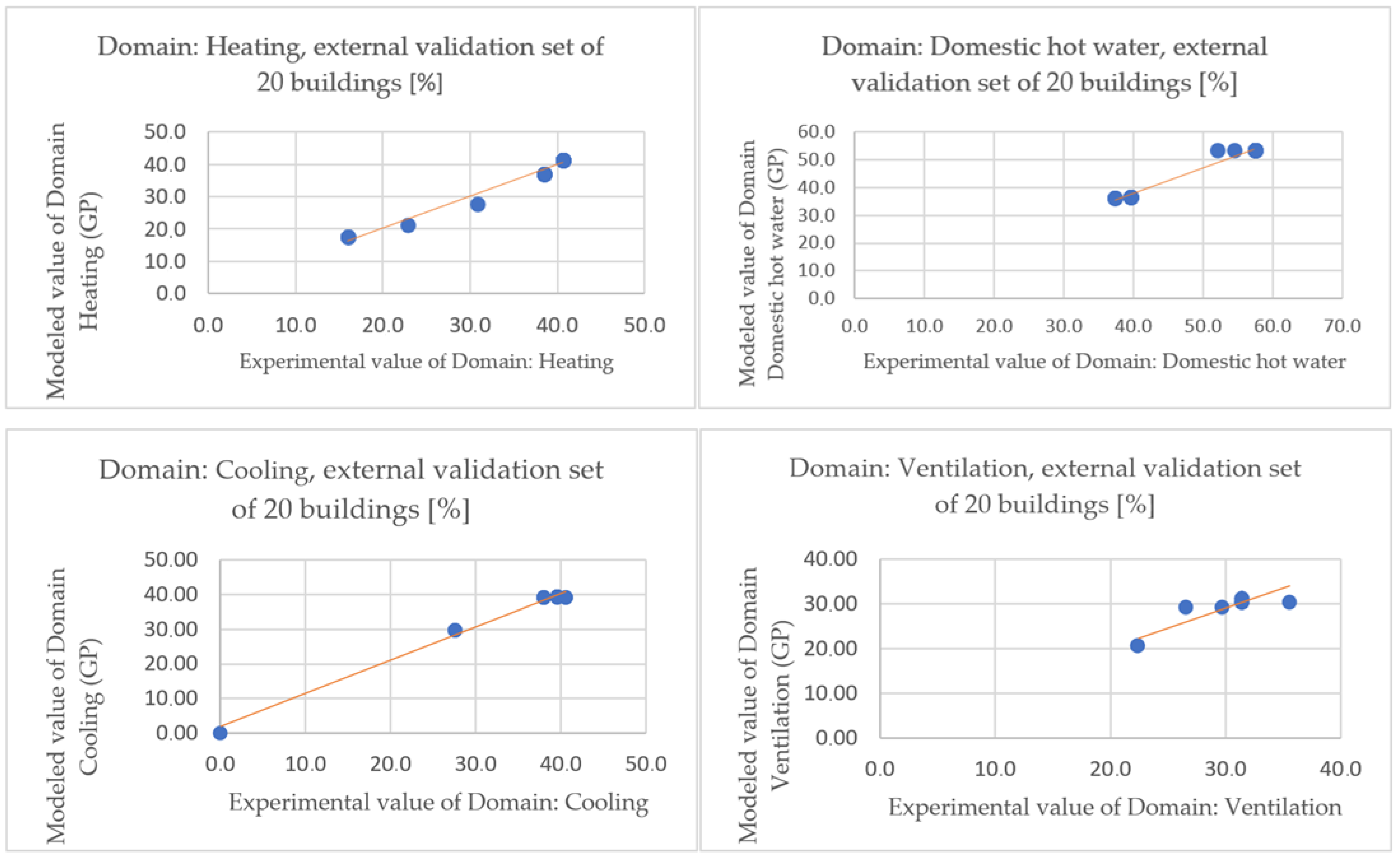
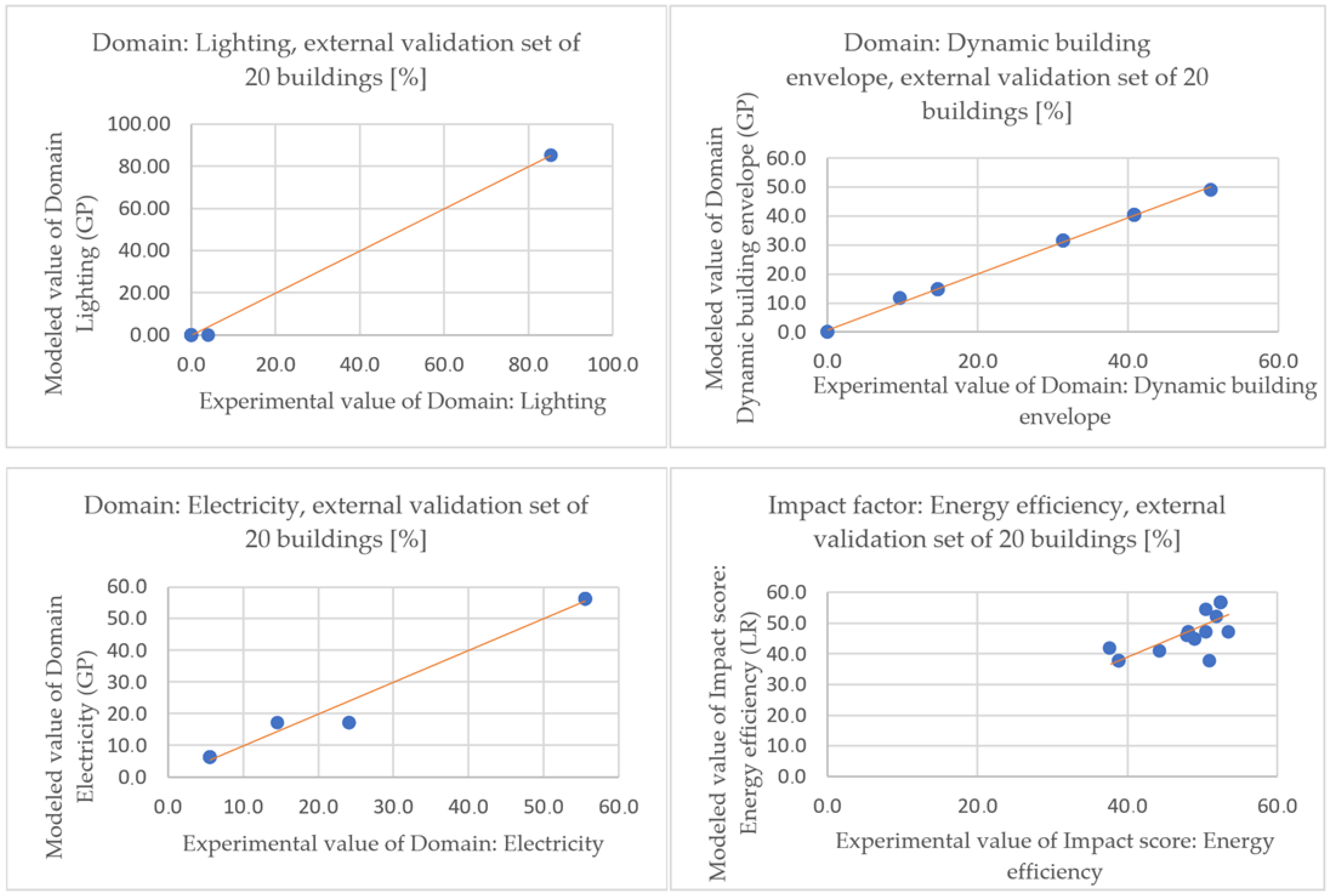
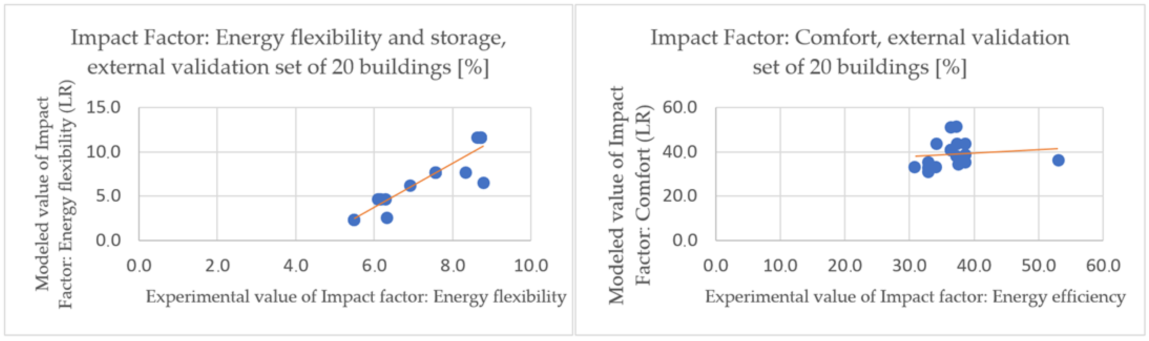
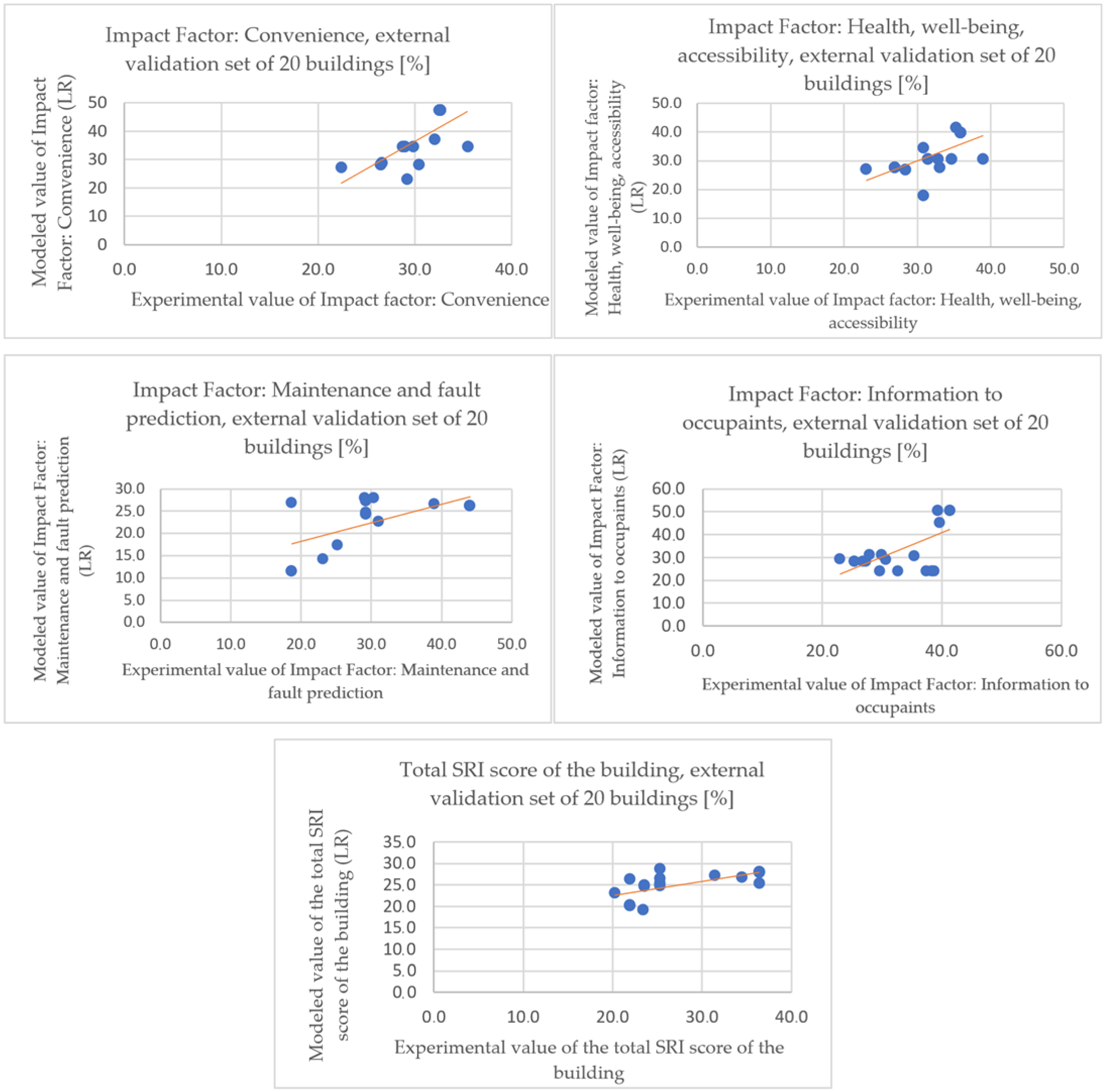
4.3. Validation of the GP + LR Models

A supplementary validation experiment was carried out utilising a fresh, independent dataset consisting of 20 new buildings. The aim of this experiment was to evaluate the generalisability and applicability of the models in real-world conditions. The distribution of the case studies by purpose of use was comparable to that used in the model training phase (presented in Figure 1), ensuring consistency in the sample characteristics. None of these buildings were part of the training or model development process and were assessed using both the official SRI Excel-based calculation tool (as the reference method) and the GP + LR models (as the predictive method). For each building, predictions were generated for Domain-level scores, Impact Factors, and the total SRI score.
The performance of the models was tested with the following five most commonly used statistical metrics [58,59]:
  • Mean absolute error (MAE);
  • Root mean squared error (RMSE);
  • Mean bias error (MBE);
  • Coefficient of determination (R2);
  • Pearson’s correlation coefficient (r).
The results of the experiment are presented in Table 5, and they demonstrate the model’s ability to generalise across unseen data, building typologies, and system configurations.
The graphical results of this validation experiment illustrating the modelled versus experimental values for each Domain, Impact Factor, and the total SRI score are presented in the multi-panel Figure 4 and Figure 5 on the following two pages. The figures provide a visual interpretation of the model’s performance across the 20 tested external buildings. A detailed discussion is provided in Section 5.3. Validation of the Developed Models.

5. Discussion

The presented paper describes the creation of alternative, simplified, and sufficiently precise SRI calculation models based on GP and LR. The methods used in the individual steps are summarised in Table 6.
GP was suitable for Domain modelling, as the inputs were discrete numbers that describe the state of whether a smart service exists in the examined building (0—the observed smart service is absent, 1—the observed service is present, 2—the service cannot be evaluated because the building does not have such a system). By obtaining Domain scores, we were able to use LR to predict the building’s Impact Factors and overall SRI scores.

5.1. Modelling Domains

As is evident from Figure 2, the relative deviation from the experimental Domain scores is relatively low, ranging between 0.92% (the dynamic building envelope Domain) to 2.97% (the cooling Domain), indicating high model accuracy. The small difference shows that the developed models captured the main patterns in the data well and can reproduce the results reliably. The strong agreement between the modelled Domain scores and experimental Domain scores confirms the robustness of the proposed approach, demonstrating its suitability for predictive applications. Nevertheless, the relative deviation from the experimental data for EV charging and monitoring and control Domains is not stated in Figure 2, since the models for these two Domains could not be developed. The details are explained in the paragraphs addressing the limitations and challenges of this study.

5.2. Modelling Impact Factors

The linear regression statistics for modelling the Impact Factors presented in Table 4 demonstrate the generally strong model performance across most Impact Factors, with R2 values ranging from 0.58 to 0.99. The highest explanatory power was observed in the total SRI score (R2 = 0.99), indicating excellent alignment between predicted and reference values at the aggregated level. Most Impact Factors, like energy efficiency (R2 = 0.76), convenience (R2 = 0.81), and comfort (R2 = 0.75) demonstrated high levels of predictive accuracy.
Impact Factors with lower R2 values were observed in health, well-being, and accessibility (R2 = 0.65), maintenance and fault prediction (R2 = 0.72), and information to the occupants (R2 = 0.62). This reduced predictive performance can be attributed to the qualitative and often subjective nature of these categories. Unlike Domains that evaluate clearly defined technical features (e.g., heating or lighting systems), these Impact Factors depend more heavily on user experience, communication features, accessibility standards, and the presence of advanced automation systems, such as BMS or user interaction platforms. In many cases, such features are not implemented or documented across buildings consistently, particularly in the South-East European region, where system standardisation and data availability may be limited. As a result, the training data lack the diversity and clarity needed to build stronger predictive models for these factors. The variability in interpretation or recording of these services during the SRI experimental evaluations may have lowered the power of the model’s ability to capture consistent patterns. These limitations suggest that improved documentation and richer datasets with standardised descriptions of non-technical smart services are essential to enhance model reliability in these more subjective categories.
The lowest R2 value (0.577) was found in the energy flexibility and storage Impact Factor. This Domain primarily evaluates smart hardware and system integrations that support thermal and electrical energy storage, including advanced technologies, such as fourth-generation district heating networks. These solutions are promoted by the SRI methodology actively to support future-ready and low-carbon energy infrastructure. However, these technologies are largely absent in the case study buildings from the South-East European region, which provided the basis for the training dataset. As a result, the model had limited exposure to relevant examples, reducing its ability to explain the variance in this Domain accurately. The relatively low R2 value should, therefore, be interpreted not as a sign of model weakness or overfitting, but rather as a reflection of the sparse data related to this advanced system type in the regional context.
The fluctuations in Impact Factor scores can likewise be attributed to the reality that each Impact Factor is calculated from Domain scores, thereby adding extra intricacy and the likelihood of discrepancies.

5.3. Validation of the Developed Models

As mentioned in Section 4.3, to assess the generalisability of the developed models, the models were tested with a new dataset of 20 case study buildings previously unseen in the training. As evident from Table 5, the statistical performance of the model was strong on the Domain level. The values for R2 were above 0.97 for almost all Domains, except for ventilation (R2 = 0.83). Also, the Pearson correlation coefficients were above 0.90 for nearly all the Domains. These results indicate that the GP and LR models are capable of estimating Domain scores accurately, even when applied to buildings outside of the original training set. Particularly high accuracy was observed in several Domains, such as lighting and the dynamic building envelope, where the correlation reached 1.00, and the error values (MAE and RMSE) were minimal.
At the Impact Factor level, the performance varied more significantly. The R2 values for energy efficiency (R2 = 0.59) and energy flexibility and storage (R2 = 0.84) indicate that the predictive accuracy of these Impact Factors is notably influenced by the specific configurations of heating, cooling, and domestic hot water systems in the evaluated buildings. The variability in system setups and the presence or absence of advanced energy management features likely contributed to the observed differences in R2 values, suggesting that the model’s performance in these categories is closely tied to the particular combinations of these systems.
The lower R2 and Pearson correlation (r) values observed for several Impact Factors, including comfort (R2 = 0.42, r = 0.65), convenience (R2 = 0.54, r = 0.73), health, well-being, and accessibility (R2 = 0.42, r = 0.65), maintenance and fault prediction (R2 = 0.42, r = 0.65), and information to occupants (R2 = 0.39, r = 0.63) are closely tied to the presence of advanced building management systems (BMSs) and automated control functions. The external dataset of 20 buildings included a limited number of buildings equipped with highly advanced BMS functions, such as predictive maintenance and advanced energy monitoring. This likely contributed to the weaker statistical performance for these Impact Factors.
The total SRI score prediction across all buildings yielded an R2 of 0.48 and a Pearson correlation of 0.69, indicating moderate alignment between the predicted and reference values. The mean absolute error of 4.45 and mean bias error of −3.0 suggest that while the model may underpredict slightly on average, the estimates are reasonably close to the official results generated using the SRI Excel tool. These findings confirm that the model has practical applicability in real-world conditions, particularly for Domain-level estimations, while also highlighting areas where further training data and refinement may improve robustness at the Impact Factor and total score level.

5.4. Limitations and Challenges

However, two out of the nine investigated Domains could not be modelled effectively using the method of GP. These two Domains are EV charging and monitoring and control. The primary reason for this limitation was the inconsistent experimental data used to develop the model. Despite utilising a large database of 223 case study buildings, the data exhibited a high degree of randomness, preventing the identification of meaningful patterns. The variability within these datasets was significantly higher than in the other Domains, leading to unstable model predictions. Therefore, no reliable correlation could be established between the input parameters and the expected outcomes. The unpredictability in the data suggests the presence of uncontrolled influences or measurement inconsistencies. In contrast, the remaining seven Domains exhibited structured and consistent data, allowing for high-quality modelling. This limitation could likely be resolved with a larger and more comprehensive dataset.
The absence of the electric vehicle charging and monitoring and control Domains did not impact the modeling of other Domains, as each Domain was treated independently in the model. Inputs for these two Domains were included in the model structure of LR for the Impact Factor calculations (LR model No. 18), suggesting that with a more consistent dataset, they could potentially be modelled effectively in future iterations.

5.5. Scalability and Transferability of the Developed Models Across Europe

A dataset of 223 buildings from the South-East European region was leveraged to generate the GP models for Domains. In the original SRI methodology, there are several regions that the evaluator can choose from (“North Europe”, “West Europe”, “South Europe”, “South-West Europe”, “North-East Europe”, and “South-East Europe”). A similar case study building dataset would have to be prepared if the proposed methods were to be used in another region. Considering this, it must be ensured that the cases are selected in a balanced manner, as this affects the accuracy of the final model. Based on our study, it is clear that the current model reflects the building system configurations common to that region, including typical HVAC control setups. Regional differences in technical systems can influence the SRI outcomes. However, once the model structure and methodology have been defined (as in our case) it becomes relatively easy to train new models for other regions using localised datasets.
The limited applicability of SRI models, for example, in colder regions, was highlighted in one of the first studies [20], as the current SRI framework does not fully reflect some cold-climate-specific technologies, such as advanced district heating systems. The study also pointed out challenges related to the triage process and the comparability of SRI scores across regions. Also, the study [37] noted that regional differences in technical systems can influence the SRI outcomes. These insights further reinforce the need to adapt SRI tools (and models based on them) to local building practices when aiming for EU-wide applicability.

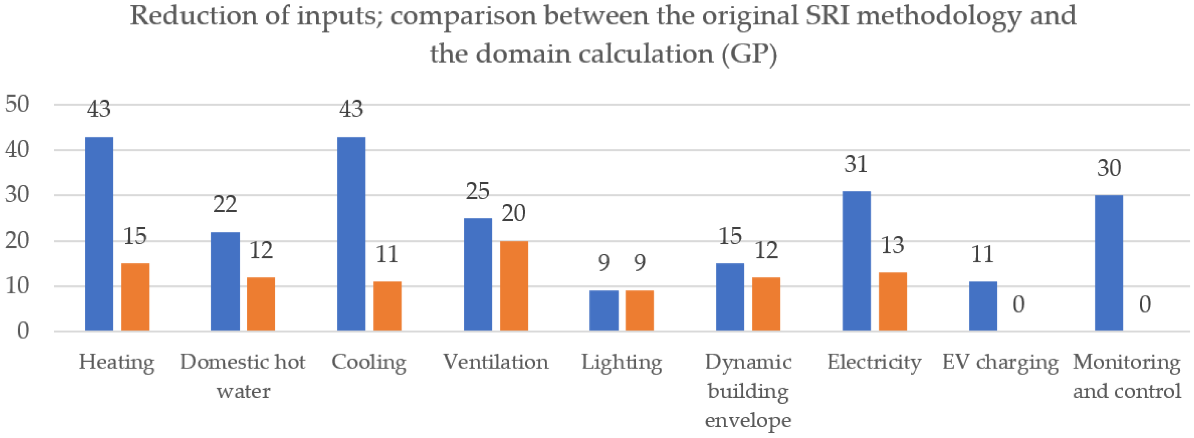
5.6. Reduction in the Needed Inputs for the Calculation

It must be highlighted that, by utilising GP modelling, we were able to reduce the total number of inputs (or organisms in GP models) while still maintaining the adequate accuracy of the models needed to achieve comparable results. The inputs/genes that the GP used in the models are underlined in Appendix A.
Table 7 compares “smart-ready” service levels in the original methodology with the necessary inputs in the GP models for Domain calculation with the % of reduction. The results are presented also graphically in Figure 6.
Noticeably, some inputs appear much more frequently in the Domain calculation models (generated with GP) than others. These inputs have a higher dominance than the rest, which is the by-product of natural selection on which the GP is based. The inputs that appear very often (more than 15 times) in the models for modelling Domains are presented in Table 8. From a practical perspective, these have a high impact on reaching a higher SRI score.

6. Conclusions

The EU must accelerate the execution of the initiatives outlined in the Green Deal. As a result, substantial endeavours are necessary for the decarbonisation of the building inventory. An innovative tool, the Smart Readiness Indicator (SRI), aims to facilitate the implementation of intelligent solutions across various building types.
Our research shows that alternative, simplified, and sufficiently precise SRI calculation models based on GP and LR are possible. The developed models proved to be sufficiently accurate. The relative deviation from the experimental data for Domain scores (modelled with GP) ranged from 0.9% to 2.9%. The coefficient of determination or R2 was 0.75 for most LR models, except for the Impact Factor of “Energy flexibility and storage” (where it was 0.57). The lower R2 value for this Impact Factor is due to the absence of advanced systems, like fourth-generation district heating, in the evaluated case study buildings. These technologies are not common in the South-East European region, resulting in limited training data in our dataset. For the total SRI core the R2 it was 0.98.
To test how well the models work on new data, we carried out an external validation using 20 previously unseen case study buildings. In this way, we checked the performance of the GP + LR approach on buildings that were not part of the model development. On the Domain-level, the predictions performed well, with R2 values between 0.83 and 1.00. For the Impact Factors, the performance was more variable, with R2 values between 0.39 and 0.84. The total SRI score prediction reached R2 = 0.48, with MAE = 4.45 and Pearson’s r = 0.69, which shows that the model can also work in real world conditions.
Our findings suggest that the existing model represents the building system configurations typically present in that area accurately, including conventional HVAC and control arrangements. Variations in technical systems across regions impact SRI results. After establishing the model structure and methodology (as demonstrated in our instance), it becomes fairly straightforward to develop new models for different regions utilising localised datasets. Larger datasets based on consistently audited buildings would improve the reliability and accuracy of SRI predictions by providing the models with more diverse and representative examples across different systems and building types.
To improve consistency and reduce variability, especially in Domains with less structured data, we plan to establish data quality assurance procedures and policies that would guide building evaluations. Cooperation is planned with energy agencies across Europe. With this, we hope to obtain quality data that will be used for further model training. We also aim to integrate the model with digital building twin platforms [36,37], which could support standardised data collection and enable easier data sharing. In Domains where uncertainty remains high, manual review processes (like audits) could be included to avoid misleading outputs. The GP + LR model could be especially useful for portfolio-level screening, early-stage assessments, and decision tools, such as those used by public authorities or real-estate managers.
The GP approach with the additional positive feature has proven that comparable results can be achieved with a significantly smaller number of input variables than in the original SRI methodology. In six out of nine Domains, the reduction was between 20% and 74.42%, while the number of inputs in one Domain (that of lighting) stayed the same.
  • In our case, two out of the nine Domains (electric vehicle charging and monitoring and control) could not be modelled because of inconsistencies in the experimental data. The data exhibited a high degree of randomness, preventing modelling. A different dataset may behave differently. Furthermore, for the initial calculation in a selected EU region, a reference dataset of experimental case study examinations is needed (see Section 2, i.e., the description of the experimental data).
The inputs into the GP, highlighted in Table 8, dominate, and are at the core of the Domains’ score calculation. Therefore, this GP model could also be used as a simulation tool for architects and planners of electrical and mechanical systems, including the smart-ready functions that impact the SRI scores the most.
Our future research will focus on the automation of the evaluation process.

Author Contributions

Conceptualisation, M.B. (Mitja Beras), U.Ž., and M.K.; Methodology: M.B. (Mitja Beras), U.Ž., and M.K. Investigation, M.B. (Mitja Beras); Formal Analysis, M.B. (Mitja Beras); Writing—Original Draft Preparation, M.B. (Mitja Beras); Writing—Review and Editing, M.B. (Mitja Beras), U.Ž., and M.K.; Visualisation, M.B. (Mitja Beras); Validation U.Ž. and M.B. (Mitja Beras); Software, M.K.; Supervision, M.B. (Mitja Beras), M.B. (Miran Brezočnik) and U.Ž. All authors have read and agreed to the published version of the manuscript.

Funding

This research received no external funding.

Data Availability Statement

The data are not publicly available due to business confidentiality.

Acknowledgments

The authors wish to acknowledge the support provided in the experimental part by the company FENIKS PRO d.o.o.

Conflicts of Interest

Authors declare there is no conflict of interest. Authors declare that the research was conducted in the absence of any commercial or financial relationships that could be construed as a potential conflict of interest. The company Feniks pro had no role in the design of the study.

Appendix A

Table A1. Conversion table of variables for the heating Domain.
LabelInput Data or Organisms for the Genetic Model/Service for Smart-Ready Services and Their Functionality Levels from the Original SRI Methodology [12]
HA1
H1A2
H1A3
H1A4
H1A5
No automatic control
Central automatic control (e.g., central thermostat)
Individual room control (e.g., thermostatic valves, or electronic controller)
Individual room control with communication between controllers and BACS
Individual room control with communication and occupancy detection
H1B1
H1B2
H1B3
H1B4

H1C1
H1C2
H1C3
H1D1
H1D2
H1D3
H1D4
H1D5
H1F1
H1F2
H1F3
H1F4
H2A1
H2A2
H2A3

H2B1
H2B2

H2B3

H2B4

H2D1
H2D2
H2D3


H2D4

H2D5


H31
H32

H33
H34

H35


H41
H42
H43
H44
H45
No automatic control
Central automatic control
Advanced central automatic control
Advanced central automatic control with intermittent operation and/or room temperature feedback control
No automatic control
Outside temperature compensated control
Demand-based control
No automatic control
On/off control
Multi-stage control
Variable speed pump control (pump unit (internal) estimations)
Variable speed pump control (external demand signal)
Continuous storage operation
Time-scheduled storage operation
Load prediction-based storage operation
Heat storage capable of flexible control through grid signals (e.g., DSM)
Constant temperature control
Variable temperature control depending on outdoor temperature
Variable temperature control depending on the load (e.g., depending on supply water temperature set point)
On/off control of heat generator
Multi-stage control of heat generator capacity depending on the load or demand (e.g., on/off for several compressors)
Variable control of heat generator capacity depending on the load or demand (e.g., hot gas bypass, inverter frequency control)
Variable control of heat generator capacity depending on the load AND external signals from grid
Priorities only based on running time
Control according to fixed priority list: e.g., based on rated energy efficiency
Control according to dynamic priority list (based on current energy efficiency, carbon emissions and capacity of generators, e.g., solar, geothermal heat, cogeneration plant, fossil fuels)
Control according to dynamic priority list (based on current AND predicted load, energy efficiency, carbon emissions and capacity of generators)
Control according to dynamic priority list (based on current AND predicted load, energy efficiency, carbon emissions, capacity of generators AND external signals from grid)
None
Central or remote reporting of current performance KPIs (e.g., temperatures, submetering energy usage)
Central or remote reporting of current performance KPIs and historical data
Central or remote reporting of performance evaluation including forecasting and/or benchmarking
Central or remote reporting of performance evaluation including forecasting and/or benchmarking; also including predictive management and fault detection
No automatic control
Scheduled operation of heating system
Self-learning optimal control of heating system
Heating system capable of flexible control through grid signals (e.g., DSM)
Optimised control of heating system based on local predictions and grid signals (e.g., through model predictive control)
Table A2. Conversion table of variables for the domestic hot water Domain.
LabelInput Data or Organisms for the Genetic Model/Service for Smart-Ready Services and Their Functionality Levels from the Original SRI Methodology [12]
DHW1A1
DHW1A2
DHW1A3

DHW1A4

DHW1B1
DHW1B2
DHW1B3


DHW1B4
DHW1D1

DHW1D2
DHW1D3

DHW1D4


DHW2B1
DHW2B2
DHW2B3


DHW2B4

DHW2B5


DHW31
DHW32
DHW33
DHW34
DHW35
Automatic control on/off
Automatic control on/off and scheduled charging enable
Automatic control on/off and scheduled charging enable and multi-sensor storage management
Automatic charging control based on the local availability of renewables or information from electricity grid (DR, DSM)
Automatic control on/off
Automatic control on/off and scheduled charging enabled
Automatic on/off control, scheduled charging enabled, and demand-based supply temperature control or multi-sensor storage management
DHW production system capable of automatic charging control based on external signals (e.g., from the district heating grid)
Manually selected control of solar energy or heat generation
Automatic control of solar storage charge (Prio. 1) and supplementary storage charge
Automatic control of solar storage charge (Prio. 1) and supplementary storage charge and demand-oriented supply or multi-sensor storage management
Automatic control of solar storage charge (Prio. 1) and supplementary storage charge, demand-oriented supply, and return temperature control and multi-sensor storage management
Priorities only based on running time
Control according to fixed priority list: e.g., based on rated energy efficiency
Control according to dynamic priority list (based on current energy efficiency, carbon emissions, and capacity of generators, e.g., solar, geothermal heat, cogeneration plant, and fossil fuels)
Control according to dynamic priority list (based on current AND predicted load, energy efficiency, carbon emissions, and capacity of generators)
Control according to dynamic priority list (based on current AND predicted load, energy efficiency, carbon emissions, capacity of generators, AND external signals from grid)
None
Indication of actual values (e.g., temperatures, submetering energy usage)
Actual values and historical data
Performance evaluation, including forecasting and/or benchmarking
Performance evaluation, including forecasting and/or benchmarking; also including predictive management and fault detection
Table A3. Conversion Table of variables for the cooling Domain.
LabelInput Data or Organisms for the Genetic Model/Service for Smart-Ready Services and Their Functionality Levels from the Original SRI Methodology [12]
C1A1
C1A2
C1A3
C1A4

C1A5
C1B1
C1B2
C1B3
C1B4

C1C1
C1C2
C1C3
C1D1
C1D2
C1D3
C1D4
C1D5
C1F1
C1F2

C1F3

C1G1
C1G2
C1G3
C1G4
C2A1
C2A2

C2A3

C2A4

C2B1
C2B2

C2B3

C2B4

C2B5

C31
C32

C33
C34

C35


C41
C42
C43
C44
C45
No automatic control
Central automatic control
Individual room control
Individual room control with communication between controllers and to BACS
Individual room control with communication and occupancy detection
No automatic control
Central automatic control
Advanced central automatic control
Advanced central automatic control with intermittent operation and/or room temperature feedback control
Constant temperature control
Outside temperature compensated control
Demand based control
No automatic control
On off control
Multi-stage control
Variable speed pump control (pump unit (internal) estimations)
Variable speed pump control (external demand signal)
No interlock
Partial interlock (minimising risk of simultaneous heating and cooling e.g., by sliding setpoints)
Total interlock (control system ensures no simultaneous heating and cooling can take place)
Continuous storage operation
Time-scheduled storage operation
Load prediction-based storage operation
Cold storage capable of flexible control through grid signals (e.g., DSM)
On/off control of cooling production
Multi-stage control of cooling production capacity depending on the load or demand (e.g., on/off for several compressors)
Variable control of cooling production capacity depending on the load or demand (e.g., hot gas bypass, inverter frequency control)
Variable control of cooling production capacity depending on the load AND external signals from grid
Priorities only based on running times
Fixed sequencing based on loads only, e.g., depending on the generator’s characteristics, such as absorption chiller vs. centrifugal chiller
Dynamic priorities based on generator efficiency and characteristics (e.g., availability of free cooling)
Load prediction-based sequencing: the sequence is based on e.g., COP and the available power of a device and the predicted required power
Sequencing based on a dynamic priority list, including external signals from grid
None
Central or remote reporting of current performance KPIs (e.g., temperatures, submetering energy usage)
Central or remote reporting of current performance KPIs and historical data
Central or remote reporting of performance evaluation, including forecasting and/or benchmarking
Central or remote reporting of performance evaluation, including forecasting and/or benchmarking; also including predictive management and fault detection
No automatic control
Scheduled operation of cooling system
Self-learning optimal control of cooling system
Cooling system capable of flexible control through grid signals (e.g., DSM)
Optimised control of cooling system based on local predictions and grid signals (e.g., through model predictive control)
Table A4. Conversion Table of variables for variables for the ventilation Domain.
LabelInput Data or Organisms for the Genetic Model/Service for Smart-Ready Services and Their Functionality Levels from the Original SRI Methodology [12]
V1A1
V1A2
V1A3
V1A4

V1A5

V1C1

V1C2

V1C3
V1C4

V1C5


V2C1
V2C2
V2C3

V2D1
V2D2


V2D3
V2D4


V31
V32
V33

V34


V61
V62
V63
V64
No ventilation system or manual control
Clock control
Occupancy detection control
Central demand control based on air quality sensors (CO2, VOC, humidity, etc.)
Local demand control based on air quality sensors (CO2, VOC, etc.) with local flow to/from the zone regulated by dampers
No automatic control: continuously supplies air flow for a maximum load of all rooms
On/off time control: continuously supplies air flow for a maximum load of all rooms during nominal occupancy time
Multi-stage control: to reduce the auxiliary energy demand of the fan
Automatic flow or pressure control without pressure reset: load-dependent supply of air flow to meet the demands of all connected rooms
Automatic flow or pressure control with pressure reset: load-dependent supply of air flow for the demand of all connected rooms (for variable air volume systems with VFD)
Without overheating control
Modulate or bypass heat recovery based on sensors in air exhaust
Modulate or bypass heat recovery based on multiple room temperature sensors or predictive control
No automatic control
“Constant setpoint: A control loop enables to control the supply air
temperature, the setpoint is constant and can only be modified by a manual
action”
Variable set point with outdoor temperature compensation
Variable set point with load-dependent compensation. A control loop enables the system to control the supply air temperature. The setpoint is defined as a function of the loads in the room
No automatic control
Night cooling
“Free cooling: air flows modulated during all periods of time to minimize the amount of mechanical cooling”
“H,x- directed control: The amount of outside air and recirculation air are modulated during all periods of time to minimize the amount of mechanical cooling. Calculation is performed on the basis of temperatures and humidity
(enthalpy).”
None
Air quality sensors (e.g., CO2) and real-time autonomous monitoring
Real time monitoring and historical information of IAQ available to occupants
Real time monitoring and historical information of IAQ available to occupants + warnings about maintenance needs or occupant actions (e.g., window opening)
Table A5. Conversion Table of variables for the lighting Domain.
LabelInput Data or Organisms for the Genetic Model/Service for Smart-Ready Services and Their Functionality Levels from the Original SRI Methodology [12]
L1A1
L1A2
L1A3
L1A4
L21
L22
L23
L24
L25
Manual on/off switch
Manual on/off switch + additional sweeping extinction signal
Automatic detection (auto on/dimmed or auto off)
Automatic detection (manual on/dimmed or auto off)
Manual (central)
Manual (per room/zone)
Automatic switching
Automatic dimming
“Automatic dimming including scene-based light control (during time intervals, dynamic and adapted lighting scenes are set, for example, in terms of
illuminance level, different correlated colour temperature (CCT) and the possibility to change the light distribution within the space according to e. g. design, human needs, visual tasks)”
Table A6. Conversion Table of variables for the dynamic building envelope Domain.
LabelInput Data or Organisms for the Genetic Model/Service for Smart-Ready Services and Their Functionality Levels from the Original SRI Methodology [12]
DE11
DE12
DE13
DE14
DE15
DE21
DE22
DE23

DE24

DE41
DE42
DE43
DE44

DE45
No sun shading or only manual operation
Motorised operation with manual control
Motorised operation with automatic control based on sensor data
Combined light/blind/HVAC control
Predictive blind control (e.g., based on weather forecasts)
Manual operation or only fixed windows
Open/closed detection to shut down heating or cooling systems
Level 1 + automated mechanical window opening based on room sensor data
Level 2 + centralised coordination of operable windows, e.g., to control free natural night cooling
No reporting
Position of each product and fault detection
Position of each product, fault detection, and predictive maintenance
Position of each product, fault detection, predictive maintenance, and real-time sensor data (wind, lux, temperature, etc.)
Position of each product, fault detection, predictive maintenance, and real-time and historical sensor data (wind, lux, temperature, etc.)
Table A7. Conversion Table of variables for the electricity Domain.
LabelInput data or organisms for the genetic model/service for smart-ready services and their functionality levels from the original SRI methodology [12]
EL21
EL22
EL23
EL24
EL25

EL31
EL32
EL33

EL34

EL35


EL41
EL42
EL43

EL44

EL51

EL52

EL53


EL81
EL82

EL83
EL84


EL111
EL112
EL113
EL114
EL115

EL121
EL122
EL123
EL124
EL125
None
Current generation data available
Actual values and historical data
Performance evaluation including forecasting and/or benchmarking
Performance evaluation including forecasting and/or benchmarking; also including predictive management and fault detection
None
On-site storage of electricity (e.g., electric battery)
On-site storage of energy (e.g., electric battery or thermal storage) with a controller based on grid signals
On-site storage of energy (e.g., electric battery or thermal storage) with a controller optimising the use of locally generated electricity
On-site storage of energy (e.g., electric battery or thermal storage) with a controller optimising the use of locally generated electricity and the possibility to feed back into the grid
None
Scheduling electricity consumption (plug loads, white goods, etc.)
Automated management of local electricity consumption based on current renewable energy availability
Automated management of local electricity consumption based on current and predicted energy needs and renewable energy availability
CHP control based on scheduled runtime management and/or current heat energy demand
CHP runtime control influenced by the fluctuating availability of RES; overproduction will be fed into the grid
CHP runtime control influenced by the fluctuating availability of RES and grid signals; dynamic charging and runtime control to optimise the self-consumption of renewables
None
Automated management of (building-level) electricity consumption based on grid signals
Automated management of (building-level) electricity consumption and electricity supply to neighbouring buildings (microgrid) or grid
Automated management of (building-level) electricity consumption and supply, with potential to continue limited off-grid operation (island mode)
None
Current state of charge (SOC) data available
Actual values and historical data
Performance evaluation, including forecasting and/or benchmarking
Performance evaluation, including forecasting and/or benchmarking; also including predictive management and fault detection
None
Reporting on current electricity consumption at the building level
Real-time feedback or benchmarking at the building level
Real-time feedback or benchmarking at the appliance level
Real-time feedback or benchmarking at the appliance level with automated personalised recommendations
Table A8. Conversion Table of variables for the EV charging Domain.
LabelInput Data or Organisms for the Genetic Model/Service for Smart-Ready Services and their Functionality Levels from the Original SRI Methodology [12]
EV151
EV152
EV153
EV154
EV155
EV161
EV162

EV163

EV171
EV172
EV173
Not present
Ducting (or simple power plug) available
0–9% of parking spaces has recharging points
10–50% or parking spaces has recharging point
>50% of parking spaces has recharging point
Not present (uncontrolled charging)
1-way controlled charging (e.g., including desired departure time and grid signals for optimisation)
2-way controlled charging (e.g., including desired departure time and grid signals for optimisation)
No information available
Reporting information on EV charging status to occupants
Reporting information on EV charging status to occupants AND automatic identification and authorisation of the driver to the charging station (ISO 15118 compliant)
Table A9. Conversion Table of variables for the monitoring and control Domain.
LabelInput Data or Organisms for the Genetic Model/Service for Smart-Ready Services and Their Functionality Levels from the Original SRI Methodology [12]
MC31
MC32

MC33
MC34

MC41
MC42
MC43
MC44

MC91
MC92

MC93

MC131
MC132

MC133

MC134

MC251

MC252

MC253
MC281
MC282
MC283

MC291
MC292

MC293
MC294
MC295
MC301
MC302
MC303
MC304
Manual setting
Runtime setting of heating and cooling plants following a predefined time schedule
Heating and cooling plant on/off control based on building loads
Heating and cooling plant on/off control based on predictive control or grid signals
No central indication of detected faults and alarms
With central indication of detected faults and alarms for at least two relevant TBS
With central indication of detected faults and alarms for all relevant TBS
With central indication of detected faults and alarms for all relevant TBS, including diagnosing functions
None
Occupancy detection for individual functions, e.g., lighting
Centralised occupant detection which feeds into several TBS, such as lighting and heating
None
Central or remote reporting of real-time energy use per energy carrier
Central or remote reporting of real-time energy use per energy carrier, combining TBS of at least two Domains in one interface
Central or remote reporting of real-time energy use per energy carrier, combining TBS of all main Domains in one interface
None—No harmonisation between grid and TBS; building is operated independently from the grid load
Demand-side management possible for (some) individual TBS, but not coordinated over various Domains
Coordinated demand side management of multiple TBS
None
Reporting information on current DSM status, including managed energy flows
Reporting information on current historical and predicted DSM status, including managed energy flows
No DSM control
DSM control without the possibility to override this control by the building user (occupant or facility manager)
Manual override and reactivation of DSM control by the building user
Scheduled override of DSM control (and reactivation) by the building user
Scheduled override of DSM control and reactivation with optimised control
None
Single platform that allows manual control of multiple TBS
Single platform that allows automated control and coordination between TBS
Single platform that allows automated control and coordination between TBS + optimisation of energy flow based on occupancy, weather, and grid signals

Appendix B

The equation form of the genetic programming model for heating is as follows:
D o m a i n   H e a t i n g =   H 33 H 2 D 5 · H 2 B 3 H 1 C 2 + H 31 7.16973 5.81691 + H 2 D 1 · H 33 H 2 D 2 · H 2 B 3 H 1 C 2 + H 31 7.16973 5.81691 + H 2 D 1 · 7.16973 H 33 H 1 B 2 · H 44 H 2 D 5 · H 2 B 3 H 1 C 2 + H 31 H 33 + H 1 C 2 + H 2 B 3 H 2 D 5 · H 33 + H 1 A 5 + H 2 B 1 · H 1 A 4 · H 33 + H 1 A 5 + H 2 B 1 H 1 A 5 + H 1 A 4 · H 31 H 33 9.66955 H 2 D 5 · H 2 B 3 H 1 C 2 H 1 C 2 H 2 D 2 H 2 D 1 · H 2 D 2 + 9.66955 H 2 D 5 · H 2 B 3 · H 1 C 2 + H 31 H 2 D 2 H 2 D 1 · H 2 B 1 · H 2 D 2 · 5.46992
The equation form of the genetic programming model for domestic hot water is as follows:
D o m a i n   D o m e s t i c   h o t   w a t e r = D H W 1 D 1 · D H W 2 B 5 D H W 1 A 4 + D H W 1 B 1 · D H W 2 B 5 D H W 1 A 4 + 3.1451 D H W 1 B 1 · D H W 1 D 3 3.14511 D H W 1 D 1 · D H W 1 A 2 D H W 1 B 3 D H W 2 B 1 + 9.18609 D H W 32 · D H W 1 D 3 3.14511 D H W 1 B 3 D H W 2 B 1 + 9.18609 D H W 32 · D H W 1 D 1 · D H W 1 A 2 D H W 1 D 1 D H W 1 A 4 D H W 31 + D H W 2 B 2 D H W 34 + D H W 2 B 1 D H W 1 D 3 D H W 1 A 4 · D H W 1 B 1 · D H W 31 + D H W 34 3.14511 D H W 1 D 3 · D H W 1 A 4 · D H W 1 B 1 · D H W 31 + D H W 2 B 1 · D H W 2 B 5 D H W 2 B 5 D H W 1 A 4 · D H W 1 B 1 · D H W 31 D H W 2 B 1 + 9.18609 D H W 2 B 5 · 3.21647
The equation form of the genetic programming model for cooling is as follows:
D o m a i n   c o o l i n g = C 1 B 2 + C 2 A 1 7.66353 C 1 A 4 · C 1 A 4 · C 1 F 1 · C 34 · C 1 F 1 C 43 C 1 A 4 · 7.66353 + C 1 F 1 C 43 · C 1 F 3 C 1 D 3 · C 1 D 1 · C 2 A 1 7.66353 + C 43 C 1 F 1 C 1 F 3 C 43 C 2 A 1 C 1 F 1 · C 1 D 3 · C 1 D 5 + C 1 A 4 · C 2 A 1 7.66353 + C 43 + C 1 F 1 · C 34 · 7.66353 C 43 + C 43 C 1 F 1 C 43 C 1 F 1 C 1 F 3 + C 43 C 2 A 1 C 1 F 1 + C 43 · C 34 · 7.66353 C 1 F 1 C 43 C 1 F 1 C 1 F 3 C 1 D 3 + C 1 D 5 + C 1 F 1 7.66353 + C 43 C 1 F 1 7.66353 + C 43 · C 34 C 1 F 1 C 43 · C 1 A 4 · 7.66353 + C 43 + C 43 · C 34 C 1 F 1 C 43 · C 1 A 4 · 7.66353 + C 43 + C 43 · C 43 · C 1 F 3 C 1 D 3 + C 1 D 5 · C 1 D 5 + C 1 F 1 · C 34 7.663553
The equation form of the genetic programming model for ventilation is as follows:
D o m a i n   V e n t i l a t i o n = 8.4716 V 31 5.25128 V 2 C 2 · V 1 C 5 V 62 + V 1 C 3 + V 1 A 3 V 62 · V 33 · V 64 84716 + V 64 · V 33 V 31 + V 2 C 2 · V 1 C 5 · V 2 D 2 · V 1 C 3 5.25128 V 1 C 1 V 1 A 2 + V 61 + V 1 C 3 + V 2 C 2 · V 1 C 5 · V 2 D 2 · V 1 C 3 + V 2 C 3 ÷ V 1 C 2 V 61 × 8.4716 V 31 8.4716 V 61 + V 1 C 3 + V 2 C 3 V 1 C 2 V 1 C 2 V 2 C 2 · V 1 C 5 · V 2 D 2 · 5.25128 V 2 D 2 · V 1 C 3 5.25128 V 1 C 2 · V 1 A 5 + V 2 D 3 8.4716 8.4716 V 31 5.25128 V 2 C 2 · V 1 C 5 · V 2 D 2 V 1 C 3 + V 1 A 3 V 62 5.25128 V 64 · V 1 C 1 ÷ V 1 A 2 V 1 A 2 + 8.4716 V 2 C 3 V 1 C 2 V 1 C 2 V 2 C 2 · V 1 C 5 · V 2 D 2 · V 1 C 3 5.25128 · V 62 · V 33 · V 1 A 5 V 2 C 1 V 2 D 1 + V 1 A 2 6.96117 · V 2 D 1 V 2 D 2 V 1 C 4
The equation form of the genetic programming model for lighting is as follows:
D o m a i n   L i g h t i n g = L 25 L 1 A 3 L 21 + L 23 + L 23 + L 1 A 3 L 1 A 1 · 3.27069 · L 25 L 1 A 4 L 24 L 22 · L 1 A 1 × L 25 L 22 L 23 + L 23 + L 22 0.160899 · L 25 L 1 A 3 · L 1 A 1 L 24 + L 1 A 4 + L 21 L 23 + L 23 + L 22 · 0.160899 · L 23 + L 1 A 3 L 25 L 1 A 3 · L 1 A 1 L 24 L 1 A 4 + L 1 A 4 + L 1 A 2 + L 22 L 22 + 3.27069 · L 24 L 1 A 4 + L 1 A 3 · L 1 A 3 L 1 A 1 + L 23 + L 1 A 3 L 22 · L 1 A 2 × L 22 L 24 + L 24 L 1 A 4 + L 1 A 4 + L 1 A 2 ÷ L 23 + L 22 L 1 A 3
The equation form of the genetic programming model for the dynamic building envelope (DBE) is as follows:
D o m a i n   D y n a m i c   b u i l d i n g   e n v e l o p e = D E 41 5.87984 D E 11 · D E 22 · D E 44 + D E 44 D E 15 + D E 42 D E 44 + D E 22 · D E 11 D E 24 · D E 44 + D E 12 + D E 23 + D E 42 D E 44 + D E 22 · D E 11 D E 42 D E 13 + D E 22 D E 13 + D E 42 D E 13 + D E 22 D E 13 + D E 42 D E 44 + D E 22 · D E 11 D E 24 · D E 11 D E 42 D E 22 D E 11 D E 24 · D E 14 + D E 13 + D E 22 D E 13 + D E 43 D E 12 · D E 22 · D E 11 D E 22 D E 22 D E 13 · D E 44 + D E 22 · D E 14 + D E 42 D E 13 + D E 22 D E 13 + D E 42 D E 13 + D E 22 D E 13 + D E 42 D E 44 + D E 22 · D E 11 D E 24 · D E 11 D E 42 D E 22 D E 11 D E 24 D E 13 + D E 22 D E 42 D E 42
The equation form of the genetic programming model for electricity is as follows:
D o m a i n   E l e c t r i c i t y = E L 35 E L 124 E L 125 · E L 122 7.29756 E L 82 E L 31 E L 124 E L 124 7.29756 E L 82 E L 31 E L 114 E L 124 E L 124 · E L 51 E L 124 E L 125 · 7.29756 E L 82 E L 31 E L 124 E L 122 · E L 122 · 7.29756 E L 125 E L 82 E L 31 7.29756 E L 82 E L 31 E L 125 8.69097       E L 81 E L 122 · E L 34 + E L 122 · E L 41 E L 82 · E L 35 E L 33 E L 124 · E L 51 E L 124 E L 125 · 7.29756 E L 82 E L 31 E L 112

References

  1. European Parliament and of the Council. Regulation (EU) 2018/1999 of the European Parliament and of the Council of 11 December 2018 on the Governance of the Energy Union and Climate Action, Amending Regulations (EC) No 663/2009 and (EC) No 715/2009 of the European Parliament and of the Council; European Parliament and of the Council: Strasbourg, France, 2018; Volume 2018, p. 77. [Google Scholar]
  2. IEA. Perspectives for Clean Energy Transition. The Critical Role of Buildings; International Energy Agency: Paris, France, 2019; p. 117. [Google Scholar]
  3. Commission Recommendation (EU). 2019/786 of 8 May 2019 on the renovation of buildings (Notified Under Document Number C(2019) 3352) (Text with EEA relevance). Off. J. Eur. Union 2019, 2030, 34–79. [Google Scholar]
  4. The European Parliament and the Council of the European Union and of the E. Union. Directive (EU). 2024/1275 of the European parlament and of the council (24 April 2024) on the Energy performance of buildings. Off. J. Eur. Union 2024, 1275, 1–68. [Google Scholar]
  5. European Parliament and of the Council. DIRECTIVE (EU). 2018/844 of the European Parliament and of the Council of 30 May 2018 Amending Directive 2010/31/EU on the energy performance of buildings and Directive 2012/27/EU on the Energy Performance of Buildings (EPBD). Off. J. Eur. Union 2018, 2018, 75–91. [Google Scholar]
  6. Verbeke, S.; Aerts, D.; Reynders, G.; Ma, Y.; Waide, P. Final Report on the Technical Support to the Development of a Smart Readiness Indicator for Buildings; Shorter Version; European Commission: Brussels, Belgium, 2020. [Google Scholar]
  7. Van Thillo, L.; Verbeke, S.; Audenaert, A. The potential of building automation and control systems to lower the energy demand in residential buildings: A review of their performance and influencing parameters. Renew. Sustain. Energy Rev. 2022, 158, 112099. [Google Scholar] [CrossRef]
  8. Domingues, P.; Carreira, P.; Vieira, R.; Kastner, W. Building automation systems: Concepts and technology review. Comput. Stand. Interfaces 2016, 45, 1–12. [Google Scholar] [CrossRef]
  9. Fejr, M. Smart Readiness Indicator and Indoor Environmental Quality: Two Case Studies in Italy and Portugal. Ph.D. Thesis, Politecnico di Torino, Torino, Italy, 2019. [Google Scholar]
  10. Surmeli-Anac, N.; Hermelink, A.H. The Smart Readiness Indicator: A Potential, Forward-Looking Energy Performance Certificate Complement? ECOFYS, A Naigant Co., no. May, 2018. Available online: https://www.researchgate.net/publication/327282871_The_Smart_Readiness_Indicator_A_potential_forward-looking_Energy_Performance_Certificate_complement (accessed on 8 May 2025).
  11. Verbeke, S.; Aerts, D.; Reynders, G.; Ma, Y.; Waide, P. Final Report on the Technical Support to the Development of a Smart Readiness Indicator for Buildings; European Commission: Brussels, Belgium, 2020. [Google Scholar]
  12. RS Ministry of Economic Development and Technology, SRIP SMART CITIES AND COMMUNITIES, Action Plan. 2020, pp. 1–102. Available online: https://pmis-arhiv.ijs.si/wp-content/uploads/2020/04/AN_SRIP_PMiS_2020_2022_3FAZA_EPM.pdf (accessed on 8 May 2025).
  13. Pinto, M.C. Towards Smart Buildings: Is the Smart Readiness Indicator an Effective Tool? Ph.D. Thesis, Politecnico di Torino, Torino, Italy, 2020. [Google Scholar]
  14. Taranu, V.; Zuhaib, S. Smart Readiness Indicator Introductory Report. 2021. Available online: https://x-tendo.eu/wp-content/uploads/2020/01/x-tendo-F1.pdf (accessed on 8 May 2025).
  15. EU. The Energy Performance of Buildings Directive; EU: Geneva, Switzerland, 2024; Volume 1275, pp. 1–68. [Google Scholar]
  16. Fotopoulou, M.; Tsekouras, G.J.; Vlachos, A.; Rakopoulos, D.; Chatzigeorgiou, I.M.; Kanellos, F.D.; Kontargyri, V. Day Ahead Operation Cost Optimization for Energy Communities. Energies 2025, 18, 1101. [Google Scholar] [CrossRef]
  17. Omar, O. Intelligent building, definitions, factors and evaluation criteria of selection. Alexandria Eng. J. 2018, 57, 2903–2910. [Google Scholar] [CrossRef]
  18. Märzinger, T.; Österreicher, D. Supporting the smart readiness indicator-A methodology to integrate a quantitative assessment of the load shifting potential of smart buildings. Energies 2019, 12, 1955. [Google Scholar] [CrossRef]
  19. Janhunen, E.; Pulkka, L.; Säynäjoki, A.; Junnila, S. Applicability of the smart readiness indicator for cold climate countries. Buildings 2019, 9, 102. [Google Scholar] [CrossRef]
  20. Markoska, E.; Jakica, N.; Lazarova-Molnar, S.; Kragh, M.K. Assessment of Building Intelligence Requirements for Real Time Performance Testing in Smart Buildings. In Proceedings of the 2019 4th International Conference on Smart and Sustainable Technologies, Split, Croatia, 18–21 June 2019. [Google Scholar]
  21. Li, H.; Hong, T.; Lee, S.H.; Sofos, M. System-level key performance indicators for building performance evaluation. Energy Build. 2020, 209, 109703. [Google Scholar] [CrossRef]
  22. Dell’Isola, M.; Ficco, G.; Canale, L.; Palella, B.I.; Puglisi, G. An IoT Integrated Tool to Enhance User Awareness on Energy Consumption in Residential Buildings. Atmosphere 2019, 10, 743. [Google Scholar] [CrossRef]
  23. Ramezani, B.; da Silva, M.G.; Simões, N. Application of smart readiness indicator for Mediterranean buildings in retrofitting actions. Energy Build. 2021, 249, 111173. [Google Scholar] [CrossRef]
  24. Vigna, I.; Pernetti, R.; Pernigotto, G.; Gasparella, A. Analysis of the Building Smart Readiness Indicator Calculation: A Comparative Case-Study with Two Panels of Experts. Energies 2020, 13, 2796. [Google Scholar] [CrossRef]
  25. Becchio, C.; Corgnati, S.P.; Crespi, G.; Pinto, M.C.; Viazzo, S. Exploitation of dynamic simulation to investigate the effectiveness of the Smart Readiness Indicator: Application to the Energy Center building of Turin. Sci. Technol. Built Environ. 2021, 27, 1127–1143. [Google Scholar] [CrossRef]
  26. Horák, O.; Kabele, K. Testing of pilot buildings by the SRI method. Vytap. Vetr. Instal. 2019, 28, 331–334. [Google Scholar]
  27. Fokaides, P.A.; Panteli, C.; Panayidou, A. How are the smart readiness indicators expected to affect the energy performance of buildings: First evidence and perspectives. Sustainability 2020, 12, 9496. [Google Scholar] [CrossRef]
  28. Paydar, M.A.; Robertson, C.; Burman, E.; Mumovic, D. A comparison between the impact of dynamic envelope control strategies on the buildings’ smart readiness indicator and modelled performance. Build. Serv. Eng. Res. Technol. 2024, 46, 229–250. [Google Scholar] [CrossRef]
  29. Garzia, F.; Pernigotto, G.; Menegon, D.; Finozzi, L.; Klammsteiner, U.; Gasparella, A. Assessment of the potential correlation between Smart Readiness Indicator and energy performance in a dataset of buildings in South Tyrol. Energy Build. 2024, 321, 114623. [Google Scholar] [CrossRef]
  30. Siddique, M.T.; Koukaras, P.; Ioannidis, D.; Tjortjis, C. A Methodology Integrating the Quantitative Assessment of Energy Efficient Operation and Occupant Needs into the Smart Readiness Indicator. Energies 2023, 16, 7007. [Google Scholar] [CrossRef]
  31. Al Dakheel, J.; Del Pero, C.; Leonforte, F.; Aste, N.; El Mankibi, M. Assessing the performance of smart buildings and smart retrofit interventions through key performance indicators: Defining minimum performance thresholds. Energy Build. 2024, 325, 114988. [Google Scholar] [CrossRef]
  32. Canale, L.; Bongiorno, S.; De Monaco, M.; Di Pietra, B.; La Notte, L.; Badan, N.; Ficco, G.; Puglisi, G.; Dell’Isola, M. Preliminary results of the deployment of the Smart Readiness Indicator in Italy. J. Phys. Conf. Ser. 2024, 2893, 012024. [Google Scholar] [CrossRef]
  33. EN 16247-2:2014; Energy Audits—Part 2: Buildings. European Committee for Standardization (CEN): Brussels, Belgium, 2021. Available online: https://standards.iteh.ai/catalog/standards/cen/3fbb3fd5-0106-42d0-8b9f-cb546db8465a/en-16247-1-2022?srsltid=AfmBOoq_n2Uxg66JUz7iq8iTJcfWKxTdgXzpaNQlzCywmZIM3t9RaO7s (accessed on 8 May 2025).
  34. Martinez, L.; Klitou, T.; Olschewski, D.; Melero, P.C.; Fokaides, P.A. Advancing building intelligence: Developing and implementing standardized Smart Readiness Indicator (SRI) on-site audit procedure. Energy 2025, 316, 134538. [Google Scholar] [CrossRef]
  35. Chatzikonstantinidis, K.; Giama, E.; Fokaides, P.A.; Papadopoulos, A.M. Smart Readiness Indicator (SRI) as a Decision-Making Tool for Low Carbon Buildings. Energies 2024, 17, 1406. [Google Scholar] [CrossRef]
  36. Yang, B.; Lv, Z.; Wang, F. Digital Twins for Intelligent Green Buildings. Buildings 2022, 12, 6. [Google Scholar] [CrossRef]
  37. EN ISO 52120-1:2022; Energy Performance of Buildings–Contribution of Building Automation and Control Systems—Part 1: General Framework and Procedures. European Committee for Standardization (CEN)/International Organization for Standardization (ISO): Brussels, Belgium, 2021. Available online: https://www.iso.org/standard/65883.html (accessed on 8 May 2025).
  38. Walczyk, G.; Ożadowicz, A. Moving Forward in Effective Deployment of the Smart Readiness Indicator and the ISO 52120 Standard to Improve Energy Performance with Building Automation and Control Systems. Energies 2025, 18, 1241. [Google Scholar] [CrossRef]
  39. Commission, E. A Renovation Wave for Europe. COM (2020) 662 final-greening our buildings, creating jobs, improving lives. J. GEEJ 2020, 7, 662. [Google Scholar]
  40. European Commission. European Green Deal Investment Plan; European Commission: Geneva, Switzerland, 2019; No. 35; pp. 44–67. [Google Scholar]
  41. Poli, R.; Langdon, W.B.; McPhee, N.F. A Field Guide to Genetic Programing; Lulu Enterprises: London, UK, 2008. [Google Scholar]
  42. Koza, J.R.; Keane, M.A.; Streeter, M.J.; Mydlowec, W.; Yu, J.; Lanza, G. Genetic Programming IV; Springer: Berlin, Germany, 2005. [Google Scholar]
  43. Górski, A.; Ogorzałek, M. Adaptive iterative improvement GP-based methodology for HW/SW co-synthesis of embedded systems. In Proceedings of the 7th International Joint Conference on Pervasive and Embedded Computing and Communication Systems (PECCS 2017), Madrid, Spain, 24–26 July 2017; pp. 56–59. [Google Scholar]
  44. Ratajczak, J.; Siegele, D.; Niederwieser, E. Maximizing Energy Efficiency and Daylight Performance in Office Buildings in BIM through RBFOpt Model-Based Optimization: The GENIUS Project. Buildings 2023, 13, 1790. [Google Scholar] [CrossRef]
  45. Ayoobi, A.W.; Inceoğlu, M. Developing an Optimized Energy-Efficient Sustainable Building Design Model in an Arid and Semi-Arid Region: A Genetic Algorithm Approach. Energies 2024, 17, 6095. [Google Scholar] [CrossRef]
  46. Farzaneh, H.; Malehmirchegini, L.; Bejan, A.; Afolabi, T.; Mulumba, A.; Daka, P.P. Artificial intelligence evolution in smart buildings for energy efficiency. Appl. Sci. 2021, 11, 763. [Google Scholar] [CrossRef]
  47. Sharma, J.; Shankar Singhal, R. Genetic Algorithm and Hybrid Genetic Algorithm for Space Allocation Problems—A Review. Int. J. Comput. Appl. 2014, 95, 33–37. [Google Scholar] [CrossRef]
  48. Di Filippo, A.; Lombardi, M.; Marongiu, F.; Lorusso, A.; Santaniello, D. Generative design for project optimization. In Proceedings of the 27th International DMS Conference on Visualization and Visual Languages, Pittsburgh, PA, USA, 29–30 June 2021; pp. 110–115. [Google Scholar]
  49. Assimi, H.; Jamali, A.; Nariman-zadeh, N. Multi-objective sizing and topology optimization of truss structures using genetic programming based on a new adaptive mutant operator. Neural Comput. Appl. 2019, 31, 5729–5749. [Google Scholar] [CrossRef]
  50. Ye, Y.; Ramallo-González, A.P.; Tomat, V.; Valverde, J.S.; Skarmeta-Gómez, A. SmartWatcher©: A Solution to Automatically Assess the Smartness of Buildings. Computers 2023, 12, 76. [Google Scholar] [CrossRef]
  51. Carnero, P.; Koltsios, S.; Veliskaki, A.; Katsaros, N.; Fokaides, P.A.; Ioannidis, D.; Tzovaras, D. Innovative SRI Evaluation Through BIM: Developing a Unique Rule-Checking Methodology Utilizing the IFC Schema. In Proceedings of the 2024 9th International Conference on Smart and Sustainable Technologies (SpliTech), Split, Croatia, 25–28 June 2024. [Google Scholar]
  52. Verbeke, S.; Aerts, D.A.; Rynders, G.; Ma, Y.; Waide, P. Interim Report July 2019 of the 2nd Technical Support Study on the Smart Readiness Indicator for Buildings; VITO: Mol, Belgium, 2019; Report No.: ENER/C3/2018-447/06. [Google Scholar]
  53. Brezocnik, M.; Župerl, U. Optimization of the continuous casting process of hypoeutectoid steel grades using multiple linear regression and genetic programming—An industrial study. Metals 2021, 11, 972. [Google Scholar] [CrossRef]
  54. Gusel, L.; Brezočnik, M. Genetic modeling of electrical conductivity of formed material. Mater. Technol. 2005, 39, 107–111. [Google Scholar]
  55. Kovačič, M.; Šarler, B.; Župerl, U. Natural gas consumption prediction in Slovenian industry—A case study. Mater. Geoenvironment 2016, 63, 91–96. [Google Scholar] [CrossRef]
  56. Kovačič, M.; Župerl, U. Genetic programming in the steelmaking industry. Genet. Program. Evolvable Mach. 2020, 21, 99–128. [Google Scholar] [CrossRef]
  57. Kovačič, M.; Šarler, B.; Dolenc, F. Natural Gas Prediction in Slovenian Industry Using Genetic Programming-Case Studies. 8th Int. Sci. Conf. Manag. Technol. Step to Sustain. Prod., pp. 155–-kovacic.pdf. 2016. Available online: http://www0.cs.ucl.ac.uk/staff/ucacbbl/ftp/papers/155-kovacic.pdf (accessed on 8 May 2025).
  58. Bodily, S.E.; Frey, S.C.; Pfeifer, P.E.; Carraway, R.L. Simple linear regression models. Interpret. A J. Bible Theol. 2021, 9.1, 1–14. [Google Scholar]
  59. Hrehova, S.; Antosz, K.; Husár, J.; Vagaska, A. From Simulation to Validation in Ensuring Quality and Reliability in Model-Based Predictive Analysis. Appl. Sci. 2025, 15, 3107. [Google Scholar] [CrossRef]
Figure 1. Distribution of the case studies by purpose of use (experimental work).
Buildings 15 01675 g001
Figure 2. Relative deviation from experimental data for all the Domains [%].
Buildings 15 01675 g002
Figure 3. Multi-panel Figure presenting the linear regression results for the Impact Factors and total SRI score [%].
Buildings 15 01675 g003aBuildings 15 01675 g003b
Figure 4. Multi-panel Figure presenting the Domain modelling results (GP) and Impact Factor (LR) modelling results for the external validation set of 20 buildings.
Buildings 15 01675 g004aBuildings 15 01675 g004b
Figure 5. Multi-panel Figure presenting the Impact Factor (LR) and total SRI score of the building modelling results for the external validation set of 20 buildings.
Buildings 15 01675 g005aBuildings 15 01675 g005b
Figure 6. Reduction in inputs: comparison between the original SRI methodology and the proposed GP model.
Buildings 15 01675 g006
Table 1. Comparison of this study to the related studies.
Feature/StudyMarkoska et al. [20] (2019)—PTing Framework +
SRI Automation
Ye et al. [50] (2023)—
SmartWatcher NLP
Carnero et al. [51] (2023)
(INNOVA)
This Study (2025)—
GP + LR Modelling
Assessment methodRule-based scoring
using metadata
NLP-based tool for
interpreting system descriptions
IFC rule-checking for semi-automated SRI evaluationData-driven modelling using genetic programming (GP) + linear regression (LR)
Tool/
platform
Prototype softwareWeb-based platform with SmartWatcher engineIFC-compatible BIM checking engineModels work in Visual Basic, MS Excel, etc.
Data
requirements
Structured metadataText descriptions of technical systemsDetailed and well-structured IFC modelsLow to medium; works with basic SRI questionnaire input
Scope of SRI
Domains
Broad but incomplete (based on
the available metadata)
Covers most Domains where textual data existsMainly HVAC and electrical systems
(~60–80% SRI coverage)
Two Domains not
possible to model, namely EV charging and monitoring and control
Innovation
highlighted
Metadata-based
automation concept
First use of NLP for smartness evaluationFirst IFC-based rule automation for SRI scoringFirst GP + LR (reduces inputs) models trained on real-world, SRI evaluation of case studies
(buildings)
ContributionEarly demonstration
of automated logic for SRI assessment
Helped to automate SRI input interpretation using NLPShowed how BIM files can
partially automate an SRI
evaluation
GP + LR models with reduced inputs that are transparent and trainable on different/expanded datasets, scalable
Table 2. The results of the SRI building evaluation—three categories.
CategorySubcategoriesNotes
1. 
Domains [%]
  • Heating
  • Domestic hot water
  • Cooling
  • Ventilation
  • Lighting
  • The dynamic building envelope
  • Electricity
  • Electric vehicle charging
  • Monitoring and control
2. 
Impact Factors [%]
  • Energy efficiency
  • Energy flexibility and storage
  • Comfort
  • Convenience
  • Health, well-being, and accessibility
  • Maintenance and fault prediction
  • Information to occupants
3. 
Total SRI score of the building [%]
This score has no subcategoriesConsidered as a
single functional
category
Table 3. The raw data Table containing the case study buildings and service levels [52] (parameters).
Case study buildings/
service level
“Heat emission
control

no emission control”
“Heat emission control—
Central automatic control (e.g., a central thermostat)”
“Monitoring and
control

A single platform that allows automated control & coordination between TBS + optimisation of energy flow based on occupancy, weather, and grid signals”
LABELH1A1—first inputH1A2MC304—last input
Case study building 1010
Case study building 2000
Case study building 3011
Case study building 223101
Table 4. Summary Table for key linear regression metrics.
MetricMultiple RR SquareAdjusted R SquareStandard ErrorObservations
Energy
efficiency
0.8747706794727130.7652237416651510.7553036180735384.01329710741988223
Energy flexibility and storage0.7600224156395520.5776340722745810.5597876246242112.39055830607999223
Comfort
0.8675909524938990.7527140608492710.7422653591950155.33730508930646223
Convenience
0.8979608747171570.8063337325228010.7981506507984123.55794238372057223
Health, well-being, and accessibility0.8090566790359840.6545727098927350.6399771905924285.571706763798932223
Maintenance and fault prediction0.8502213792155180.7228763936751370.7111669455205665.94043101238427223
Information to the
occupants
0.7869611623596720.6193078710624850.6032222881496326.09398014758909223
Total SRI score of the building0.9945089359081730.9890480236012070.9882135873041570.685375906363476223
Table 5. Statistical analysis of the modelling performance for an external validation set of 20 buildings.
1. Mean Absolute
Error (MAE)
2. Root Mean Squared Error (RMSE)3. Mean Bias
Error (MBE)
4. R2 (Coefficient of
Determination)
5. Pearson
Correlation (r)
DOMAINS
1. Heating1.301.410.090.980.99
2. Domestic hot water3.003.24−2.860.970.99
3. Cooling0.971.230.450.980.99
4. Ventilation1.241.69−0.990.830.91
5. Lighting0.200.89−0.201.001.00
6. Dynamic building
envelope
0.400.71−0.111.001.00
7. Electricity1.272.39−0.180.991.00
IMPACT FACTORS
1. Energy efficiency3.604.520.870.590.77
2. Energy flexibility and
storage
1,942.250.160.840.92
3. Comfort3.564.89−2.280.420.65
4. Convenience6.988.80−6.060.540.73
5. Health, well-being, and
accessibility
3.694.680.030.420.65
6. Maintenance and fault prediction8.9810.69−8.160.420.65
7. Information to
occupants
6.868.21−0.410.390.63
TOTAL SRI SCORE4.455.5−3.00.480.69
Table 6. Explanation of prediction models and used methods.
1. Domains2. Impact Factors3. Total SRI Score of the Building
Calculation methodGPLRLR
The necessary
inputs for models
Smart services of the building (0,1,2, as described in
Section 3.1)
Results of
the Domains
Results of
the Domains and
Impact Factors
Table 7. Comparison between the original methodology and the proposed GP methodology while maintaining adequate accuracy.
Number of “Smart-Ready”
Service Levels in the
Original
Methodology
Number of Inputs (Organisms)
in the Proposed
GP Models
% Reduction of Inputs
“Heating”4315−65.12%
“Domestic hot water”2212−45.45%
“Cooling”4311−74.42%
“Ventilation”2520−20.00%
“Lighting”990%
“Dynamic building envelope”1412−20.00%
“Electricity”3113−58.06%
“EV charging”11Not availableNot available
“Monitoring and control”30Not availableNot available
TOTAL:228
Table 8. Inputs with the most frequent appearance in the Domain score prediction models.
Most Prominent Inputs (Appear in Models More than 15 Times)
Heating“H31 None (No option for Central or remote reporting of current performance KPIs (e.g., temperatures, sub-metering energy
usage)”
“H2D2 Control according to a fixed priority list, e.g., based on rated energy efficiency”
Domestic hot water“DHW1A4 Automatic charging control based on local availability of renewables or Information from the electricity grid (DR, DSM)”
Cooling“C1F1 No interlock (between cooling and heating)”
“C43 Self-learning optimal control of the cooling system”
Ventilation“V2D2 “Constant setpoint: A control loop enables to
control the supply air temperature, the setpoint is constant and can only be modified by a manual”
Lighting“L23 Automatic switching”
Dynamic building envelope“DE22 Open/closed detection to shut down heating or cooling systems”
Electricity“EL124 Real-time feedback or benchmarking on appliance level”
Disclaimer/Publisher’s Note: The statements, opinions and data contained in all publications are solely those of the individual author(s) and contributor(s) and not of MDPI and/or the editor(s). MDPI and/or the editor(s) disclaim responsibility for any injury to people or property resulting from any ideas, methods, instructions or products referred to in the content.

