Abstract
The residential construction sector is critical to economic stability and housing availability. Residential construction demands often fluctuate due to demographic, economic, social, or market condition variables. This study seeks to investigate the significance of these external variables and produce a predictive model for residential construction demand using ElasticNet regression. Adopting New Zealand as a case study and leveraging datasets from Statistics New Zealand, this research identifies key demographic, economic, and market factors influencing four building categories: retirement villages, apartments, multiunit developments, and standalone houses. The research results indicate that age groups, particularly the 20−39 and 65+ age groups, and economic indicators, such as the house price index and unemployment rates, have high prediction powers. The models showed high accuracy for some categories, with R2 values exceeding 0.87 for retirement villages and 0.91 for multi-units. Challenges were encountered with standalone houses and apartments due to residual variance. The research findings highlight the importance of targeted urban planning and policy adjustments to satisfy the requirements of specific age groups, address housing affordability and demographic shifts, and cater to prevailing market conditions. This research provides practical insights and guidance for urban planners, public housing agencies, residential developers, and residential contractors while offering a robust methodological framework for predictive modelling in the construction sector.
1. Introduction
The construction sector is a significant backbone of New Zealand’s economy. In 2023, the Ministry of Business, Innovation, and Employment (MBIE) reported that the construction sector contributed around 6.3% of New Zealand’s gross domestic product (GDP). The construction sector, composed of over 80,000 enterprises and a workforce exceeding 308,000 employees, significantly impacts the nation’s economic stability and growth [1]. The residential housing sector in New Zealand represents a significant component of the industry. In 2023, the residential sector activity was estimated at NZD 33.8 billion, while infrastructure construction activities amounted to NZD 14.5 billion, underscoring the significance of residential and housing construction activities [2].
New Zealand is continually facing increased housing demand (i.e., the volume of new housing required to accommodate population and economic growth, proxied in this study by the number of residential building approvals), and is challenged by a deficiency in housing supply. The housing shortfall in New Zealand has been estimated to reach up to 80,000 units since 2000 [3]. Auckland’s housing supply deficiency was estimated at 28,000 units in 2018 by Johnson et al. [4]. The mismatch between demand and supply not only impacts affordability but also increases pressures on social services and public policy efforts. For example, the Ministry of Housing and Urban Development reported that more than 21,500 applications for public housing were registered up to September 2024 [5].
Residential housing demand forecasting (i.e., predicting the future need for new housing construction based on socio–economic growth, urbanisation, and migration trends) is a cornerstone for stakeholders, including construction end–users, construction enterprises, policymakers, investors, finance agencies, suppliers, and workforce planners [6]. The benefits of forecasting residential housing demand are manifold. Demand forecasting enables construction enterprises and practitioners to make informed decisions, plan robustly, allocate resources effectively, and mitigate future economic risks and fluctuations [7]. To illustrate, Van Wee’s research on large infrastructure projects noted the consistent overestimation of demand and the underestimation of costs, a practice that would often lead to systematic errors and impaired planning [8]. It further aids in formulating urban plans and zoning regulations and facilitates long-term planning to accommodate anticipated demographic changes [9]. Achieving this helps achieve an equilibrium state in housing demand, directly impacting housing price volatility and economic strain [10]. Overall, accurate residential construction forecasts significantly support sustainable urban development, ensure the construction sector’s resilience, and stabilise local housing markets regarding supply, demand, availability, and prices [8,11].
The precision and accuracy of forecasting models rely significantly on the holistic understanding of the interplay of multiple socio-economic, demographic, and market-related factors that influence demand. These factors include population growth (especially in urban centres such as Auckland and Wellington), migration trends, economic conditions (GDP growth and unemployment rates), interest rates, and housing affordability, which all play crucial roles. Failing to understand the interdependencies between these factors or underestimating their effects can result in significant forecasting errors, leading to either housing shortages or oversupply, both of which contribute to market instability and economic strain.
This study seeks to address these challenges by identifying the most impactful socio-economic indicators for each residential building category and developing a predictive model for residential construction demand using ElasticNet regression. The residential consent data, which are the permits issued by the local authorities approving the start of each individual building, were compiled over a 23 –year period (2000–2023) at the national scale of New Zealand and modelled. This study uses annual data, with each observation corresponding to a calendar year from 2000 to 2023 (n = 23), making the unit of analysis yearly. Given the wide range of indicators intended to be used in this study, the choice of ElasticNet is further justified by its ability to address any multicollinearity that may exist between the different factors. Furthermore, ElasticNet’s regularisation capabilities aid in avoiding overfitting, thus enhancing the quality of predictions. The residential building consent data, which represent the demand metric in this study, were compiled for four types of residential buildings, including standalone houses, multi-unit developments, apartment buildings, and retirement villages, from 2000 to 2023. Social, economic, demographic, and market condition datasets were compiled and analysed as the independent variables in the ElasticNet regression.
The next section discusses a review of the relevant literature on construction demand forecasting and its influencing factors, followed by details of the adopted methodology, including data collection, data processing, and model development and evaluation. Section 4 presents the results of the ElasticNet regression, followed by a discussion of the key findings. Finally, conclusions and recommendations are presented.
2. Literature Review
The following literature review section is categorised into two parts. The first part provides an overview of the construction demand drivers that were adopted in previous studies for the purposes of construction demand projections. The second part examines the different construction demand modelling techniques used in previous research.
2.1. Construction Demand Drivers
This section introduces some of the factors/variables used as indicators in previous research that sought to provide construction demand forecasting models. The identified indicators/variables were mainly concentrated around economic, social, demographic, and market conditions, as illustrated in this section.
The use of economic indicators as an input for forecasting residential construction demands was confirmed by several studies [12,13,14]. Grimes and Hyland [14] stated that the global financial crisis (GFC) caused a significant 15.3% fall in house prices and a 56% drop in new housing supply during the GFC period, a suggestion in line with the conclusions of Jiang and Liu [15] in Australia. The relationship between economic conditions and construction demands was explained by Akintoye and Skitmore [13], where economic prosperity often raises demand for goods and services, which are reflected in increased construction demands.
A wide array of economic indicators was used across the literature. The most widely used indicator was GDP, where increased construction activity is often correlated with an increase in this metric [6,11,12,13,16,17]. Other widely used indicators included interest rates, affecting consumer demand for housing and developers’ willingness to invest in new projects [6,18,19]. Likewise, inflation rates and cost of living indices or consumer price indices were also commonly used, and hikes in inflation rates tended to cause a decline in residential housing demands, and vice versa [11,13,20]. While previous studies have identified the relevant economic indicators, they often consider a generic approach towards residential buildings as a whole, failing to address how these economic indicators could impact distinct residential building types, such as standalone houses or apartments. The need for a more detailed residential demand model, considering the different types of residential buildings, is supported by Akintoye and Skitmore’s research [13], which identified different factors influencing different construction types, such as the housing, commercial, and industrial sectors.
The second category of indicators or variables that affect the demand for residential construction is connected to the prevailing social conditions. The primary social indicator used in previous research was the unemployment rate [6,10,12,13,19]. Although some researchers consider unemployment rates economic indicators, it is considered a social indicator in this study, reflecting the overall social conditions. A negative relationship between unemployment rates and construction demand exists due to discouraged investors and the reduced purchasing power of the population [13]. The lower purchasing power could also be indicated using metrics such as the gross national product (GNP). Disposable household income was also suggested as an indicator by Sammour et al. [16], although it is not used in their study due to data limitations. Although Engerstam et al. [21] focused on land prices and regulations, their suggestion that demand forecasting should incorporate qualitative housing features may support the adoption of social indicators.
Demographic indicators were also widely used to predict residential construction demand levels. Population was the most extensively used indicator in this category. Population increases signify the need for more housing and the expansion of developed land, leading to more demand for construction [9,11,13,16,19,22]. Further studies have also shown that the age group composition within the population could also impact the future forecasts of housing demands. For example, Lindh and Malmberg [22] call for using intricate details and specifications of age distribution across the population. Their study illustrated how large groups of young adults are often linked with higher residential construction demands, while ageing populations impact housing demands negatively [22].
Market conditions and the general construction business environment were also considered drivers. Market conditions are usually linked with economic status, and some researchers may categorise these metrics under “economic” factors. House price indices were among the most prevalently used metrics within this category, showcasing the changes in median house price [16,23,24]. Metrics such as house price indices usually negatively affect overall demand. Metrics relating to construction costs and material prices were also commonly used, where increases in construction costs and material prices were expected to negatively affect the overall market demand and construction developments [11,13,17,19].
2.2. Previous Research on Construction Demand
Forecasting construction demand has been approached through various methodologies tailored to address diverse data types, economic conditions, and forecasting horizons. Regression methods have been widely used in construction demand studies. However, linear regression techniques are particularly vulnerable to multicollinearity and may result in reduced interpretability and forecasting accuracy. For example, multiple regression was adopted by Goh [12], who demonstrated its effectiveness in analysing the linear relationships between economic indicators and housing demand. Similarly, Ng et al. [6] integrated regression analysis with genetic algorithms. Advanced techniques such as machine learning algorithms have gained traction [16] with models such extra trees, neural networks, time series models such as ARIMA and Box–Jenkins, which are utilised by Goh and Teo and Fan et al. [10,24], and more advanced approaches such as panel vector error correction models (P-VEC), which used by Jiang and Liu [19]. These highlight alternative methodologies that address cyclical patterns and regional variability. However, despite high precision powers, approaches such as neural networks and genetic algorithms are often characterised as being too complex to detect, with a “black-box” nature that lacks transparency. Their use in public sector decisions, where explanations are required, may not be preferred. Similarly, approaches such as P-VEC may be powerful in handling heterogeneity, but their adoption may require extensive and comprehensive datasets, which may not always be readily available. These limitations highlight the need to adopt a methodology that adopts a balanced predictive power with high interpretability and resilience to correlated predictors, such as ElasticNet regression [25,26,27,28] (See Section 3.1). Table 1 highlights the findings from previous construction forecasting studies that considered several socio-economic factors.

Table 1.
Construction demand drivers and common forecasting methods from the literature.
Table 1 illustrates how the previous studies used different variables in trying to estimate future construction demands. It is not explicitly clear which variables are indeed the most impactful, as well as the degree of influence they could exert on residential construction demands, especially in New Zealand. Furthermore, despite the plethora of approaches adopted previously, several studies modelled construction demand as a single aggregate measure. This tendency often overlooks the distinctions across the different building types. However, some studies, such as Akintoye and Skitmore [13], demonstrated the value of developing separate models for housing, commercial, and industrial buildings. Several research studies did not maintain this level of granularity. For example, Fan et al. [10] discussed the total construction outputs and adopted only a partial analysis of residential projects, while Skribans [30] modelled Latvia’s entire construction sector as a single system without segmenting the construction industry. The present study adopts a disaggregated approach that forecasts demand for four residential building types separately, providing deeper insights into how different socio-economic indicators influence each category.
3. Research Methodology
3.1. Choice of Method
This study employs ElasticNet regression to forecast building approvals, addressing the specific challenge of working with a limited dataset that includes highly correlated socio-predictors. Traditional regression methods are prone to instability under multicollinearity, while complex black-box models often overfit or lack transparency when applied to small-sample settings. ElasticNet offers a mathematically grounded solution by combining L1 and L2 regularisation, allowing for automatic variable selection, coefficient shrinkage, and model stability, resulting in forecasts that are both robust and interpretable, which is essential for policy and infrastructure planning. This makes it particularly suitable for high-dimensional settings, where the number of predictors is large relative to the sample size and where predictor intercorrelation is a concern. Its application is especially valuable in socio-economic modelling, where model interpretability and predictive robustness are essential. The feasibility and effectiveness of ElasticNet in such contexts is well-supported by the empirical literature. For instance, [33] successfully applied ElasticNet to a 27-observation dataset for modelling life insurance demand. The authors of [34] used it for poverty prediction across 15 countries with numerous socio-economic indicators, and [35] demonstrated its utility in predicting school program adoption from a limited institutional sample. These and related studies [36,37,38] provide strong precedents for the use of ElasticNet in small-sample, high-dimensional problems, affirming its methodological appropriateness for the present research.
Moreover, ElasticNet has been widely adopted in demand forecasting across various domains where similar data limitations and multicollinearity challenges exist. For example, it has been successfully applied in forecasting solar and wind power generation [25], electricity load demand [28], energy prices and demand [26], and tourism and social demand patterns [27]. These studies consistently demonstrate ElasticNet’s value in generating accurate and stable forecasts from complex yet limited datasets, which further validates its suitability for the building consent forecasting context explored in this research.
3.2. Data Collection
This paper will consider four different types of residential construction, mainly standalone houses, retirement villages, multi-unit developments, and apartments, and will study the impacts of a range of influencing variables to attain more targeted insights into how these variables influence specific segments of the residential market.
The datasets used in this study were sourced from Statistics New Zealand (StatsNZ) and include data on various building approvals and economic indicators crucial for understanding New Zealand housing market trends. The dataset comprises multiple variables across different sectors, with key columns including building consent data for different property types: retirement villages, apartments, multi-unit developments, and standalone houses. In the context of this study, the number of residential building approvals was used to depict the demand. It is worth mentioning that obtaining the actual numbers of completed residential units was difficult.
In addition to the building consent data, the dataset includes several economic indicators such as the OCR (official cash rate), CGPI (residential construction price index), CPI homeownership, GDP (gross domestic product), GDP for construction, and demographic data, including the total population and age groups (0–20 yrs, 20–39 yrs, 40–64 yrs, and 65 and over). Moreover, factors influencing the labour market, such as immigration, unemployment, and the median wage, are also included. Further economic data, such as the HPI (house price index), PPI—inputs, and PPI—output, are also present, providing additional context for the residential construction market. This dataset comprehensively shows how demographic, economic, and policy-related factors interact with building consent and housing development trends in New Zealand.
Although some variables used in this study, such as inflation or interest rates, are reported more frequently or when needed and may change multiple times per year, they were aggregated or averaged to yield a single annual value. The final dataset comprises 23 annual observations for each variable, with the unit of analysis being one calendar year. Table 2 introduces the main variables adopted in this study, along with a brief definition of each variable.
Table 2.
Definitions of the main variables adopted in this research.
3.3. Data Preprocessing
3.3.1. Handling Missing Values
The first step in the data preprocessing pipeline involved addressing missing values. Missing numerical values were imputed with the mean of the respective feature to prevent data loss, while missing categorical values were filled using the mode of the feature. This imputation strategy ensured that the dataset remained complete and ready for analysis without introducing significant bias.
3.3.2. Data Cleaning and Standardisation
The column names and titles were standardised for consistency. Leading or trailing spaces were removed from the column names, and lowercase was adopted for all column titles. This approach aided in removing any inconsistent naming conventions. Additionally, all non-numeric characters, such as dollar signs (“$”) and commas (“,”), were removed from any numeric columns to ensure the clarity of interpretation. These changes were essential for accurate data analysis.
3.3.3. Normalisation of Data
A min–max scaling approach was used to normalise all predictor variables to ensure that features with differing scales did not disproportionately affect the model. This process transformed each feature into a consistent range between 0 and 1, ensuring that no single feature dominated the modelling process. Normalisation also facilitated the convergence of machine learning algorithms by ensuring that all features were on a comparable scale.
3.4. Model Development
3.4.1. ElasticNet Regression
The primary modelling approach employed in this study is ElasticNet regression, a hybrid method that combines the strengths of Ridge and Lasso regression. ElasticNet is particularly useful for datasets with correlated predictors as it can both shrink coefficients and perform variable selection, making it highly suitable for this problem, where multicollinearity is expected. The regression model follows the equation:
where X represents the matrix of independent variables (predictors), β is the vector of coefficients, and ϵ is the error term. The model is trained to minimise the mean squared error (MSE) between the predicted and actual values of building consents.
y = X ⋅ β + ϵ
3.4.2. Hyperparameter Tuning
Hyperparameter tuning was performed using GridSearchCV to optimise the performance of the ElasticNet model. The hyperparameters under consideration included the regularisation strength parameter (α) and the L1 ratio, which controls the balance between Lasso and Ridge regularisation. The values tested for α were [0.1, 0.5, 1.0, 5.0, 10.0], and for the L1 ratio, values of [0.1, 0.5, 0.7, 0.9] were explored. Five-fold cross-validation was conducted to evaluate the model’s generalisation performance, and the best combination of hyperparameters was selected based on the lowest negative mean squared error (MSE).
3.4.3. Model Evaluation
The performance of the ElasticNet model was assessed using three key metrics. The first, R-squared (R2), indicates the proportion of variance in the target variable that the model explains. A higher R-squared value signifies a better model fit. The second metric, the root mean squared error (RMSE), measures the average magnitude of prediction errors, with a lower RMSE indicating better prediction accuracy. The third metric, the mean absolute error (MAE), quantifies the average absolute differences between predicted and actual values. These metrics were calculated for each target variable, providing an evaluation of the model’s prediction accuracy for all building types.
In addition to these traditional evaluation metrics, feature importance was also considered. The coefficients from the ElasticNet regression model were analysed to identify which features significantly influenced the predictions of building consent. The coefficients were visualised in an interactive bar chart to aid interpretation, and the top five most influential predictors for each building type were highlighted. This analysis provides valuable insight into the factors that drive building consent trends and can inform urban planning and policy decisions.
3.5. Scenario Planning and Forecasting
A scenario planning framework was integrated into the predictive model to account for potential future dynamics. This framework allows users to analyse the future trajectory of building consent under different economic conditions. Five key influencing variables were identified, and three scenarios were developed to assess their impact. In the optimistic scenario, these variables increase by 3% annually, reflecting favourable conditions. The pessimistic scenario assumes a 3% annual decline, representing adverse circumstances. The realistic scenario projects a moderate annual growth of 1%, capturing a balanced outlook based on historical trends and expected developments.
To project building consent values for the next five years, each building type’s most recent data points were taken as the starting values. Projections were calculated using the formula:
where y is the most recent observed value, Δ represents the annual change factor determined by the selected scenario, and t corresponds to the forecast year (1 to 5). These projections were visualised using Plotly to provide an interactive and clear representation of the projected consent counts for each building type across different scenarios. Figure 1 illustrates the steps of the adopted methodology.
yt = y last × (1 + Δ)t
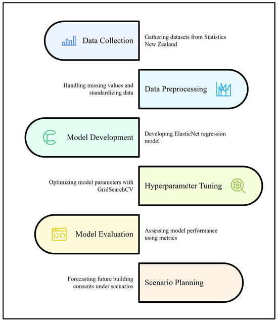
Figure 1.
Research methodology.
4. Results
4.1. Descriptive Statistics
The descriptive statistics (n = 23 years) highlight substantial variability across key economic and demographic indicators in New Zealand, as illustrated in Table 3. GDP averaged approximately NZD 215 billion, with a standard deviation of NZD 71.8 billion, while construction GDP averaged NZD 12.5 billion, indicating the sector’s significant but fluctuating contribution. Population metrics showed consistent growth, with the 40–64 age group averaging 1.4 million. Housing metrics, including standalone houses (mean: 18,568) and HPI (mean: 1776), exhibited notable dispersion, reflecting housing demand dynamics. Inflation-related indices (CGPI, PPI, and CPI) and the OCR also revealed significant temporal variations relevant for modelling macroeconomic impacts on construction trends.
Table 3.
Descriptive statistics of the variables adopted in this research.
4.2. Performance Measures
The performance of the ElasticNet regression models was assessed using the R-squared (R2), RMSE, and MAE. The results are summarised in Table 4. The retirement village model performed well, with an R2 of 0.878, indicating that 88% of the variance was explained, and a low RMSE (258.77) and MAE (225.93). The apartments model showed a moderate R2 of 0.681, with higher error metrics (RMSE: 843.89, MAE: 612.38), suggesting room for improvement. The multi-unit model had an excellent R2 of 0.910 but high error values (RMSE: 1483.70, MAE: 1050.68), indicating potential issues with prediction accuracy. The standalone houses model, with an R2 of 0.795, had the highest errors (RMSE: 1727.12, MAE: 1404.52), pointing to the need for significant refinement. In conclusion, the retirement village model performed best, while the others require further tuning to enhance accuracy and reduce errors.
Table 4.
Performance of the ElasticNet regression models.
4.3. Feature Importance
A feature importance analysis was conducted to identify the key predictors influencing building consent counts across four construction categories: retirement villages, apartments, multi-unit developments, and standalone houses. The importance of each feature was determined based on the magnitude of the coefficients from the ElasticNet regression model, with larger values indicating a more significant influence on the predicted outcomes. In the case of retirement villages, demographic features, particularly the 65 and over age group (importance: 237) and the 20–39 age group (importance: 229), were identified as the most influential factors, highlighting the importance of both the target demographic and potential caretakers or family members in the decision-making process. Additionally, the house price index (HPI) (importance: 205) emerged as a significant positive predictor, reflecting the influence of market conditions on the development of retirement communities, while the official cash rate (OCR) (importance: −157) exhibited a negative relationship, suggesting that higher borrowing costs may dampen investment in this sector. For apartments, the 20–39 age group (importance: 1443) remained a dominant positive predictor, confirming the high demand for apartments among younger, urban populations, while immigration (importance: 969) underscored the impact of population growth on housing demand, particularly in metropolitan areas. The HPI (importance: 305) showed a positive relationship, indicating that property market fluctuations strongly influence apartment developments. Conversely, unemployment (importance: −2301) demonstrated a substantial adverse effect, revealing the economic vulnerability of apartment projects to downturns. In the analysis of multi-units, the 20–39 age group (importance: 4725) once again emerged as the most significant predictor, driven by younger populations seeking multi-unit housing options. The HPI (importance: 4262) played a similarly important role, emphasising the crucial link between housing market dynamics and multi-unit development, while CPI home ownership (importance: 3,731) illustrated the impact of affordability on the demand for multi-unit housing. Unemployment (importance: −3168) negatively affected multi-unit developments, reinforcing the economic sensitivity of this category, while the 40–64 age group (importance: −6265) exhibited the largest negative influence, suggesting a preference mismatch between this demographic and multi-unit housing. For standalone houses, the 20–39 age group (importance: 4229) was the most influential positive predictor, consistent with the demand for single-family homes among younger families. The 65 and over age group (importance: 2708) also had a notable positive effect, reflecting the preference for larger, standalone homes among retirees. The HPI (importance: 3566) demonstrated a strong positive correlation with building consent, while unemployment (importance: −6668) showed the most substantial negative impact, emphasising the importance of economic stability for the approval of standalone housing projects.
Additionally, the PPI (inputs) (importance: 4336) indicated that rising construction costs negatively affect consent approvals. The analysis revealed several key insights. The 20–39 age group was a consistent positive predictor across all categories, illustrating its central role in driving housing demand; unemployment was a dominant negative predictor, underscoring the vulnerability of building consent approvals to economic fluctuations; and HPI was a significant positive predictor across all categories, highlighting the critical influence of real estate market conditions on housing development. Age-specific factors, particularly the 65 and over and 20–39 age groups, were key drivers for retirement villages and standalone houses, while economic factors such as the HPI and unemployment were universally influential. These findings contribute valuable insights for policymakers, urban planners, and construction stakeholders, providing a foundation for better predicting and managing consent processes in response to demographic, economic, and market conditions. Figure 2 illustrates the results of the socio-economic feature importance analysis conducted on the four residential types considered in this study.
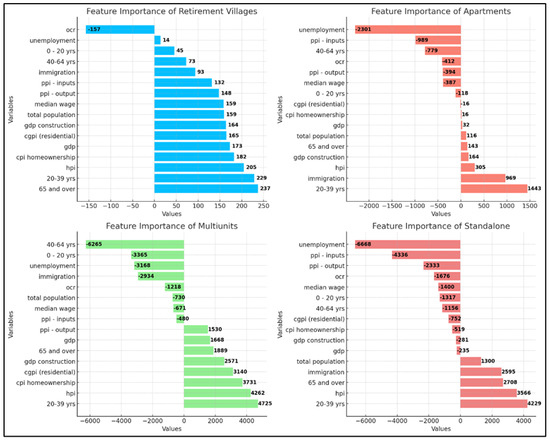
Figure 2.
Socio-economic feature importance for the residential construction types.
4.4. Residual Analysis
The residual analysis demonstrated that the residuals were approximately normally distributed, with a mean close to zero, indicating a well-calibrated model overall. However, signs of heteroscedasticity were observed, particularly in the categories of multi-unit development and standalone houses, where the residual variance increased with larger predicted values. This suggests that the model may not fully capture the increasing variability in these categories at higher prediction levels. Despite this, no discernible patterns of non-linearity or model misspecification were detected, and the residuals exhibited a random distribution, supporting the assumption of homoscedasticity for most building types. These findings imply that while the model demonstrates a generally strong fit, further refinement to address heteroscedasticity in specific categories may enhance predictive performance. The residual analysis results are shown in Figure 3.
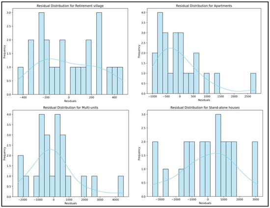
Figure 3.
Residual analysis distribution for the four residential types.
4.5. Five-Year Projections with Scenarios
The five-year projections for all building type consent counts are analysed under three distinct scenarios: optimistic, pessimistic, and realistic. Visually represented with colour differentiation, these projections provide a comprehensive outlook based on varying assumptions about the future economic and regulatory environment. Please note that the scenarios presented in this study are hypothetical, designed to showcase the practical implications of the developed model for projecting future housing demand. However, they can become more robust and realistic in the future as the scope expands. In the optimistic scenario (green), we anticipate robust consent growth driven by favourable economic conditions, increased urbanisation, and supportive housing policies. Conversely, the pessimistic scenario (red) forecasts a decline in consent, considering potential economic downturns, tightening regulations, and reduced demand for high-density living. The realistic scenario (blue) offers a balanced projection, assuming moderate growth aligned with current trends and ongoing market conditions. These projections underscore the significant influence of external factors on the apartment sector, with the optimistic and pessimistic scenarios providing clear bounds for potential growth. This comprehensive analysis highlights the need for flexibility in planning and decision-making, allowing stakeholders to prepare for a range of possible outcomes based on varying market dynamics and policy shifts. Figure 4 shows an example of the estimated projections, considering the scenario mentioned in Section 3.5.
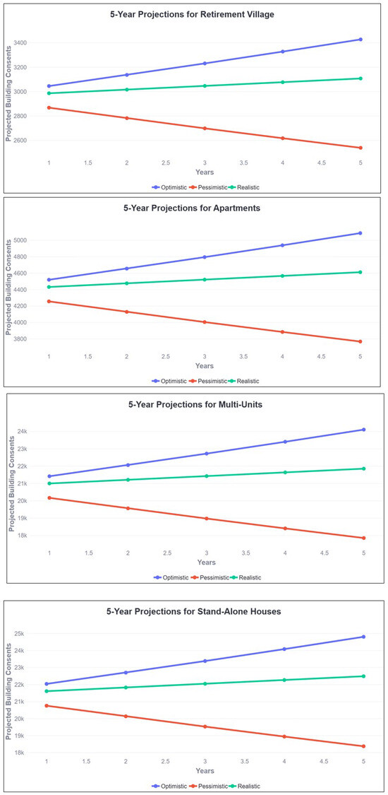
Figure 4.
Hypothetical scenario projections.
5. Discussion
5.1. General Discussion
Total population has long been adopted as a significant indicator in residential forecasting research [16,19,24]. The findings of this study suggest that disaggregating the total population into age brackets yields stronger indicators. This confirms the approach of Lindh and Malmberg [22], demonstrating that specific age groups, particularly the 20–39 and 65+ age groups, could have distinct influences on the demand for different residential types.
The 20−39 age group, encompassing the younger generations embarking on starting their professional and social lives, was a common significant predictor among the four types of residential buildings studied. The high predictive tendency of this indicator should guide urban planners, designers, and house providers to focus on housing solutions to satisfy the requirements of this age group, such as focusing on small- to medium-sized housing for new families and housing affordability. It also implies that as the 20–39 age group is mainly a working category and needs to be closer to business centres, high-density residential buildings such as apartment buildings and multi-unit housing may offer practical alternatives to satisfy the requirements of this age group. Rapid urbanisation and internal migration may exacerbate the effect of this working age group on residential demands and may be worthy of inclusion in future studies. Therefore, this age bracket, driven by employment accessibility, affordability, and lifestyle preferences, could highly influence the residential demand landscape.
Similarly, the 65+ age group was a substantial predictor for the retirement villages and standalone housing categories. With the ageing population characteristics in New Zealand, vigilant tracking and forecasting of this category is required to prepare suitable housing types, featuring accessibility options and proximity to essential services and utilities rather than business centres and work areas. The findings underscore the importance of using age groups as a predictor in forecasting future residential demand, enabling the provision of adequate and suitable housing categories to satisfy the demographic landscape of the population. It further highlights the deficiency of adopting specific age groups as indicators in residential planning and forecasting in previous research. Further breakdown into smaller age bracket categories may provide more accurate predictions of the residential preferences across age groups and highlight the points of changing preferences. However, this study did not consider the effects of changes in household composition, such as intergenerational living and extended family co-living, which may be common across some sectors of New Zealand’s population. Future studies may benefit from considering family structure variables to refine the demand projections.
Economic indicators also showed high predictive power. Interest rates (OCR) were observed to dampen demand across all the residential types, in harmony with other research [6,10,13,16,19]. Although other economic indicators, such as GDP and GDP for construction, exhibited a positive relationship with residential demand, as predicted by some studies [6,13,16,17,18,19,23], it was noticed that they were not among the most influential predictors in this study. This may affirm that housing demand will trend naturally and remain relatively inelastic to broader economic fluctuations, with demographic and market-specific variables exerting a stronger impact. Governmental and public housing bodies will continue to face significant funding challenges under such circumstances and must fulfil their responsibilities, even under scarce and constrained conditions.
Construction market conditions, which are closely related to the prevailing economic conditions, were also among the powerful indicators. The house price index (HPI) showed a strong positive relation with demand across all residential categories, similar to some findings [10,13,16,23]. While this metric indicates robust demand and benefits developers and project owners, it should be noted that it may signal affordability challenges, especially for the younger age brackets, as discussed. For policymakers, this suggests that affordability concerns should be considered in housing development policies so as not to disadvantage the younger generations and first-home buyers.
The role of construction costs, reflected in indicators such as the producer price index (PPI), highlights the sensitivity of housing demand to input cost fluctuations [12,16,23]. Although a negative relationship was expected throughout the four residential categories, PPI—inputs was positively correlated with retirement villages. PPI—output, reflecting a measure of profitability, was expected to have a positive relationship with residential construction demands. However, a discrepancy was also noticed in the categories of standalone houses and apartments, which showed a negative relationship. Rising construction costs due to escalated material prices and labour shortages may have outpaced market absorption. Supply chain disruptions, which often lead to cost inflation and project delays, exacerbate the situation, reducing the overall output. Economic factors, such as interest rates and inflation, have further dampened new housing investments, making construction less profitable despite demand. As a result, instead of boosting PPI output, these challenges have constrained growth in the standalone and apartment housing categories. Higher profitability often incentivises developers to over-invest in housing, potentially leading to oversupply in the standalone and apartment categories. This oversupply, a common concern in New Zealand’s real estate cycles, can reduce demand and price corrections, further discouraging new construction in these sectors. Urban density policies and changing consumer preferences also play a role; local councils in cities such as Auckland and Wellington have prioritised medium- and high-density housing to address shortages and improve affordability, reducing demand for standalone houses. Economic uncertainty and market conditions, including fluctuations in interest rates, add to the demand sensitivity for standalone and apartment housing. High interest rates and increased construction costs make these asset classes less attractive for developers and buyers alike, particularly in a country where the housing market relies heavily on mortgage financing. Collectively, these factors highlight the nuanced interplay of profitability, affordability, and market cycles in shaping housing demand in New Zealand, particularly for standalone houses and apartments.
On the social level, unemployment was seen to exhibit a negative relationship with residential demands in most cases, confirming the importance of including unemployment in residential forecasting studies, in harmony with previous findings [6,10,13,19]. It is expected that as unemployment rates increase, higher numbers of people will experience financial constraints. Moreover, rising unemployment rates often reflect the overall economic conditions of a nation, usually signalling a slowing economy and less affinity to investment and spending. Although residential demand increases were expected with increases in the median wage, a negative relationship could also be detected. This could be attributed to economic factors such as the inflation caused by the increased median wages, tax policy and taxation thresholds, and changes in spending behaviours and savings. This finding reaffirms that income levels could be an important influencing factor and warrants its inclusion in residential forecasting studies, as forwarded by Macpherson and Sirmans [9].
5.2. Study Limitations
This study has several limitations that need to be addressed in future research. Firstly, data availability is limited for machine learning model training, particularly specific to New Zealand’s residential construction sector. The selection of data variables was largely dependent on the availability of the datasets at the time of this study, which may not fully capture the wide range of factors affecting construction demand. It is recommended that future research use more comprehensive datasets. While our study was constrained to a 23-year timeframe due to data availability limitations, future research would benefit from more comprehensive datasets emerging in the current era of generative AI and machine learning technologies, which offer improved data completeness and accessibility. Additionally, the scenario planning in this paper relies on three predefined static assumptions, limiting its ability to reflect the inherent uncertainty in real-world conditions. A more robust approach could incorporate probabilistic techniques to model a wider range of possible outcomes and improve the performance of the projections. Furthermore, this study does not explicitly account for external shocks, such as economic downturns, policy changes, or supply chain disruptions, which could significantly impact real-world outcomes.
6. Conclusions
This study identified the main factors and variables that impact the demand for residential buildings in New Zealand. This study used data sourced from Statistics New Zealand regarding four main dimensions: demographic data, economic data, social factors data, and market conditions data. Each dimension included an array of different influencing factors. The model identifies demographic indicators, such as the 20−39 and 65+ age groups, and economic factors, such as the house price index and unemployment rates, as critical predictors across various building types. These findings emphasise integrating demographic trends and economic conditions into housing demand forecasting to enhance the sector’s resilience and adaptability. Policymakers and urban planners can leverage these insights to develop strategies addressing housing supply deficiencies, affordability challenges, and market dynamics, ultimately contributing to sustainable urban growth and accessibility.
The prominent and most influential factors were identified as demographic indicators, specifically the 20–39 and 65+ age groups, highlighting the importance of considering age groups rather than total populations. This study recommends further disaggregating age groups into smaller age brackets to refine the outputs. Economic factors such as the house price index and OCR were also identified as influential and critical factors in shaping the demand profiles of the four studied residential construction types, confirming the findings of previous studies.
Author Contributions
Conceptualization, J.O.B.R.; Methodology, T.P.; Validation, E.E. and T.P.; Formal analysis, E.E. and T.P.; Investigation, E.E. and T.P.; Resources, E.E.; Writing—original draft, E.E. and T.P.; Writing—review & editing, E.E. and J.O.B.R.; Visualization, T.P.; Supervision, J.O.B.R. All authors have read and agreed to the published version of the manuscript.
Funding
This research was funded by the Ministry of Business, Innovation, and Employment in New Zealand, grant number MAUX2005.
Data Availability Statement
The original contributions presented in the study are included in the article, further inquiries can be directed to the corresponding author.
Conflicts of Interest
The authors declare no conflict of interest.
References
- MBIE. Building and Construction Sector Trends-Annual Report 2023; Ministry of Business, Innovation, and Employment: Wellington, New Zealand, 2023. [Google Scholar]
- MBIE. National Construction Pipeline Report 2023: A forecast of Building and Construction Activity; Ministry of Business, Innovation, and Employment: Wellington, New Zealand, 2023. [Google Scholar]
- Huang, T.; Katz, A.; Dunn, T. Housing Availability and Affordability: A Case Study on the Canterbury Region; New Zealand Institute of Economic Research: Wellington, New Zealand, 2024. [Google Scholar]
- Johnson, A.; Howden-Chapman, P.; Eaqub, S. A Stocktake of New Zealand’s Housing. 2018. Available online: https://www.beehive.govt.nz/sites/default/files/2018-02/A%20Stocktake%20Of%20New%20Zealand%27s%20Housing.pdf (accessed on 11 January 2025).
- MHUD. The Housing Dashboard: Public Housing Register. Available online: https://www.hud.govt.nz/stats-and-insights/the-government-housing-dashboard/housing-register (accessed on 11 January 2025).
- Ng, S.T.; Skitmore, M.; Wong, K.F. Using genetic algorithms and linear regression analysis for private housing demand forecast. Build. Environ. 2008, 43, 1171–1184. [Google Scholar]
- Lam, K.C.; Oshodi, O.S. Using univariate models for construction output forecasting: Comparing artificial intelligence and econometric techniques. J. Manag. Eng. 2016, 32, 04016021. [Google Scholar] [CrossRef]
- Van Wee, B. Large infrastructure projects: A review of the quality of demand forecasts and cost estimations. Environ. Plan. B Plan. Des. 2007, 34, 611–625. [Google Scholar] [CrossRef]
- Macpherson, D.; Sirmans, S. Forecasting seniors housing demand in Florida. J. Real Estate Portf. Manag. 1999, 5, 259–274. [Google Scholar] [CrossRef]
- Fan, R.Y.; Ng, S.T.; Wong, J.M. Reliability of the Box–Jenkins model for forecasting construction demand covering times of economic austerity. Constr. Manag. Econ. 2010, 28, 241–254. [Google Scholar] [CrossRef]
- Tang, J.C.; Karasudhi, P.; Tachopiyagoon, P. Thai construction industry: Demand and projection. Constr. Manag. Econ. 1990, 8, 249–257. [Google Scholar] [CrossRef]
- Goh, B.H. Residential construction demand forecasting using economic indicators: A comparative study of artificial neural networks and multiple regression. Constr. Manag. Econ. 1996, 14, 25–34. [Google Scholar]
- Akintoye, A.; Skitmore, M. Models of UK private sector quarterly construction demand. Constr. Manag. Econ. 1994, 12, 3–13. [Google Scholar] [CrossRef]
- Grimes, A.; Hyland, S. Housing markets and the global financial crisis: The complex dynamics of a credit shock. Contemp. Econ. Policy 2015, 33, 315–333. [Google Scholar] [CrossRef]
- Jiang, H.; Jin, X.-H.; Liu, C. The effects of the late 2000s global financial crisis on Australia’s construction demand. Australas. J. Constr. Econ. Build. 2013, 13, 65–79. [Google Scholar] [CrossRef]
- Sammour, F.; Alkailani, H.; Sweis, G.J.; Sweis, R.J.; Maaitah, W.; Alashkar, A. Forecasting demand in the residential construction industry using machine learning algorithms in Jordan. Constr. Innov. 2024, 24, 1228–1254. [Google Scholar] [CrossRef]
- Green, R.K. Follow the leader: How changes in residential and non-residential investment predict changes in GDP. Real Estate Econ. 1997, 25, 253–270. [Google Scholar] [CrossRef]
- Chase, C.W. Demand-Driven Forecasting: A Structured Approach to Forecasting; John Wiley & Sons: Hoboken, NJ, USA, 2013. [Google Scholar]
- Jiang, H.; Liu, C. A panel vector error correction approach to forecasting demand in regional construction markets. Constr. Manag. Econ. 2014, 32, 1205–1221. [Google Scholar] [CrossRef]
- Kim, K.-B.; Cho, J.-H.; Kim, S.-B. Model-based dynamic forecasting for residential construction market demand: A systemic approach. Appl. Sci. 2021, 11, 3681. [Google Scholar] [CrossRef]
- Engerstam, S.; Warsame, A.; Wilhelmsson, M. Exploring the effects of municipal land and building policies on apartment size in new residential construction in Sweden. J. Risk Financ. Manag. 2023, 16, 220. [Google Scholar] [CrossRef]
- Lindh, T.; Malmberg, B. Demography and housing demand—What can we learn from residential construction data? J. Popul. Econ. 2008, 21, 521–539. [Google Scholar] [CrossRef]
- Goh, B.H. The dynamic effects of the Asian financial crisis on construction demand and tender price levels in Singapore. Build. Environ. 2005, 40, 267–276. [Google Scholar] [CrossRef]
- Goh, B.H.; Pin, T.H. Forecasting construction industry demand, price and productivity in Singapore: The BoxJenkins approach. Constr. Manag. Econ. 2000, 18, 607–618. [Google Scholar]
- Nikodinoska, D.; Käso, M.; Müsgens, F. Solar and wind power generation forecasts using elastic net in time-varying forecast combinations. Appl. Energy 2022, 306, 117983. [Google Scholar] [CrossRef]
- Shah, I.; Iftikhar, H.; Ali, S. Modeling and forecasting electricity demand and prices: A comparison of alternative approaches. J. Math. 2022, 2022, 3581037. [Google Scholar] [CrossRef]
- Tian, F.; Yang, Y.; Mao, Z.; Tang, W. Forecasting daily attraction demand using big data from search engines and social media. Int. J. Contemp. Hosp. Manag. 2021, 33, 1950–1976. [Google Scholar] [CrossRef]
- Liu, W.; Dou, Z.; Wang, W.; Liu, Y.; Zou, H.; Zhang, B.; Hou, S. Short-term load forecasting based on elastic net improved GMDH and difference degree weighting optimization. Appl. Sci. 2018, 8, 1603. [Google Scholar] [CrossRef]
- Goh, B.H. Forecasting residential construction demand in Singapore: A comparative study of the accuracy of time series, regression and artificial neural network techniques. Eng. Constr. Archit. Manag. 1998, 5, 261–275. [Google Scholar] [CrossRef]
- Skribans, V. Construction Industry Forecasting Model. 2002. Available online: https://mpra.ub.uni-muenchen.de/16365/ (accessed on 13 March 2025).
- Kissi, E.; Adjei-Kumi, T.; Badu, E.; Boateng, E.B. Factors affecting tender price in the Ghanaian construction industry. J. Financ. Manag. Prop. Constr. 2017, 22, 252–268. [Google Scholar] [CrossRef]
- Kissi, E.; Adjei-Kumi, T.; Amoah, P.; Gyimah, J. Forecasting construction tender price index in Ghana using autoregressive integrated moving average with exogenous variables model. Constr. Econ. Build. 2018, 18, 70–82. [Google Scholar] [CrossRef]
- Oteng, P.A.; Lartey, V.C.; Amofa, A.K. Modeling the Macroeconomic and Demographic Determinants of Life Insurance Demand in Ghana Using the Elastic Net Algorithm. SAGE Open 2023, 13, 21582440231196658. [Google Scholar] [CrossRef]
- Sloboda, B.; Pearson, D.; Etherton, M. An application of the LASSO and elastic net regression to assess poverty and economic freedom on ECOWAS countries. Math. Biosci. Eng. 2023, 20, 12154–12168. [Google Scholar] [CrossRef]
- Wang, Q.; Hall, G.J.; Zhang, Q.; Comella, S. Predicting implementation of response to intervention in math using elastic net logistic regression. Front. Psychol. 2024, 15, 1410396. [Google Scholar] [CrossRef]
- Ebrahimi, V.; Bagheri, Z.; Shayan, Z.; Jafari, P. A machine learning approach to assess differential item functioning in psychometric questionnaires using the elastic net regularized ordinal logistic regression in small sample size groups. BioMed Res. Int. 2021, 2021, 6854477. [Google Scholar] [CrossRef]
- Muoki, M.M. A Systematic comparison of performance of Ridge, Lasso, Elastic net and Relaxed Elastic net when fitting high dimensional data for sales prediction. Ph.D. Thesis, Strathmore University, Nairobi, Kenya, 2022. [Google Scholar]
- Zhao, S.; Lai, Y.; Ye, C.; Lee, K. Machine learning applications in household-level demand prediction. Appl. Econ. Lett. 2024, 31, 5–11. [Google Scholar] [CrossRef]
Disclaimer/Publisher’s Note: The statements, opinions and data contained in all publications are solely those of the individual author(s) and contributor(s) and not of MDPI and/or the editor(s). MDPI and/or the editor(s) disclaim responsibility for any injury to people or property resulting from any ideas, methods, instructions or products referred to in the content. |
© 2025 by the authors. Licensee MDPI, Basel, Switzerland. This article is an open access article distributed under the terms and conditions of the Creative Commons Attribution (CC BY) license (https://creativecommons.org/licenses/by/4.0/).