Article

Bearing Capacity Prediction of Cold-Formed Steel Columns with Gene Expression Programming

1
China Railway Construction Group Co., Ltd., East China Engineering Co., Ltd., Suzhou 215300, China
2
Faculty of Architecture and Civil Engineering, Huaiyin Institute of Technology, Huaian 223001, China
*
Author to whom correspondence should be addressed.
Buildings 2025, 15(10), 1597; https://doi.org/10.3390/buildings15101597
Submission received: 10 April 2025 / Revised: 30 April 2025 / Accepted: 7 May 2025 / Published: 9 May 2025
(This article belongs to the Special Issue Application of Experiment and Simulation Techniques in Engineering)

Abstract

In recent years, there has been a growing use of cold-formed steel (CFS) structures in the field of civil engineering. The objective of this study is to utilize gene expression programming (GEP) in order to forecast the ultimate bearing capacity of cold-formed steel columns. The buckling resistance of built-up back-to-back cold-formed (BCF) thin-walled tube columns under axial compression, and of cold-formed thick-walled steel columns under combined axial compression and bending, is examined in this paper. The data were collected from various studies to develop and verify the proposed model, with training and testing sets of 160 and 14, and 2000 and 500, respectively. The performance of the genetically developed GEP models was evaluated and compared with that of the mechanical models specified in American and Chinese specifications. The GEP models demonstrated significantly better performance compared with that of the code-specified models. The results generated by the GEP models demonstrate stronger alignment with both experimental data and analytical predictions. This study also demonstrates the capability of the GEP models to calculate the ultimate bearing capacity, with the proposed mechanical models being used as a reference for calculations.

1. Introduction

Cold-formed steel structures, known for their corrosion resistance, high strength-to-weight ratio, and ease of fabrication and assembly, have been increasingly employed in civil engineering applications. Typically, cold-formed thin-walled components are composed of single channels, which, by virtue of their low torsional and flexural rigidities, have restricted load-bearing capacities. Engineers frequently employ BCF members for applications requiring greater load-bearing capacities. Despite their importance in the practical design of BCF members, the CFS design specifications outlined in [1,2] exhibit several limitations. Firstly, Stone et al. [3] found that the use of the modified slenderness ratio for predicting the compressive capacity of BCF members is excessively conservative and leads to significant discrepancies of 16–65% between test results and design specifications. According to the findings of Roy et al. [4], it has been demonstrated that the existing design criteria are insufficiently conservative, as they underestimate the required strength of short BCF compression members by approximately 12%. This discrepancy mostly arises from the failure mode of local buckling. In addition, prior studies [5,6] have provided evidence that the material properties of cold-formed steel sections with a thickness above 6 mm exhibit notable distinctions compared to thin-walled sections. In a study by Tong et al. [7] on cold-formed thick-walled square hollow sections with a thickness greater than 6 mm, it was demonstrated that longitudinal residual stresses exhibit a nonlinear distribution through the wall’s thickness. The existing design requirements have yet to incorporate the distinct material characteristics of cold-formed steel sections for determining member strength in the design process. In addition, there is a notable absence of detailed testing and verification data for these components, which presents difficulties in precisely assessing their structural capabilities and behaviors. The lack of comprehensive experimental data pertaining to the strength, deformation properties, and failure mechanisms of the subject under consideration presents a challenge for designers who want to depend only on existing design guidelines.
In light of these challenges, many scholars often turn to traditional experimental approaches and finite element simulations to formulate new recommendations and refine existing specifications. However, traditional experimental tests are affected by high costs, long test cycles, and limited reproducibility. On the other hand, finite element simulations often require significant computational resources and time. Gene expression programming (GEP), an optimization method rooted in genetics and natural selection principles, was subsequently introduced. Compared with other machine learning methods, the primary advantage of GEP over regression tools lies in its ability to generate equations without making assumptions on prior information of existing relationships [8], making GEP interpretable. The equations are formed by extracting more meaningful information from all of the underlying parameters, avoiding the influence of other, irrelevant parameters. GEP is found to be easier to implement, quicker to create, and requires minimal processing during iteration. Such equations, which are robust and not confined to the range of existing parameters, have been illustrated by several researchers. For instance, Mario et al. [9] demonstrated that the GEP method has great potential for predicting the rotational capacity of cold-formed rectangular and square hollow section beams, Abdulkadir [10] utilized genetic programming to derive a novel formula for the breaking strength of cold-formed steel webs, and Mohammad et al. [11] evaluated the damage to H-section steel columns under impulsive blast loads via GEP. In addition, GEP can be extended by adding new genes or adjusting the parameters, thus making it possible to apply it to a broader range of fields.
In this study, GEP was used to predict the ultimate bearing capacity and generate formulae for the buckling resistance of BCF thin-walled tube columns under axial compression and cold-formed thick-walled steel columns under combined axial compression and bending. Finally, the results derived from GEP were compared with the existing design specifications, experimental results, and finite element simulation results. The comparison demonstrated that the formulae proposed by GEP aligned more closely with the experimental and finite element analysis data. Compared to the mechanical models specified in existing design specifications, the GEP prediction models are not required to consider additional factors and are shown to possess superior accuracy and performance.

2. Model Parameters

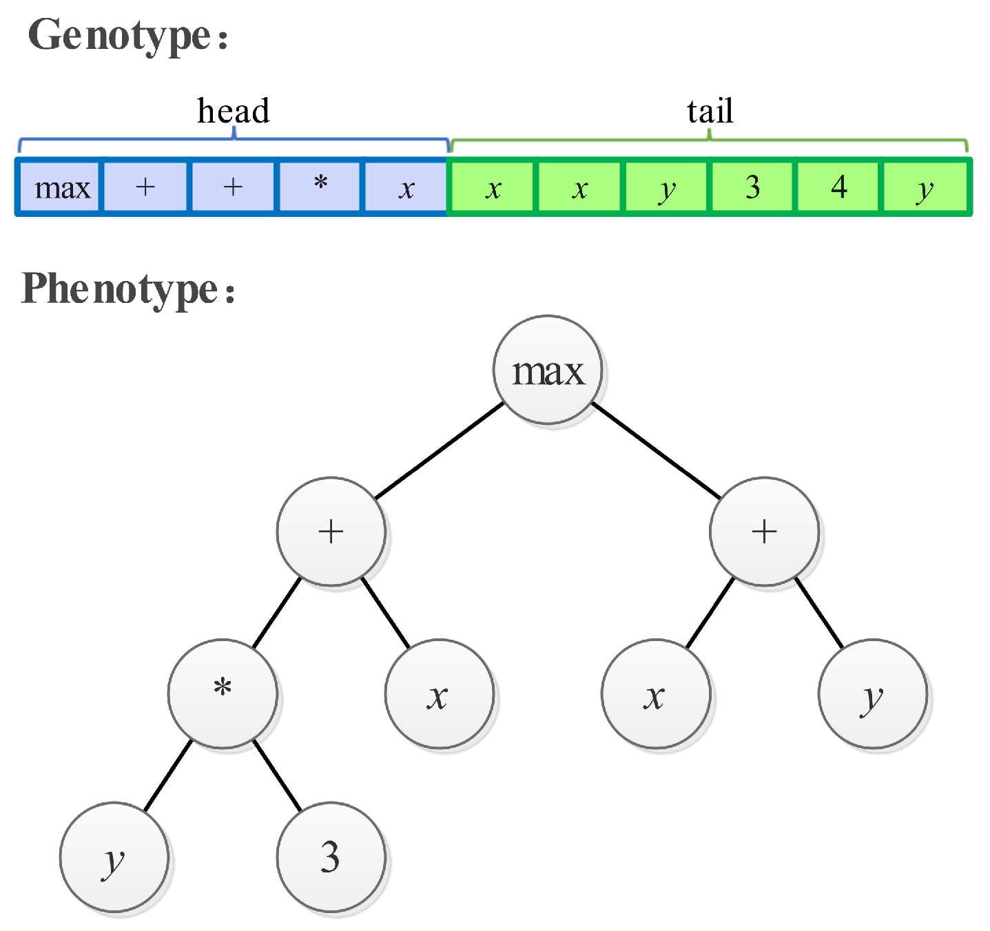
2.1. Gene Expression Programming

The initial development of GEP can be attributed to Cândida Ferreira [12] in 2001. The algorithm is an innovative and adaptive approach that draws inspiration from the structural and functional aspects of biological genes. It is a synthesis of genetic algorithms (GAs) and genetic programming (GP), effectively combining the strengths of both methods while also addressing their limitations. In recent years, the research community has shown growing interest in the field of GEP, resulting in the emergence of many methodologies designed to improve its functionalities.
GEP has two expression modes, namely, genotype and phenotype. The two expressions, max = (3y + x, x + y), are shown in Figure 1. From the evolutionary point of view, connecting sub-expression trees with a specific linkage function is simple and efficient. This approach can significantly improve the efficiency of systems from single-gene systems to multi-gene systems, providing solutions to different problems. It should be noted that the “*” in the figure represents “×”.

2.2. Fitness Function

To relieve deception in genetic algorithms, the methods of tabu search [13], simulated annealing [14], and space partitioning [15] have been used to maintain the diversity of GEP populations and improve the local search ability and accuracy of GEP. In addition, since GEP determines whether individuals are inherited into the next generation group through fitness, the transformation of the fitness function can also optimize GEP. To minimize the error in prediction, the average relative error is used to evaluate the performance of the models, as shown in Equation (1). Originating from the idea of simulated annealing, the function is exponentially transformed to reduce the fitness of early above-normal individuals, which enables GEP to jump out of the local optimum phenomenon as early as possible, and the final fitness function is shown in Equation (2).
X = i = 1 n ( a i p i / p i ) / n
F x = exp ( x ) × 1000
where p is the predicted result, and a is the actual result.

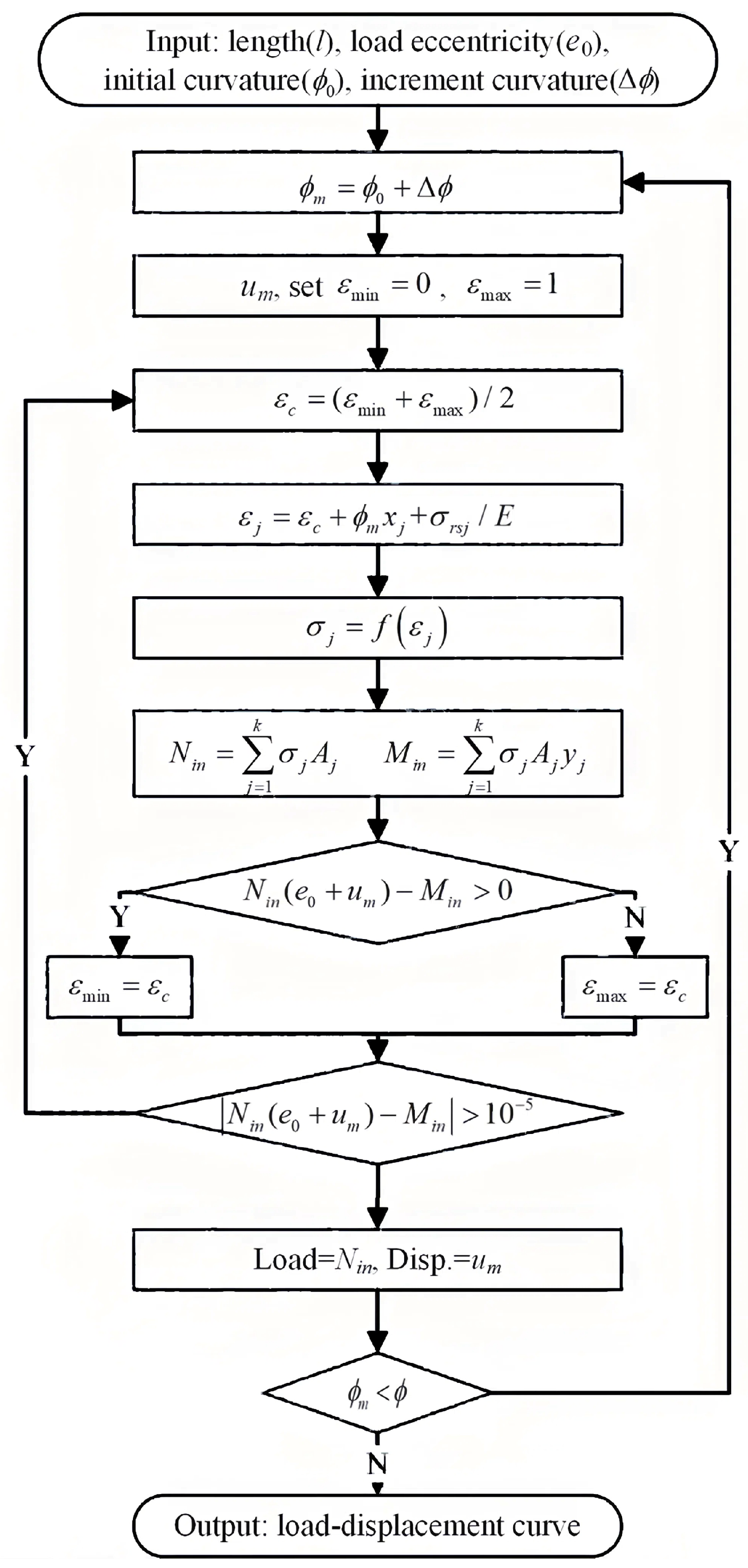
2.3. Modeling Process

GEP randomly creates the initial population chromosomes and then calculates the fitness of individuals one by one to assess whether the requirements of the final evolutionary goal are met. If the fitness meets the target, the best individual is output as the optimal model. Otherwise, individuals are selected using a round-robin sampling strategy (i.e., the fittest individual is selected and inherited to the next generation with a higher probability) and evolved using genetic operators (e.g., replication, mutation, transposition, and recombination) to generate a new population. Evolution is repeatedly evaluated until the conditions for termination are met, as shown in Figure 2. The general parameters of GEP are set as shown in Table 1.
To assess the prediction performance of the model, R-squared (R2), Root-Mean-Square Error (RMSE), and Relative Absolute Error (RAE) are chosen as the evaluation indicators, as shown in Equations (3)–(5). As R2 approaches 1, the values of RMSE and RAE decrease, indicating better prediction results of the model.
R 2 = 1 i = 1 n p i a i 2 / i = 1 n a i a ¯ 2
R M S E = ( i = 1 n ( p i a i ) 2 ) / n
R A E = i = 1 n p i a i / i = 1 n a i a ¯
where p is the predicted result, a is the actual result, and ā is the average.

3. Buckling Resistance of BCF Thin-Walled Tube Columns Under Axial Compression

3.1. Finite Element Analysis

3.1.1. General

To predict the behaviors and compressive capacities of BCF tube columns, and to develop finite element (FE) models of the tested specimens, version 2021 of the Abaqus/CAE software [16] was utilized. In the FE model, S4R shell elements were used. Two stages comprised the FE analyses. The columns were initially subjected to eigenvalue deformation analyses. By integrating the initial geometric imperfections into nonlinear analyses, the ultimate loads and deformed morphologies were determined in accordance with the first eigenvalue buckling modes. Finally, the static/general solver was implemented with a specific damping factor of 0.0005 and a maximum stabilization ratio of 0.005, due to the complexity of the section geometry and contacts in each column. Using the validated FE models, additional numerical data were generated through parametric studies, which were subsequently conducted utilizing the experimental results that had been utilized to assess the accuracy and dependability of the FE model.

3.1.2. Material Properties

The corresponding true stress-versus-strain curve was used in the FE models. This conversion is described by Equations (6) and (7), where σtrue represents the true stress, σeng represents the engineering stress, εpl represents the true plastic strain, εeng represents the engineering strain, and E represents the elastic modulus:
σ t r u e = σ e n g ( 1 + ε e n g )
ε p l = ln ( 1 + ε e n g ) σ t r u e / E
The material properties were set to a yield strength and ultimate strength of 615 MPa and 625 MPa, respectively, with an elastic modulus of 20,500 MPa and a Poisson’s ratio of 0.3. The data were obtained through experiments on 0.95 mm thick G550 steel, using the method of Rokilan and Mahendran [17]. In accordance with Schafer and Peköz’s [18] recommendations, residual stresses were excluded from this study.

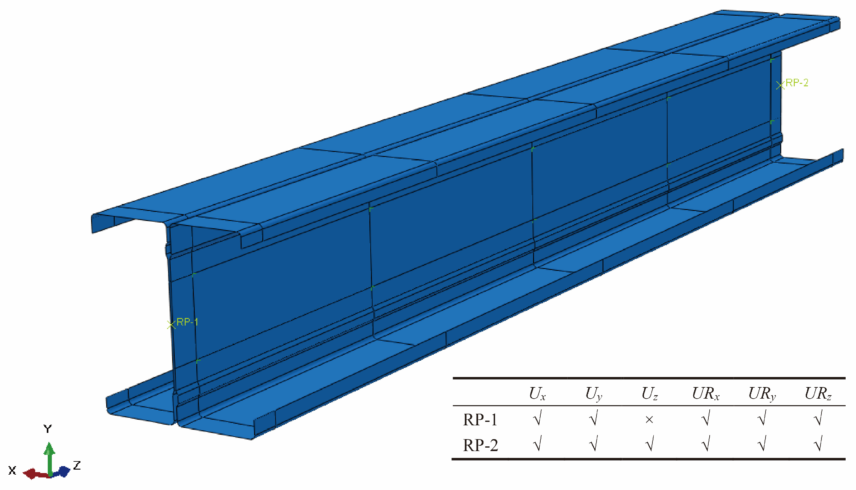
3.1.3. Boundary Conditions and Loading Method

All of the finite element models of the columns in this work utilized fixed-end support boundary conditions, as depicted in Figure 3. The symbol “√” denotes constraint, whereas “×” indicates freedom. The reference point (RP-1 or RP-2) is the centroid of the section, and the constraint on the end section is achieved through coupling. The application of axial compression loading through RP-1 involves the utilization of displacement control.

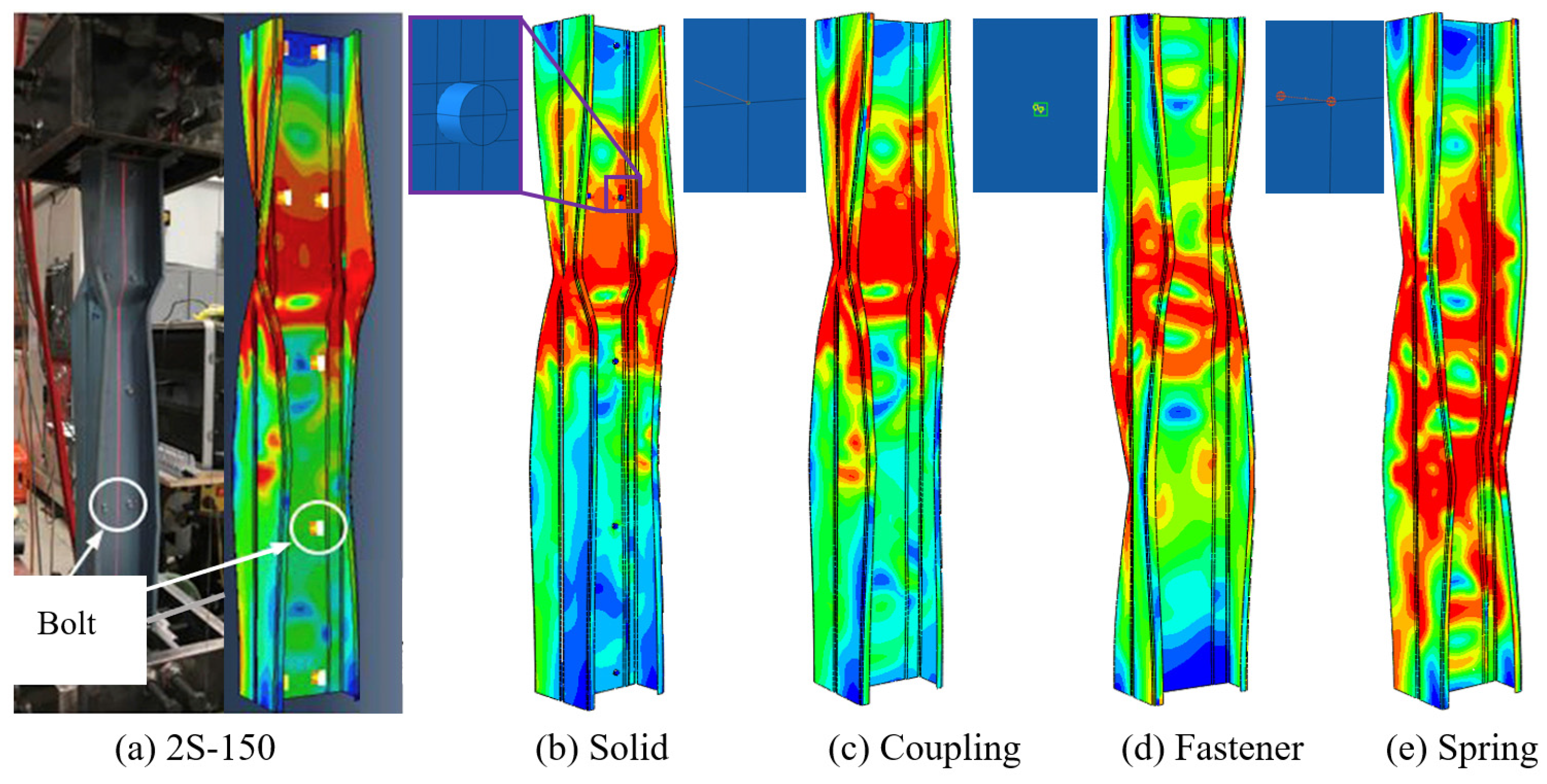
3.1.4. Contact and Bolt Simplification

The intricate configuration of the built-up back-to-back section introduced complexity into the interrelationships among elements within each member. Consequently, the “general contact” and “hard contact” normal behaviors were utilized. It was assumed that the coefficient of friction between individual components was 0.19 [19].
Modeling can be simplified by focusing on the compressive strengths and failure modes of the columns, rather than the failure modes of the bolts. To the best of the authors’ knowledge, there are four ways to model bolts. These models include solid modeling, coupling [20], “point-based” fasteners [21], and discrete spring models [22]. The results of comparing these four bolt simulation methods are shown in Figure 4 and Table 2.
The results show that the method using solid modeling has the highest error, while the other three methods have similar errors, all around 3%. However, the deformation mode simulated using the fastener and spring methods is somewhat inconsistent with the experiment results, so the coupling method was chosen to simulate the bolts.

3.1.5. Initial Geometric Imperfections and Residual Stresses

The determination of the comparable starting geometric imperfection was based on reference [23] for local buckling, which is b/100. The omission of residual stresses in finite element (FE) models can be attributed to findings from previous research investigations [24,25], which indicate that the impact of residual stresses on the ultimate loads of CFS members is negligible.

3.1.6. Mesh Sensitivity Analysis

In addition, a mesh sensitivity investigation was completed, as shown in Figure 5. To guarantee that the inaccuracy was within 3.5% in this investigation, the mesh size throughout the plate width was at least 5 mm.

3.1.7. Verification of FE Model

To validate the developed FE model, a comparison was made between its numerical and experimental results [21,25]. Furthermore, the load–deflection curves and failure modes derived from the finite element (FE) analysis were juxtaposed with the experimental findings, as shown in Figure 4, Figure 5 and Figure 6. The final loads predicted by the FE analyses and those determined by the experiments corresponded exceptionally well. In contrast, the FE analyses yielded steeper gradients for the load-versus-shortening curves compared to the test results. This discrepancy can be attributed to two factors: (1) distinct bolt simulation methodologies, and (2) localized flaws and variations along the length of the specimen. In summary, the developed finite element (FE) model demonstrates the ability to generate precise and dependable prognostications regarding the bowing capacity of BCF thin-walled columns.

3.1.8. Parametric Studies

The verified finite element model was utilized to perform a number of parametric investigations in the subsequent sections. The columns were assembled using C-shaped steel with rolled edges, according to the specifications. According to Son Tung Vy et al. [21], neither the bolt size nor the number of bolts per row substantially affects the load capacity. Therefore, the bolts were arranged in two rows along the height of the web, at one-quarter and three-quarters of the web height, respectively. The bolts were arranged in equal spacing, with three along the length of the member, as shown in Figure 7. To ensure local buckling of the tube column, the length of the column was taken as 1.2 times the height of the web. Various height–thickness and width–thickness ratios were selected to cover columns with various cross-sections, as shown in Table 3. All of the components were analyzed using CUFSM to ensure that the buckling mode was local buckling. Finally, a total of 800 sets of finite element numbers were established.

3.2. GEP Model Development

To save computer resources and optimize the model structure, input parameters were optimally selected using the random forest algorithm. The selection criteria were based on higher feature importance. The results of the parameter analysis are shown in Figure 8. The parameters of all columns are summarized in Table 4. A total of 160 sets of finite element data were used in the training set, and 14 sets of experimental data [25,26,27] were used in the test set to ensure the reliability and accuracy of GEP.
The function set F = {+, −, ×/, Q, ^2} was used, where Q represents the square root function. The number of genes was two, the head length was 12, the linking function was multiplication, and the remaining settings were the same as in Table 1. Figure 9 demonstrates the ETs resulting from the model. Sub-ET1 corresponds to Equation (8), and Sub-ET2 corresponds to Equation (9). The formulae of back-to-back built-up cold-formed steel columns based on GEP are shown in Equation (10).
F u , G E P , 2 1 = A t L + 2.58 h A 2 L / L 2
F u , G E P , 2 2 = f y t + 9.73 L / 1.96 b b 2 / t h
F u , G E P , 2 = F u , G E P , 2 1 × F u , G E P , 2 2
The existing specifications for cold-formed thin-walled steel mainly include the effective width method (EWM) and the direct strength method (DSM). The EWM calculates the effective width of structural components, which discounts their area. In contrast, the DSM entails adjusting the yield strength of the member. After checking Equations (8)–(10) proposed by GEP, we observed that these equations account for both the member area and yield strength adjustment. Specifically, Equation (8) incorporates the thickness, length, and height of the member to adjust its area, due to their influence on the flexural behavior of members. Similarly, Equation (9) adjusts the yield strength of the member by considering its thickness, width-to-thickness ratio, and height-to-width ratio.

3.3. Performance Analysis and Model Validity

  • Effective Width Method
By consulting the design provisions for axially compressed members in American code chapter C4 of AISI S100 2016 [1], one can determine the maximum concentric axial compression strength of columns using the EWM, through Equations (11) and (12):
P n = A e × F n = A e i × F n = b e i t × F n
b e = ω ,   λ 0.673 1 0.22 / λ ω / λ ,   λ > 0.673
where Fn is the compressive stress, λ is the flexibility coefficient of the plate, ω is the width of the plate, and be is the effective width of the plate.
The maximum concentric axial compression strength, as specified by the EWM in GB 50018-2002 [28], can be calculated using Equations (13) and (14):
P n = φ A e f y = φ × A e i × f y = φ × b e i t × f y
b e = b c ,   b 18 α ρ t 21.8 α ρ b / t 0.1 b c ,   18 α ρ t < b < 38 α ρ t 25 α ρ b / t b c ,   b > 38 α ρ t
where φ is the stability factor of the column under concentric axial compression, b is the width of the plate, be is the effective width of the plate, bc is the width of the compressive zone, and α and ρ are calculational coefficients.
2.
Direct Strength Method
In the American specification AISI S100 2016, the direct strength method is proposed to account for the interactions between flexural buckling, local buckling, and distortional buckling, as given in Equations (15)–(20) where Pne, Pnl, and Pnd are the nominal axial strengths for the flexural buckling, local buckling, and distortional buckling of the column under axial compression, respectively:
P n = min φ c P n e ,   φ c P n l ,   φ c P n d
P n e = 0.658 λ c 2 × f y ,   λ e 1.5 0.877 / λ c 2 × f y ,   λ e > 1.5
P n l = P n e ,   λ l 0.776 1 0.15 P c r l / P n e 0.4 P c r l / P n e 0.4 P n e ,   λ l > 0.776
P n d = P y ,   λ d 0.516 1 0.25 P c r d / P y 0.6 P c r d / P y 0.6 P y ,   λ d > 0.516
P c r , i = A g × f c r , i i = e ,   l ,   d
λ i = P n e / P c r , i ,   i = l   P y / P c r , i ,   i = e , d
where φc is the resistance coefficient of the axial compression member (generally 0.85), and fcr,i is the critical elastic buckling stress, which can be calculated via the finite-strip program CUFSM.
The results were calculated using methods from both AISC S100 2016 and GB 50018-2002, as shown in Figure 10, which contains data from both the training and test sets. FEA is the finite element simulation result in the training set, while Fu is the experimental result in the test set. The vertical coordinates represent calculation results from various specifications, GEP predictions, and finite element simulations or experimental results. The horizontal coordinate indicates the data number for each column. The statistical parameters of various models are listed in Table 5.
Figure 10 shows that the ultimate bearing capacities calculated by the EWM for the two specifications are very close and conservative. In Table 5, the results show that the average value of the ratio between the ultimate bearing capacities calculated by the EWM and finite element analysis results is only approximately 0.7. The calculation results of the DSM are also conservative, but they align with the numerical distribution studied. The error may be due to the fact that only a single member is used when using CUFSM software (v5.05) to calculate fcr,i, and the splicing effect of bolts is not considered, leading to lower fcr,i results. The phenomenon of being too conservative in the training set may be because the effective length is only 1.2 times the web height to suppress the distortional buckling, which does not exclude the constraint of local buckling. However, even in this case, GEP has an excellent prediction effect and can almost accurately estimate the ultimate bearing capacity.
For the test set, the experimental data of some scholars [25,26,27] were used for comparison. Table 6 lists the details of the experimental specimens and compares the ultimate bearing capacity between the experiments and GEP. The lengths of the tube columns in the test set were all three times the web height recommended by the Structural Stability Research Council to avoid constraining local buckling. However, from the experimental observations, despite the components exhibiting varying degrees of local-distortion-related buckling, the GEP-calculated mean reached 0.977, and R2 reached 0.951, providing a more accurate estimation of the ultimate bearing capacity. It is worth noting that a possible reason for the large errors in some data is that some parameters of the experimental components exceeded the range of the training set. Finally, GEP performed better than the existing design specification on both the training and test sets.

4. Buckling Resistance of Cold-Formed Thick-Walled Steel Columns Under Combined Axial Compression and Bending

4.1. Database

To the best of the authors’ knowledge, there remains a scarcity of experimental data pertaining to cold-formed thick-walled steel beam-columns. However, Zhou et al. [29] proposed a fiber model to estimate the buckling resistance of cold-formed thick-walled steel columns, and they verified its accuracy experimentally. Compared with using finite element software modeling to build datasets, the fiber model can greatly reduce the calculation time and converge more efficiently while ensuring accuracy.
The flowchart of the fiber model is shown in Figure 11. The fiber model first generates curvature using the input parameters and then calculates lateral displacement (um) at the mid-height. Based on constitutive models and the corresponding strains in the cross-section from εc and φm, the internal axial force (Nin) and bending moment (Min) are derived. Finally, using the binary search technique and force equilibrium, the load and lateral displacement are determined for a given curvature.
A comparison of experimental data from some scholars with the fiber model data is shown in Table 7. The fiber model can be considered to be correct within the error range. A total of 2500 direct-formed cold-formed thick-walled square steel columns were built using the fiber model. To consider the influence of residual stress and the cold bending effect, the constitutive model proposed by Hou [5] was used. The types of steel considered were Q235 and Q345. The cross-sectional dimensions of the components were all taken from research by other scholars [30,31,32,33]. The non-dimensional slenderness was set to 0 to 2.5, and the global geometric imperfection was L/1000, where L is the member length. The stress–strain relationship was the Ramberg–Osgood relation. The parameters of all columns are summarized in Table 8.

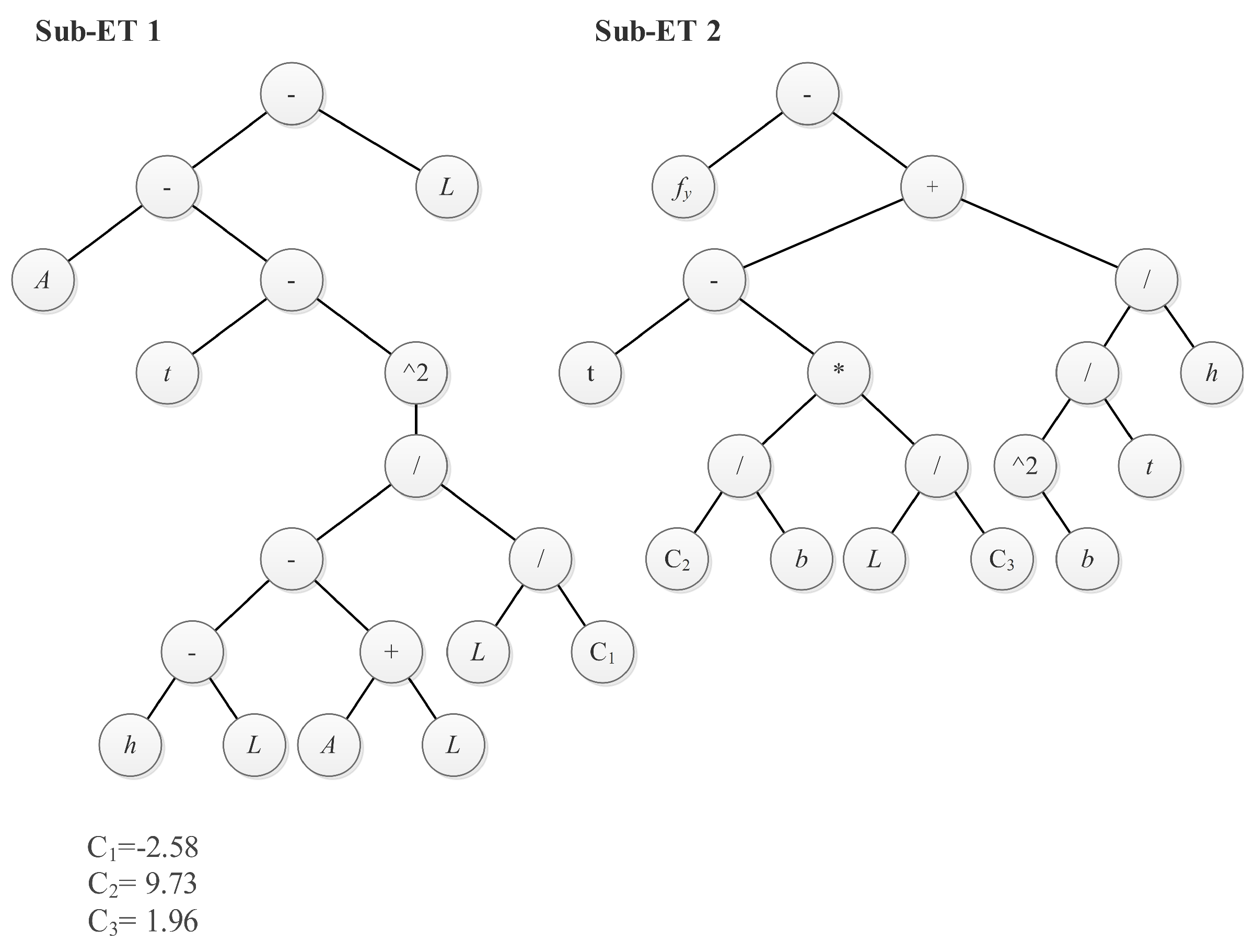
4.2. GEP Model Development

Similarly, the random forest algorithm was used to select the input parameters. The results of the parameter analysis are shown in Figure 12. The training and testing sets were 2000 and 500, respectively.
To make the formula derived from GEP closer to the specification and more interpretable, two custom functions (F1 and F2) were applied, as shown in Equations (21) and (22), respectively. Therefore, the set of functions was F = {F1, F2, +, ×, exp, ×4}, where *4 represents x1 × x2 × x3 × x4, and xn is the input parameter. After 20,000 generations of genetic evolution, the optimal combination of parameters included a gene number of two, a head length of eight, and the division linking function. The expression tree (ET) generated by this model is shown in Figure 13. Expression tree 1 (Sub-ET1) corresponds to Equation (23), and Sub-ET2 corresponds to Equation (24). The cold-formed thick-walled buckling resistance equation under combined axial compression and bending, proposed based on GEP, is shown in Equation (25).
F 1 = C 1 + C 2 x 1 x 2 2 / ( π 2 200000 )
F 2 = x 1 2 x 2 x 3 x 4
where C1 and C2 are random numbers between 0 and 1.
F u , G E P , 1 1 = A f y 2 W exp 0.076 0.42 f y λ 2 / ( 200000 π 2 )
F u , G E P , 1 2 = f y W + f y A e exp 0.076 0.42 f y λ 2 / ( 200000 π 2 )
F u , G E P , 1 = F u , G E P , 1 1 / F u , G E P , 1 2
After simplifying Equation (25), Equation (26) is obtained; fcr represents the critical load as determined by the GEP, and its calculation is provided by Equation (27). The parameter “y1” is between 1 and 1.08, and this phenomenon is reasonable. In cases where the slenderness ratio of the structural component is relatively high, the critical buckling load of the column is primarily governed by its flexural stiffness, resulting in a reduction in the critical buckling load, i.e., y1 can be less than 1. Conversely, in scenarios where the slenderness ratio of the component is relatively low, the critical buckling load of the column is constrained by its buckling load capacity. However, in previous studies, it was found that the yield stress at the corners of the component is greater than that of the flat. Consequently, it is observed that y1 can exceed 1.
F u , G E P , 1 / ( A × f c r ) + F u , G E P , 1 × e / ( f y × W ) = 1
f c r = y 1 × f y = exp 0.076 0.42 × f y × λ 2 / ( 200000 × π 2 ) × f y

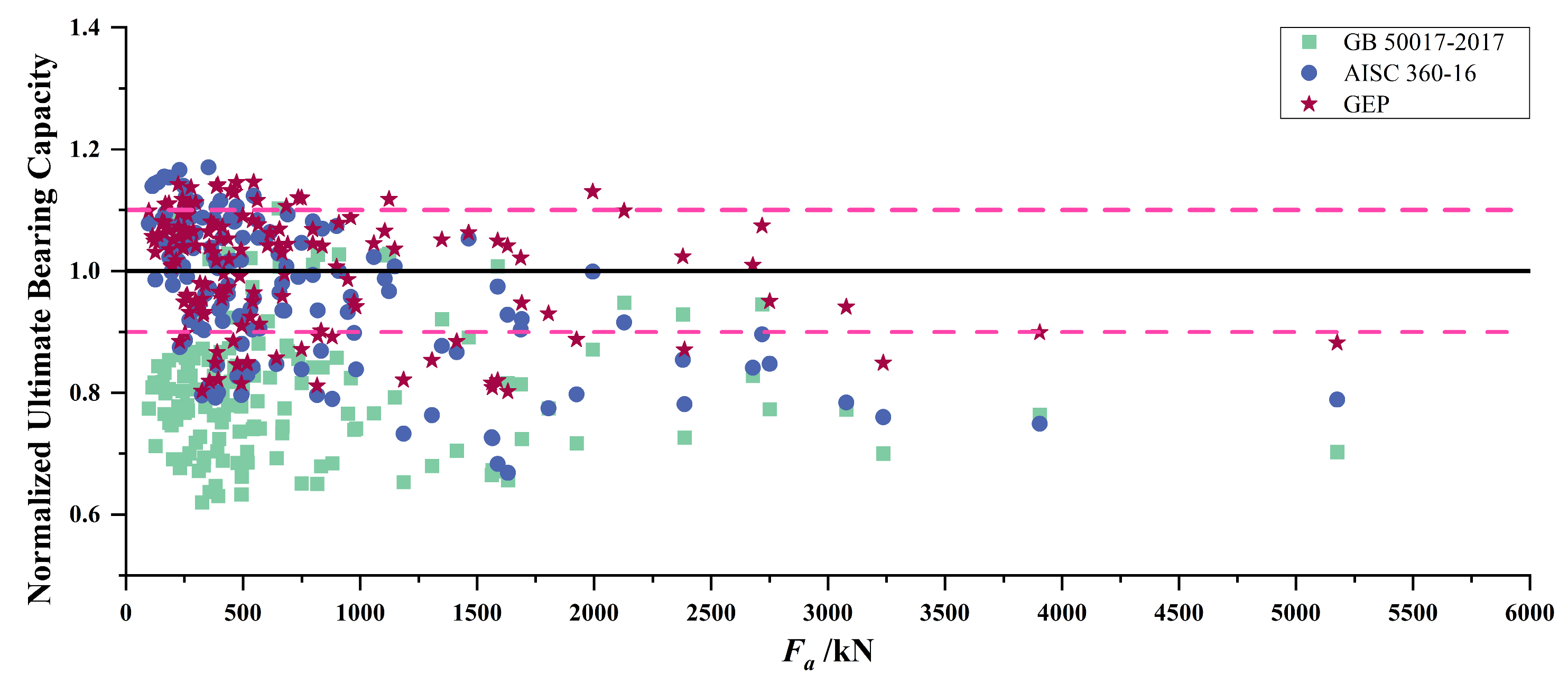
4.3. Validation and Analysis of the GEP Model

  • American specification
ANSI/AISC360-16 [34] provides the calculation method, as shown in Equations (28) and (29):
P d / P c + 8 M d / 9 M c = 1 , P d / P c 0.2
P d / 2 P c + M d / M c = 1 , P d / P c < 0.2
where Pd is the design strength, Pc is the available axial strength, Mc is the available flexural strength, and Md is the required flexural strength.
2.
Chinese specification
GB 50017-2017 [35] provides the calculation method, as shown in Equation (30):
P d / ( φ x A f ) + β m x M x / γ x W 1 x 1 0.8 P d / N E x f = 1
where Pd is the design strength, Mx is the end moment, N’Ex is the Euler critical load, γx is the plastic development coefficient of the cross-section, W1x is the elastic section modulus of the cross-section, and f is the design strength. Four types of column buckling curves are provided to estimate the stability coefficients (φx) of different column sections.
The GEP is compared with the calculation results of the three specifications, as shown in Figure 14. The vertical coordinate is the normalized ultimate bearing capacity, which is the ratio of each specification’s calculation result, the GEP calculation result, and the fiber model result (FGB/Fa, FAISC/Fa, FGEP/Fa). The black line represents a ratio of 1, while the pink dotted line represents an error of 10%. The horizontal coordinate is the ultimate bearing capacity, which is the result of the fiber model (Fa). The statistical parameters of various models, including R2, RMSE, and RAE, are presented in Table 9.
The results indicate that the ultimate bearing capacity calculated by the specifications is very conservative, because the current design specifications do not consider the unique material characteristics of cold-formed thick-walled profiles in component strength design. The analysis revealed that the estimation results of GEP, the American specification, and the Chinese specification decreased in order. The Chinese specification is the most conservative, while other specifications predict larger bearing capacities. Usually, the Chinese specification uses the design strength f, which is 0.9 times the yield strength of the material. The American specification uses the critical stress fcr calculated by Euler’s formula, and in this dataset, the ratio of critical stress to yield strength is less than 0.9. Therefore, the Chinese specification uses a smaller member strength parameter than the other specifications, resulting in a more significant estimated resistance of the axial compression bending members and a more conservative ultimate load capacity.
The accuracy, efficiency, and versatility of the GEP model were verified on cold-formed thick-walled square steel columns under axial compression, by comparing the numerical results with test data from various scholars [5,36]. Table 7 lists the specimen parameters and compares the experimental and fiber model analysis ultimate capacities, where B (mm) is the width of the cross-section, H (mm) is the height of the cross-section, R (mm) is the radius of the corner, δ0 (mm) is the geometric imperfection, Fu (kN) is the experimental ultimate load, and Fa (kN) and FGEP (kN) are the ultimate load calculated by the fiber model and GEP, respectively. It is worth noting that the possible reason for the large errors in some data is that some parameters of the experimental components exceed the range of the training set. The average FGEP-to-Fu and Fa-to-Fu ratios are 0.97 and 1.02, respectively. The main reason for this is that the column experiences local buckling at the mid-height due to its large width-to-thickness ratio. Therefore, within the error range, it can be considered that the GEP model is accurate.

5. Conclusions

In this paper, the main aim was to predict the ultimate load capacity of different members by using GEP and comparing it with the specifications. The results of the GEP calculation were compared with the traditional experimental test values or FEA results to determine whether the calculation was correct. The following conclusions can be drawn:
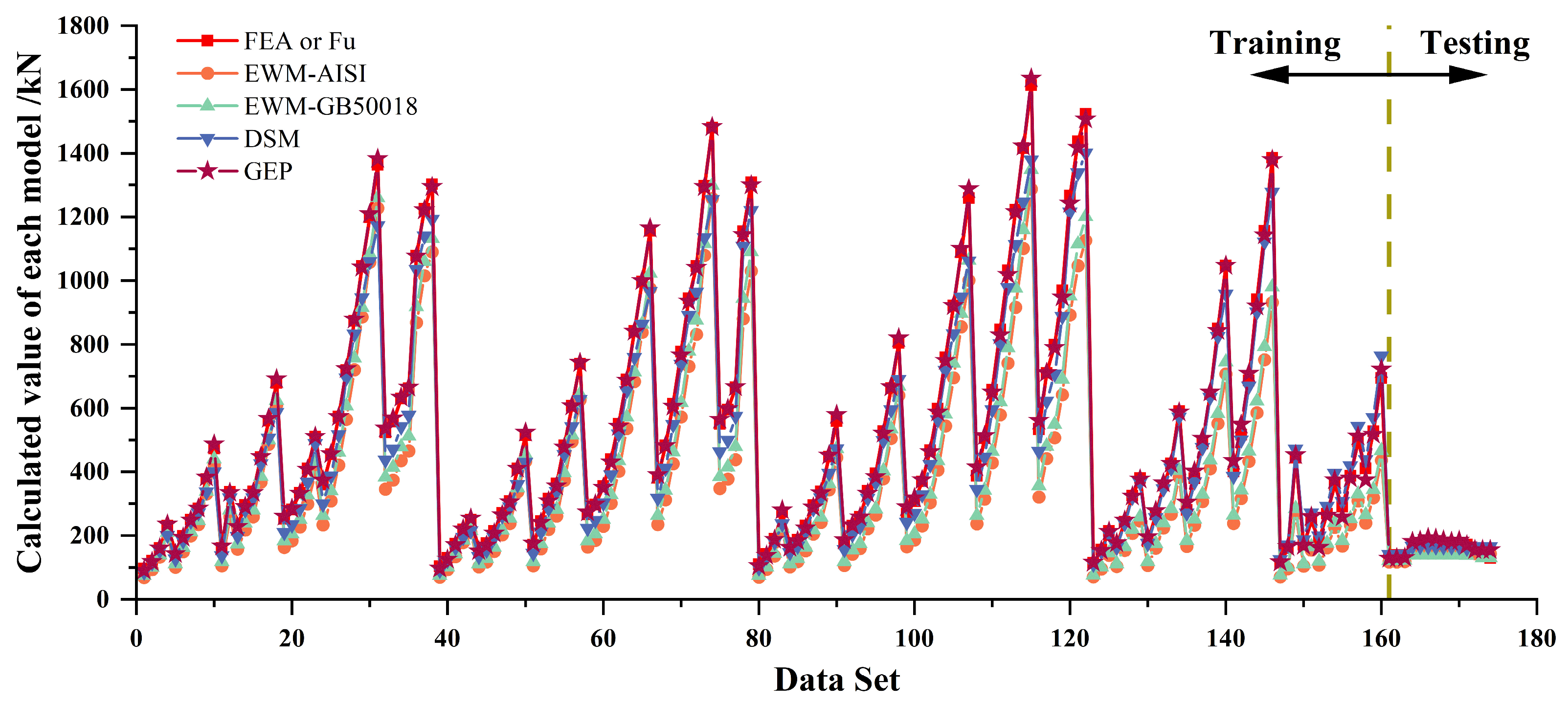
  • The study of the buckling resistance of BCF thin-walled tube columns under axial compression illustrates that the GEP model does not need to consider too many influencing factors (e.g., correlated buckling and elastic critical stress) to avoid excessive second-order errors. Comparing the results calculated by formulae based on GEP with the EWM and DSM calculation results on the test set, we found that the average value of the EWM is about 0.75, and that of the DSM is 0.92, while the average value and R2 of the results calculated using the GEP model exceed 0.95.
  • The study of the buckling resistance of cold-formed thick-walled steel columns under combined axial compression and bending illustrates that GEP can be used to construct a mechanical model similar to the existing specifications through an artificially specified mechanical model form. Comparing the results calculated by formulae based on GEP with the experimental data revealed that the average value was 1.007, with an R2 of 0.986.
  • All R2 values were greater than 0.95, indicating satisfactory accuracy in predicting the ultimate bearing capacity, and the comparison shows that GEP performs better than the existing design methods.
  • GEP performs better in predicting the ultimate load capacity of steel members, which solves the problem that the theoretical model cannot fully reflect the real situation of new steel structural members.

Author Contributions

Conceptualization, S.L. and W.K.; Methodology, W.K.; Software, S.L.; Writing—Original Draft Preparation, S.L.; Writing—Review and Editing, S.L.; Project Administration, W.K. All authors have read and agreed to the published version of the manuscript.

Funding

The authors are grateful for the financial support of the Research Project of China Railway Construction Group Co., Ltd. (No. 23-01a).

Data Availability Statement

The original contributions presented in the study are included in the article, further inquiries can be directed to the corresponding author.

Conflicts of Interest

The authors declare that this study received funding from China Railway Construction Group Co., Ltd., East China Engineering Co., Ltd. The funder was not involved in the study design, collection, analysis, interpretation of data, the writing of this article or the decision to submit it for publication.

References

  1. AISI S100; North American Specification for the Design of Cold-Formed Steel Structural Members. American Iron and Steel Institute: Washington, DC, USA, 2016.
  2. AS/NZS 4600; Cold-Formed Steel Structures. Australian/New Zealand Standard: Sydney, Australia, 2018.
  3. Stone, T.A.; LaBoube, R.A. Behavior of cold-formed steel built-up I-sections. Thin-Walled Struct. 2005, 43, 1805–1817. [Google Scholar] [CrossRef]
  4. Roy, K.; Ting TC, H.; Lau, H.H.; Lim, J.B. Effect of thickness on the behaviour of axially loaded back-to-back cold-formed steel built-up channel sections-Experimental and numerical investigation. Structures 2018, 16, 327–346. [Google Scholar] [CrossRef]
  5. Hou, G. Experimental Research and Numerical Analysis on Axial Compression Performance of Cold-Formed Non-Thin-Walled Square Hollow Sections; Tongji University: Shanghai, China, 2011. (In Chinese) [Google Scholar]
  6. Liu, Z.; Liu, H.; Chen, Z.; Zhang, G. Structural behavior of cold-formed thick-walled rectangular steel columns. J. Constr. Steel Res. 2018, 147, 277–292. [Google Scholar] [CrossRef]
  7. Tong, L.; Hou, G.; Chen, Y.; Zhou, F.; Shen, K.; Yang, A. Experimental investigation on longitudinal residual stresses for cold-formed thick-walled square hollow sections. J. Constr. Steel Res. 2012, 73, 105–116. [Google Scholar] [CrossRef]
  8. Tenpe, A.R.; Patel, A. Application of genetic expression programming and artificial neural network for prediction of CBR. Road Mater. Pavement Des. 2020, 21, 1183–1200. [Google Scholar] [CrossRef]
  9. D’Aniello, M.; Güneyisi, E.M.; Landolfo, R.; Mermerdaş, K. Analytical prediction of available rotation capacity of cold-formed rectangular and square hollow section beams. Thin-Walled Struct. 2014, 77, 141–152. [Google Scholar] [CrossRef]
  10. Cevik, A. A new formulation for web crippling strength of cold-formed steel sheeting using genetic programming. J. Constr. Steel Res. 2007, 63, 867–883. [Google Scholar] [CrossRef]
  11. Momeni, M.; Hadianfard, M.A.; Bedon, C.; Baghlani, A. Damage evaluation of H-section steel columns under impulsive blast loads via gene expression programming. Eng. Struct. 2020, 219, 110909. [Google Scholar] [CrossRef]
  12. Ferreira, C. Gene expression programming: A new adaptive algorithm for solving problems. arXiv 2001, arXiv:cs/0102027. [Google Scholar]
  13. Zhang, X.D.; Li, J. Gene expression programming based on parallel tabu search for improving model accuracy. Appl. Mech. Mater. 2013, 411, 1930–1934. [Google Scholar] [CrossRef]
  14. Wang, M.; Wan, W. A new empirical formula for evaluating uniaxial compressive strength using the Schmidt hammer test. Int. J. Rock Mech. Min. Sci. 2019, 123, 104094. [Google Scholar] [CrossRef]
  15. Lu, Q.; Zhou, S.; Tao, F.; Luo, J.; Wang, Z. Enhancing gene expression programming based on space partition and jump for symbolic regression. Inf. Sci. 2021, 547, 553–567. [Google Scholar] [CrossRef]
  16. ABAQUS. User Manual, version 6.16; DS SIMULIA Corp.: Providence, RI, USA, 2021. [Google Scholar]
  17. Rokilan, M.; Mahendran, M. Elevated temperature mechanical properties of cold-rolled steel sheets and cold-formed steel sections. J. Constr. Steel Res. 2020, 167, 105851. [Google Scholar] [CrossRef]
  18. Schafer, B.W.; Peköz, T. Computational modeling of cold-formed steel: Characterizing geometric imperfections and residual stresses. J. Constr. Steel Res. 1998, 47, 193–210. [Google Scholar] [CrossRef]
  19. Kechidi, S.; Fratamico, D.C.; Schafer, B.W.; Castro, J.M.; Bourahla, N. Simulation of screw connected built-up cold-formed steel back-to-back lipped channels under axial compression. Eng. Struct. 2020, 206, 110109. [Google Scholar] [CrossRef]
  20. Nie, S.; Zhou, T.; Eatherton, M.R.; Li, J.; Zhang, Y. Compressive behavior of built-up double-box columns consisting of four cold-formed steel channels. Eng. Struct. 2020, 222, 111133. [Google Scholar] [CrossRef]
  21. Vy, S.T.; Mahendran, M.; Sivaprakasam, T. Built-up back-to-back cold-formed steel compression members failing by local and distortional buckling. Thin-Walled Struct. 2021, 159, 107224. [Google Scholar] [CrossRef]
  22. Fratamico, D.C.; Torabian, S.; Zhao, X.; Rasmussen, K.J.; Schafer, B.W. Experiments on the global buckling and collapse of built-up cold-formed steel columns. J. Constr. Steel Res. 2018, 144, 65–80. [Google Scholar] [CrossRef]
  23. GB 50205-2020; Standard for Acceptance of Construction Quality of Steel Structure. China Architecture & Building Press: Beijing, China, 2020. (In Chinese)
  24. Gardner, L.; Nethercot, D.A. Numerical modeling of stainless steel structural components—A consistent approach. J. Struct. Eng. 2004, 130, 1586–1601. [Google Scholar] [CrossRef]
  25. Lu, Y. Research on the Instability Mechanism and Bearing Capacity Design Method of Cold-Formed Thin-Walled Steel Double-Leg Split Axial Compression Columns; Changan University: Xi’an, China, 2018. (In Chinese) [Google Scholar]
  26. Ting, C.H.T. The Behaviour of Axially Loaded Cold-Formed Steel Back-to-Back C-Channel Built-Up Columns. Ph.D. Thesis, Curtin University, Bentley, Australia, 2013. [Google Scholar]
  27. Wang, Q. Experimental and Theoretical Research on Bearing Capacity of Cold-Formed Thin-Walled Steel Composite Columns with Open Double Legs; Changan University: Xi’an, China, 2009. (In Chinese) [Google Scholar]
  28. GB 50018-2002; Technical Code of Cold-Formed Thin-Wall Steel Structures. China Architecture & Building Press: Beijing, China, 2002. (In Chinese)
  29. Zhou, Y.; Huang, D.; Li, T.; Li, Y. Buckling resistance of cold-formed thick-walled steel columns under combined axial compression and bending. J. Build. Eng. 2022, 51, 104300. [Google Scholar] [CrossRef]
  30. Shen, Z.Y.; Wen, D.H.; Li, Y.Q.; Ma, Y. Distribution patterns of material properties for cross-section of cold-formed thick-walled steel rectangular tubes. J. Tongji Univ. (Nat. Sci.) 2016, 44, 981–990. (In Chinese) [Google Scholar]
  31. Wang, L.P. Experimental Investigation on Cold-Forming Effect of Thick-Walled Steel Sections; Tongji University: Shanghai, China, 2011. (In Chinese) [Google Scholar]
  32. Zhu, A.Z. Experimental Investigation of Cold-Formed Effect on Thick-Walled Steel Members and Analysis of the Cold-Formed Residual Stress Field. Master’s Thesis, Wuhan University, Wuhan, China, 2004. (In Chinese). [Google Scholar]
  33. Liu, D.; Liu, H.; Chen, Z.; Liao, X. Structural behavior of extreme thick-walled cold-formed square steel columns. J. Constr. Steel Res. 2017, 128, 371–379. [Google Scholar] [CrossRef]
  34. ANSI/AISC 360-16; Specification for Structural Steel Buildings. American Institute of Steel Construction (AISC): Chicago, IL, USA, 2016.
  35. GB 50017-2017; Standard for Design of Steel Structures. China Architecture & Building Press: Beijing, China, 2017. (In Chinese)
  36. Li, G.W.; Li, Y.Q. Overall stability behavior of axially compressed cold-formed thick-walled steel tubes. Thin-Walled Struct. 2018, 125, 234–244. [Google Scholar] [CrossRef]
Figure 1. Two expressions of GEP.
Buildings 15 01597 g001
Figure 2. Algorithm flowchart of GEP.
Buildings 15 01597 g002
Figure 3. Finite element model.
Buildings 15 01597 g003
Figure 4. Different modeling methods for bolts [21].
Buildings 15 01597 g004
Figure 5. Analysis of mesh sensitivity [21].
Buildings 15 01597 g005
Figure 6. Finite element model validation [25].
Buildings 15 01597 g006
Figure 7. Model for parameter research.
Buildings 15 01597 g007
Figure 8. Parametric analysis.
Buildings 15 01597 g008
Figure 9. Expression tree of BCF thin-walled columns.
Buildings 15 01597 g009
Figure 10. Evaluation of various models.
Buildings 15 01597 g010
Figure 11. Flowchart for fiber model.
Buildings 15 01597 g011
Figure 12. Parametric analysis.
Buildings 15 01597 g012
Figure 13. The best expression tree of cold-formed thick-walled steel columns.
Buildings 15 01597 g013
Figure 14. Evaluation of various models.
Buildings 15 01597 g014
Table 1. General parameter settings of GEP.
Parameter Setting
GeneralChromosomes30
Fitness functionEquation (2)
Genetic operatorsMutation rate0.044
Inversion rate0.1
IS transposition rate0.1
RIS transposition rate0.1
Gene transposition rate0.1
One-point recombination rate0.3
Two-point recombination rate0.3
Gene recombination rate0.1
Random numerical constantRNC mutation0.00206
DC mutation0.00206
DC inversion0.00546
DC IS transposition0.00546
Constants per gene10
Data typeFloating-point
Value range−10–10
Table 2. Error of different simulation methods for bolts.
2S-150 [20]SolidCouplingFastenerSpring
Load (kN)94.8899.7997.9197.6297.75
Error/5.1%3.1%2.9%3%
Table 3. Key parameters of columns for parametric studies.
ParametersValue
Web height (h/mm)90, 120, 150, 180, 210, 240
Single-member flange width (b/mm)0.33 h, 0.4 h, 0.5 h, 0.67 h, h
Lip width (d/mm)0.5 b
Thickness (t/mm)1, 1.2, 1.5, 2, 2.5, 3, 3.5, 4, 4.5, 5
Initial geometric imperfectionsb/100
Bolt transverse distance (e)h/2
Bolt position along the length direction0.25 L, 0.5 L, 0.75 L
Table 4. Parameters used as inputs, and their target values.
TypeParametersMinimumMaximum
InputCalculated length (L/mm)108288
InputSingle-member flange width (b/mm)30210
Lip width (d/mm)1540
InputWeb height (h/mm)90240
InputThickness (t/mm)15
InputOutside diameter of rounded corner (R/mm)210
Initial geometric imperfection (Im/mm)0.32.1
Elastic modulus (E/GPa)216216
InputYield strength (fy/MPa)235235
InputTotal area (A/mm2)3524773.12
OutputUltimate bearing capacity (FEA/kN)96.381613.7
Table 5. Statistical performance of different models in the training and testing sets.
ModelR2RMSERAEAverageSD
EWM-TrainGB50018-20200.978143.130.4110.7540.051
AISI S100 20160.973171.900.4990.7030.063
DSM-Train0.99067.130.1690.9230.069
GEP-Train1.00011.440.0290.9990.031
EWM-TestGB50018-20020.72347.221.7430.7330.108
AISI S100 20160.74342.121.5270.7830.129
DSM-Test0.82313.350.4170.9670.100
GEP-Test0.95111.490.2660.9770.073
Table 6. Comparison between experimental and numerical capacities of bolted built-up H-section columns.
SourceSpecimenLbdhtRImEfyAFuFGEPFGEP/Fu
[25]SC3-140-A145143.214.5143.51.482.40.4205305.4748.82130.7128.710.98
SC3-140-A245142.814.9144.41.482.40.4205305.4751.48139.6129.960.93
SC3-140-A345143.415.3143.11.482.40.4205305.4753.56138.8130.400.94
[26]90S50L300-127749.814.691.31.21.50.5205.72557.5516.72172.5180.721.05
90S50L300-227249.714.591.81.21.50.5205.72557.5516.96171.6184.311.08
90S50L300-326149.414.592.91.21.50.5205.72557.5518.16167.6192.801.15
90S100L300-326249.714.690.81.21.50.5205.72557.5515.04171.2189.931.11
90S100L300-426849.514.690.61.21.50.5205.72557.5513.6173.9184.951.06
90S200L300-1273.549.414.690.71.21.50.5205.72557.5513.36170.3181.081.06
90S200L300-2269.549.414.690.71.21.50.5205.72557.5513.36177.5183.811.03
90S200L300-4280.548.31489.51.21.50.5205.72557.5502.32171.9169.640.99
[27]DC450-145041141401.62.40.4223334.04779.52160154.090.96
DC450-245041141401.62.40.4223334.04779.52150154.091.03
DC450-345041141401.62.40.4223334.04779.52130154.091.18
Table 7. Comparison between experimental and numerical capacities of cold-formed thick-walled steel columns.
SpecimenBHRtfyEGradeLδ0FuFaFa/FuFGEPFGEP/Fu
S108 × 108 × 10-110810820.510.1511199Q34536201.348307360.89787.60.949
S108 × 108 × 10-210810820.510.1511199Q345362018547450.87787.60.922
S135 × 135 × 10-113513521.610391206Q34534953.6112011481.031271.11.135
S135 × 135 × 10-213513521.610391206Q34534954.15106511331.061271.11.194
R400 × 200 × 10-140020024.110368204Q34533454.24340534881.023747.91.101
R400 × 200 × 10-240020024.110368204Q34533454.41334034791.043747.91.122
S250 × 250 × 8-125025022.37.9395197Q34529402243927391.122587.51.061
S250 × 250 × 8-225025022.37.9395197Q34529407.7227525721.132587.51.137
S140 × 140 × 10-11401402510406206Q34531101.36146314450.991430.60.978
S140 × 140 × 10-21401402510406206Q34541501.82113010920.971191.71.055
S200 × 200 × 12-12002003612368206Q23527301.3268827401.022009.90.748
S200 × 200 × 12-22002003612368206Q23534801.66247825641.041937.50.782
S200 × 200 × 12-32002003612368206Q23541601.98223323591.061859.80.833
S200 × 200 × 16-12002004816453206Q34526501.24404043831.093660.80.906
S200 × 200 × 16-22002004816453206Q34533801.59387539971.033477.00.897
S200 × 200 × 16-32002004816453206Q34541101.93363035790.993261.40.898
S150 × 150 × 8-1150150208503206Q34522951.1196418530.941443.20.735
S150 × 150 × 8-2150150208503206Q34531501.51142815161.061310.50.918
S150 × 150 × 8-3150150208503206Q34540051.92114011701.031154.51.013
Table 8. Parameters used as inputs, and their target values.
TypeParametersMinimumMaximum
InputThe long edge (a/mm)86350
Outside diameter of rounded corner (R/mm)2048
Thickness (t/mm)816
Elastic modulus (E/GPa)204204
InputAverage strength (fa/MPa)281552.21
InputYield strength (fy/MPa)235345
InputTotal area (A/mm2)2276.2420,277.24
InputCalculated length (L/mm)608.2527,218.23
InputSlenderness ratio (λ)17.01204.03
InputPlastic section modulus (W/mm3)73,2642,679,394
InputEccentricity (e/mm)0850.76
OutputUltimate bearing capacity (Fa/kN)64.057702.96
Table 9. Statistical parameters of various models.
ModelR2RMSERAEAverageSD
AISC 360-160.978206.050.1710.9670.117
GB 50017-20170.970245.670.2690.8230.101
GEP0.986124.470.1361.0070.092
Disclaimer/Publisher’s Note: The statements, opinions and data contained in all publications are solely those of the individual author(s) and contributor(s) and not of MDPI and/or the editor(s). MDPI and/or the editor(s) disclaim responsibility for any injury to people or property resulting from any ideas, methods, instructions or products referred to in the content.

