Analysis and Prediction of Deformation of Shield Tunnel Under the Influence of Random Damages Based on Deep Learning

Abstract

Shield tunnels in operation are often affected by complex geological conditions, environmental factors, and structural aging, leading to cumulative damage in the segments and, consequently, increased deformation that compromises structural safety. To investigate the deformation behavior of tunnel linings under random damage conditions, this study integrates finite element numerical simulation with deep learning techniques to analyze and predict the deformation of shield tunnel segments. First, a refined three-dimensional finite element model was established, and a random damage modeling method was developed to simulate the deformation evolution of tunnel segments under different damage ratios. Additionally, a statistical analysis was conducted to assess the uncertainty in deformation caused by random damage. Furthermore, this study introduces a convolutional neural network (CNN) surrogate model to enable the rapid prediction of shield tunnel deformation under random damage conditions. The results indicate that as the damage ratio increases, both the mean deformation and its variability progressively rise, leading to increased deformation instability, demonstrating the cumulative effect of damage on segment deformation. Moreover, the 1D-CNN surrogate model was trained using finite element computation results, and predictions on the test dataset showed excellent agreement with FEM calculations. The surrogate model achieved a correlation coefficient (R²) exceeding 0.95 and an RMSE below 0.016 mm, confirming its ability to accurately predict the deformation of tunnel segments across different damage conditions. To the best of our knowledge, the finite-element–deep-learning hybrid approach proposed in this study provides a valuable theoretical foundation for predicting the deformation of in-service shield tunnels and assessing structural safety, offering scientific guidance for tunnel safety evaluation and damage repair strategies.

1. Introduction

With the rapid expansion of urban underground space utilization, shield tunneling methods have become the dominant construction method for metro systems and utility tunnels due to their high efficiency and minimal environmental impact [1,2,3,4,5,6,7]. However, under complex geological conditions—such as soft soil layers, high groundwater levels, and disturbances from adjacent construction activities—shield tunnel segments are prone to various structural deteriorations [8,9,10]. These include concrete carbonation, steel corrosion, structural cracking, and spalling, all of which gradually reduce the stiffness of the tunnel lining and exacerbate transverse deformation. This degradation process may trigger joint leakage, crack propagation, and ultimately, global instability [11,12,13,14], posing significant threats to operational safety. Consequently, investigating and predicting the deformation characteristics and evolutionary patterns of shield tunnels affected by existing structural deterioration is a critical scientific challenge in ensuring their long-term service performance.

Unraveling the mechanisms of tunnel deterioration evolution and analyzing the impact of existing defects on segment deformation and load-bearing capacity serve as the foundation for ensuring shield tunnel safety. To address these challenges, numerous scholars have conducted extensive research employing various technological approaches, focusing on damage monitoring, evolution patterns, and remediation strategies [15,16,17]. Park [18] proposed a Python-based TOUGH-FLAC (5.01) simulation method to investigate the impact of water leakage on tunnel linings and surrounding strata. The study found that an increase in leakage volume not only exacerbates surface settlement but also enhances tunnel instability. Additionally, the influence of leakage location and quantity on tunnel structures was analyzed. Zheng et al. [19] developed a mechanical analytical model for fault-crossing tunnels. The study revealed that fault dislocation induces changes in the longitudinal internal forces of the tunnel, posing a threat to the structural safety of the tunnel.

With the rapid advancement of artificial intelligence, its application in tunnel engineering has yielded promising results [20,21,22,23,24]. For instance, Feng et al. [25] proposed a deep-learning-based method for the rapid and automatic identification of tunnel lining leakage, enabling precise image segmentation and the quantitative evaluation of leakage conditions. Yu et al. [26] developed a deep neural network architecture combining YOLOv5 and JLNet to accurately extract longitudinal joint opening in shield tunnels, demonstrating high prediction accuracy. Similarly, Wang et al. [27] introduced a physics-informed neural network (PINN) to predict railway subgrade settlements induced by shield tunneling, proving its superiority over traditional methods. Zhao et al. [28] developed a mask-guided regional hybrid attention convolutional neural network (Mask R-HACNN) and a mesoscale cohesive numerical model to investigate the mechanical behavior of segments and joints during crack damage evolution. These studies collectively highlight the advantages of machine learning methods over traditional approaches, such as experiments and finite element analysis, in certain aspects of tunnel engineering, demonstrating their superior computational efficiency and effectiveness.

Due to the complexity of the underground environment and the multi-phase nature of concrete, cracking and damage in shield tunnels often exhibit a random distribution [29,30,31]. Previous studies have not considered the influence of random damage on the deformation of shield segments. Moreover, given the high computational cost of numerical simulations and physical experiments, obtaining a rapid understanding of deformation behavior under various damage scenarios remains a significant challenge [32,33,34]. In addition, although numerous studies have focused on engineering problems during the construction phase [35,36,37,38], research on structural damage and deformation in operational tunnels remains relatively limited. Therefore, it is essential to study the influence of random damage on the deformation of shield segments and to develop new methodologies to efficiently predict the deformation of shield tunnels subjected to random damage.

To address this issue, this study developed a detailed 3D finite element numerical model to analyze the impact of random damage on the transverse deformation of an in-service shield tunnel. A dataset of 2000 deformation samples was generated for different damage proportions in shield segments. Statistical analyses were then performed on the transverse and vertical convergence values to quantify the influence of random segment damage on transverse convergence. Additionally, a one-dimensional convolutional neural network (1D-CNN) surrogate model was designed to predict segment deformation.

2. Numerical Simulation

2.1. Numerical Model

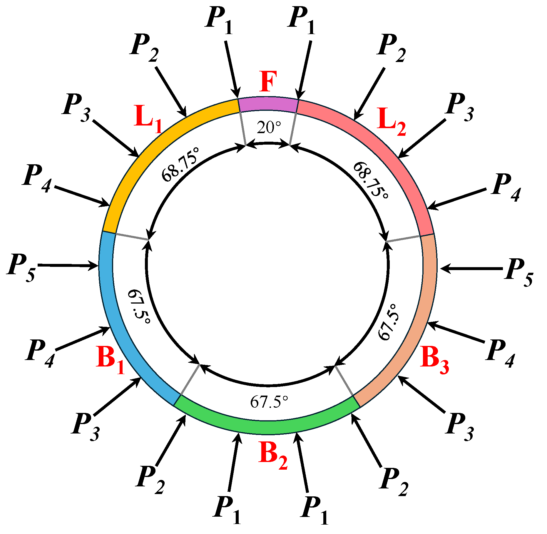
Wei et al. [39] designed and conducted a full-scale loading test to study the failure characteristics of shield segments under loading, and to document the deformation process of the segments under an external load in detail. To validate the numerical model, the model used in this study was designed to match the structural configuration and dimensions of the experimental setup. Figure 1 illustrates the segment arrangement and the load distribution applied in the shield tunnel test. The precast concrete segments were geometrically defined with an outer diameter of 6.2 m, an inner diameter of 5.5 m, a wall thickness of 0.35 m, and a longitudinal width of 1.2 m. Each annular lining ring adopted a six-segment assembly configuration, consisting of three functionally differentiated types: one radially constrained capping segment spanning a 20° central angle (block F), two adjacent segments each occupying a 68.75° central angle (block L₁ and block L₂), and three standard segments with identical 67.5° central angles (block B₁, block B₂, and block B₃).

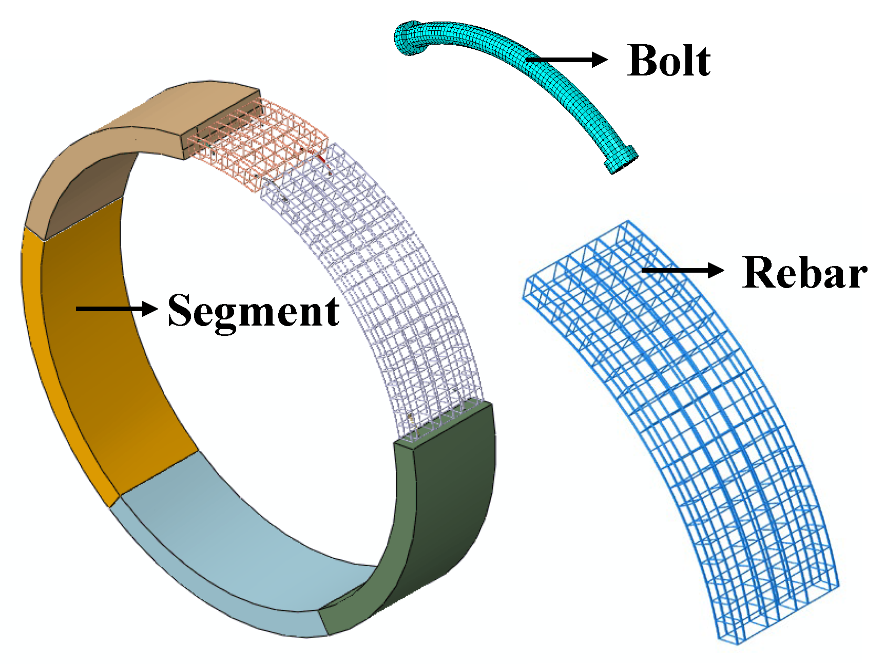
This study establishes a refined numerical model of a single-ring shield tunnel segment, which primarily includes key structural components such as the tunnel segment, bent bolts, nuts, and the reinforcement cage, as shown in Figure 2. The reinforcement cage in the model consists of longitudinal reinforcement bars and stirrups to more accurately reflect the mechanical behavior of the segment. Given the structural complexity of the shield tunnel and the need for extensive parametric analysis in this study, a fully detailed geometric model would result in excessive computational costs and potential convergence issues. Therefore, based on existing research experience, appropriate simplification has been applied. Specifically, detailed features such as waterproof grooves and gaskets were omitted in the finite element model to improve computational efficiency while preserving key mechanical characteristics [34,39]. Regarding element selection, the shield tunnel segment and bent bolts were modeled using C3D8R elements (eight-node reduced-integration 3D solid elements) to ensure computational accuracy and stability, while the reinforcement cage was modeled using T3D3 elements (three-node 3D truss elements) to effectively capture the reinforcement behavior. The final shield tunnel segment model consisted of 10,816 finite elements.

2.2. Constitutive and Parameters of the Model

In this study, the reduction of Young’s modulus was randomly applied to simulate the stiffness degradation of concrete due to cracking, corrosion, or other damage mechanisms. Consequently, the concrete was modeled using an elastic constitutive model, while the reinforcement bars and bolts were represented by a bilinear elastoplastic constitutive model to better capture their mechanical behavior. The concrete was classified as C55 grade, with a Young’s modulus of 34.5 GPa and a Poisson’s ratio of 0.3. The reinforcement bars were HRB400-grade, while the bent bolts are 8.8-grade high-strength bolts.

The interaction between reinforcement and concrete was modeled using an embedded constraint, while the contact between segments and between segments and bolts was defined using a surface-to-surface contact model. The normal contact behavior followed a hard contact approach, whereas the tangential behavior was governed by the penalty method, with friction coefficients set to 0.5 for segment-to-segment interactions and 0.3 for segment-to-bolt interactions. This contact formulation allows for joint opening, misalignment, and sliding but prevents interpenetration. The surface-to-surface contact model effectively captures the interaction between shield tunnel segments, ensuring higher computational accuracy and reliability in structural response predictions.

2.3. Loading Procedure

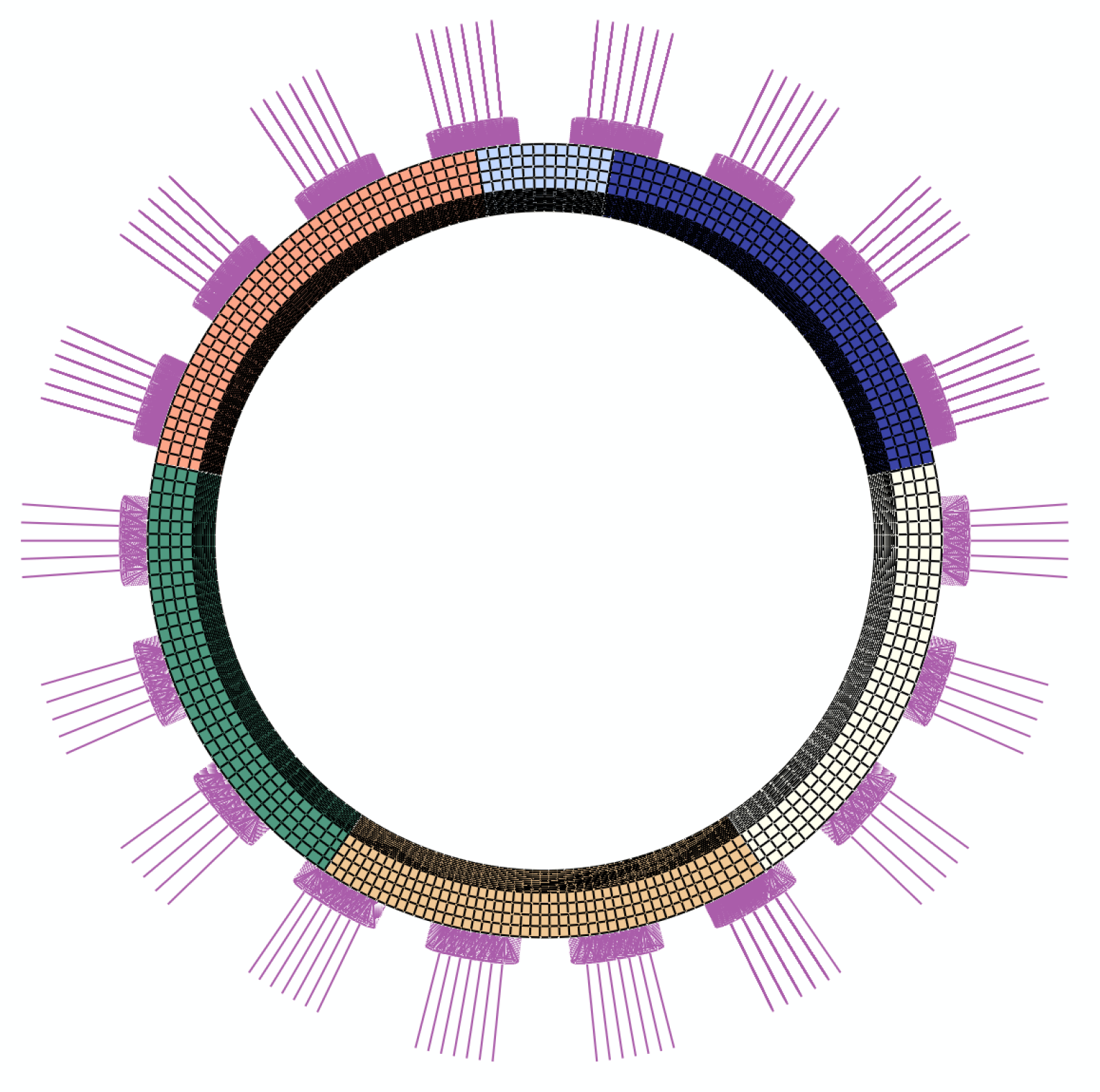
As shown in Figure 3, the loading scheme in the numerical simulation follows the same 18-point loading method as in the full-scale test. According to Wei et al. [39], the applied forces are symmetric in both horizontal and vertical directions, meaning that only five distinct force magnitudes exist, as illustrated in Figure 1. These forces are denoted as P₁ to P₅, where P₁ represents the load at the crown, and P₅ corresponds to the load at the haunch. Given the complexity of the force distribution between the crown and haunch, a simplified assumption is made in which the load varies linearly across this region.

All forces are computed based on P₁, which increases from 0 to its design value, while P₅ remains 0.6 times P₁ (i.e., lateral earth pressure coefficient a = 0.6). The intermediate forces P₂, P₃, and P₄ are determined using the following equations: P₂ = P₅ + 3 × (P₁ − P₅)/4, P₃ = P₅ + (P₁ − P₅)/2, and P₄ = P₅ + (P₁ − P₅)/4. In this study, the natural unit weight of the soil is set to 18 kN/m³, and the tunnel crown depth is 15 m. Based on the above equations, the calculated values are as follows: P₁ = 270 kN, P₂ = 243 kN, P₃ = 216 kN, P₄ = 189 kN, P₅ = 162 kN.

2.4. Model Verification

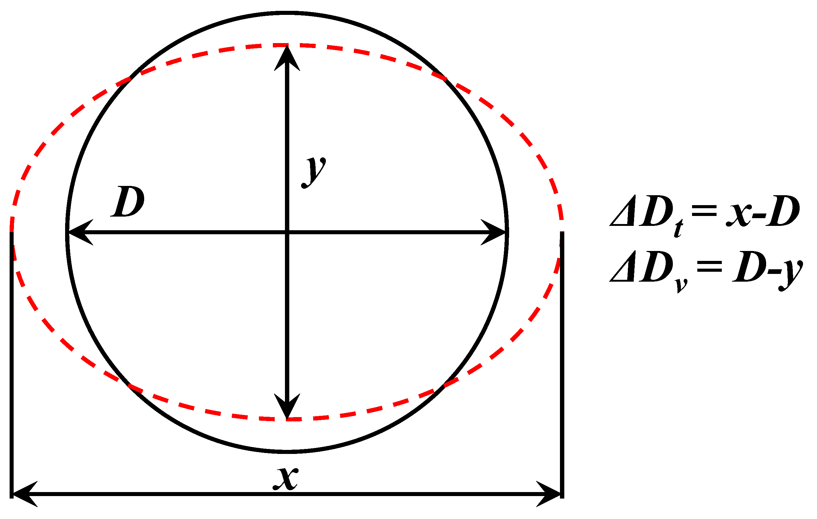
The deformation mode of the shield segment under loading is illustrated in Figure 4. As the segment deforms, its shape gradually transitions from a circular to an elliptical form. Here, D represents the initial internal diameter of the shield tunnel, while x denotes the major axis of the ellipse after deformation. In this study, the transverse convergence of the segment (ΔDt) is defined as the constant positive difference between x and D after deformation, expressed as ΔD_t = x − D. Similarly, the vertical displacement of the segment (ΔD_v) is quantified as the difference in vertical deformation, given by ΔD_v = D − y, where y represents the minor axis of the deformed ellipse.

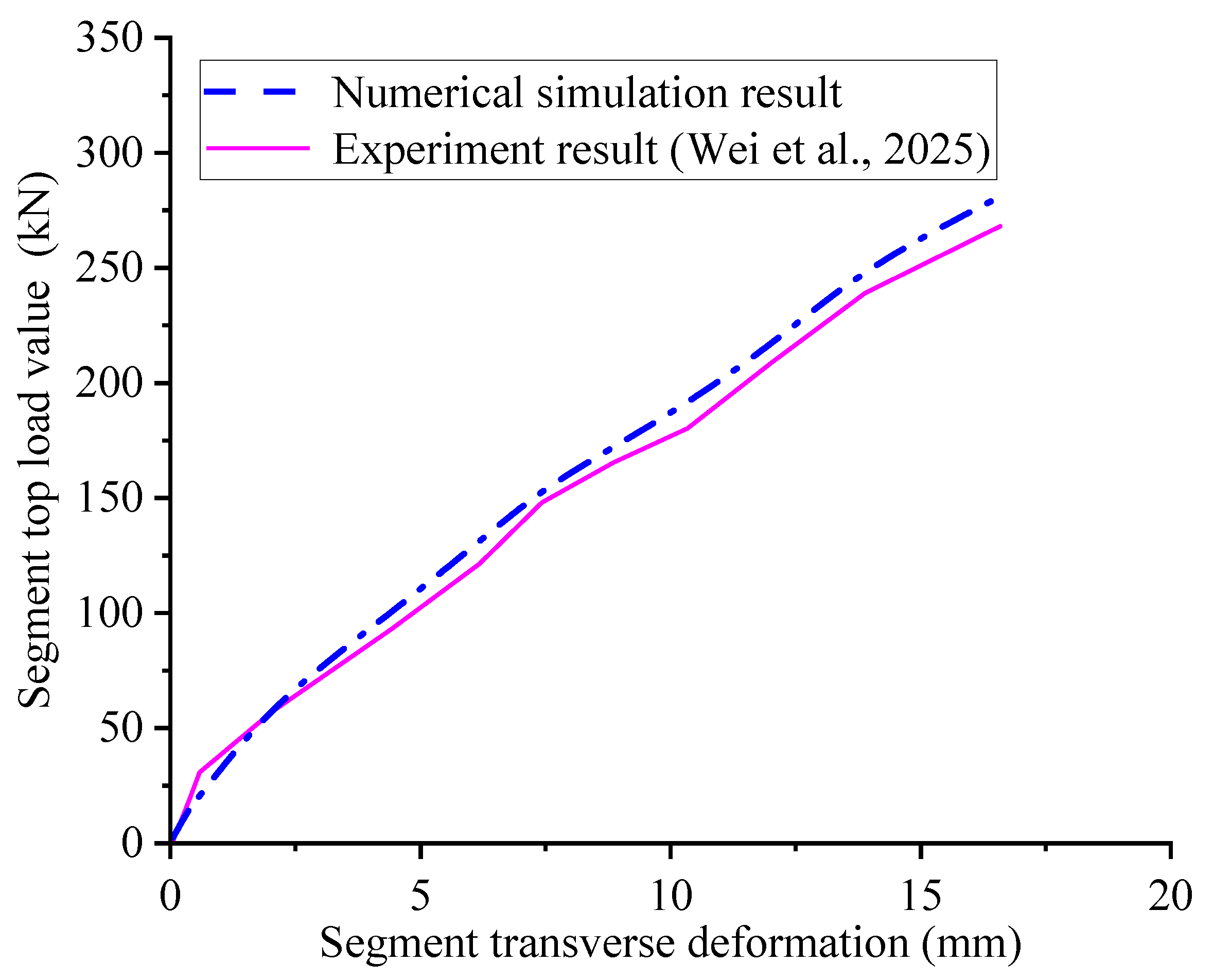
To validate the accuracy of the proposed model and computational approach, a comparative analysis was performed between the finite element method (FEM) results and full-scale experimental data, focusing on the transverse deformation of an intact shield segment under an increasing crown load P₁. As shown in Figure 5, the comparison demonstrates that when the applied load reaches the assumed burial depth, the deformation curve obtained from numerical simulation closely aligns with the observed trend in the full-scale test. The maximum discrepancy between the two results is within 3%, indicating that the numerical modeling approach employed in this study is both accurate and reliable.

2.5. Realization of Random Damage of Shield Segment

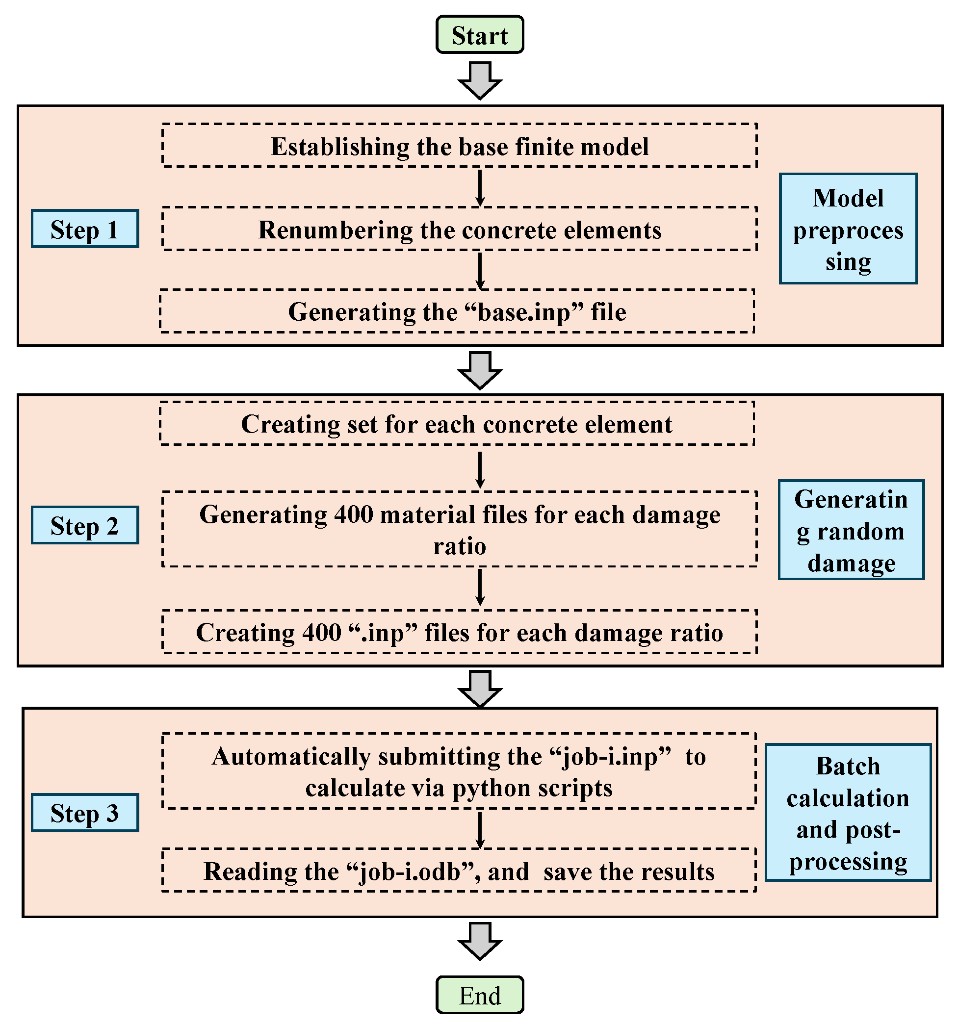
Abaqus does not provide built-in functionality for automatic random damage modeling of shield tunnel segments, nor does it support batch processing and automated result extraction. To address these limitations, this study integrated MATLAB 2023b, Python 3.12, and Abaqus 2022 to develop a program that enables random damage modeling, automated computation, and result extraction for shield tunnel segments. As shown in Figure 6, the implementation process is as follows:

(1) According to the keyword syntax rules of Abaqus “.inp” files, the mesh elements of the tunnel segment are renumbered to allow for the random selection of damaged elements (by default, Abaqus numbers each part of the grid individually). And each concrete grid element is assigned an individual set, ensuring that unique material properties and section parameters can be allocated.

(2) The damage ratio is predefined, and as an example, a damage ratio of 0.1 (i.e., 10% of the concrete elements were damaged) is considered. Among 10,816 concrete grid elements, 10% are randomly selected, and their Young’s modulus is randomly reduced between 10% and 90% of the original value (to prevent computational errors, the lower limit is set to 10% instead of zero). Based on the “base.inp” file, the material properties and section parameters of the selected elements are modified to generate the corresponding “job-i.inp” file. For each damage ratio, 400 different computational models are generated.

(3) Since Abaqus allows flexible pre-processing and post-processing using Python, a Python script was developed to automate the entire computation process. The script iteratively submits the simulation jobs for each damage ratio, and once the computations are complete, it automatically opens the “job-i.odb” files, extracts the required results, and saves them until all simulations are finalized.

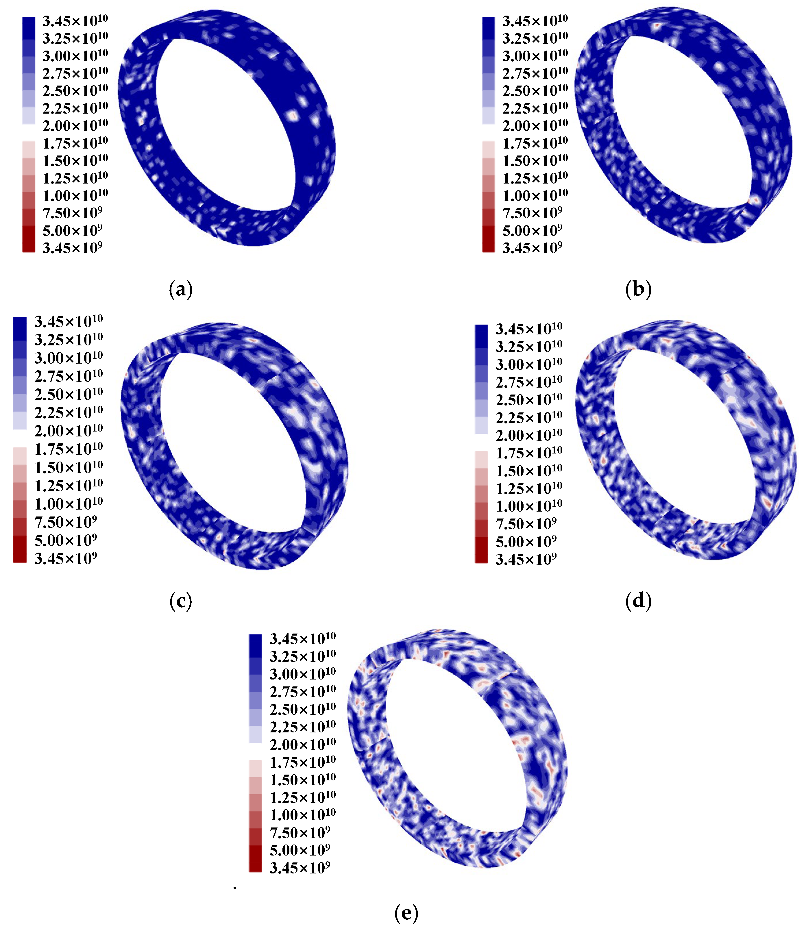
By following the aforementioned steps, random damage modeling and the automated computation of shield tunnel segments can be successfully achieved. Figure 7 illustrates typical implementations under different damage ratios. As shown in Figure 7, the proposed method effectively simulates the random damage of tunnel segments. With an increasing damage ratio, the number of damaged elements progressively rises, exhibiting a completely random distribution. This demonstrates the effectiveness of the method in accurately modeling stochastic damage patterns.

Figure 6. Random damage realization of shield segment and calculation process.

Figure 6. Random damage realization of shield segment and calculation process.

3. Deformation Analysis of Shield Segment

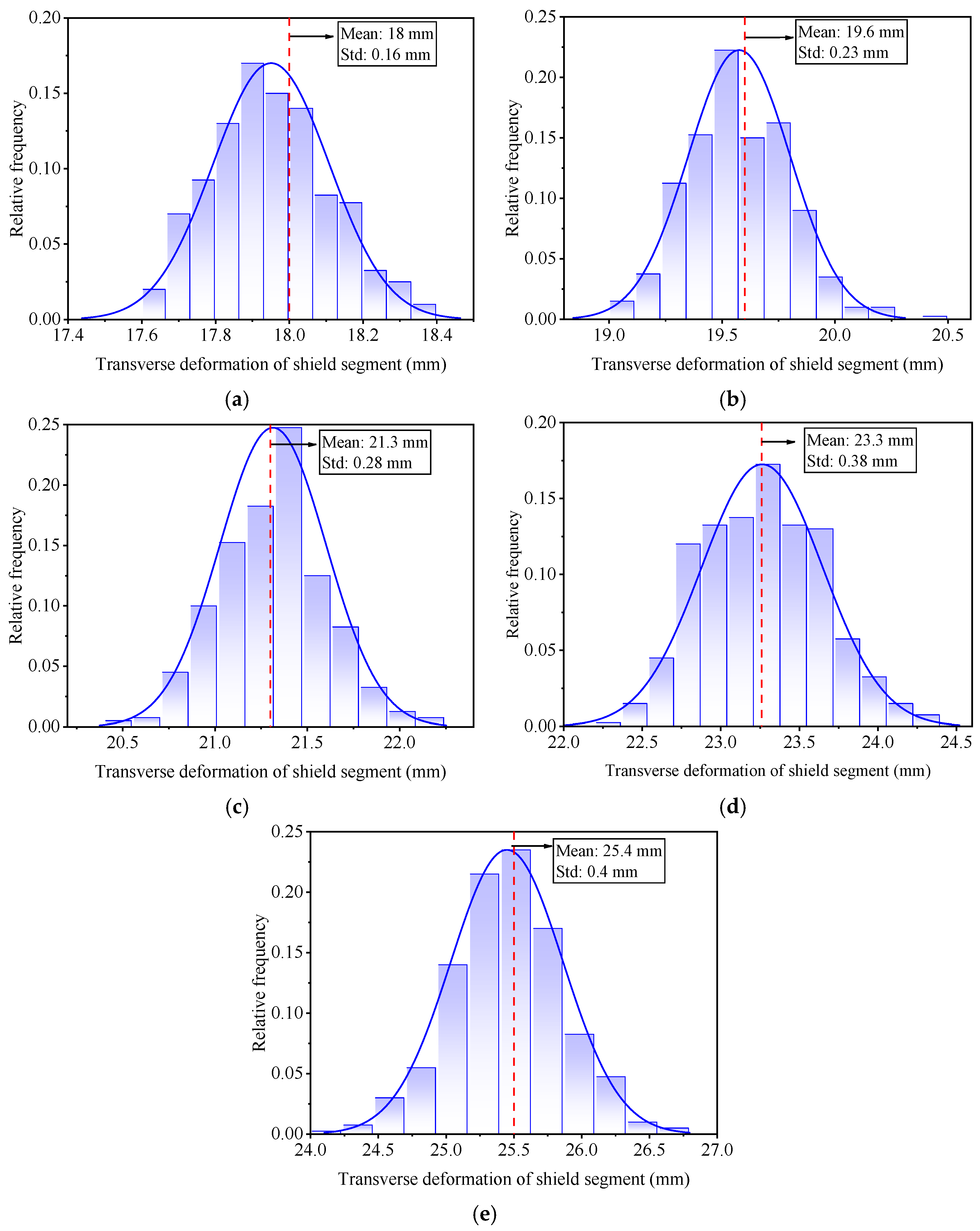
To investigate the effect of the random distribution of structural damage on the transverse deformation of tunnel segments under different damage ratios, a statistical analysis was conducted on all computational results. Figure 8 illustrates the frequency distribution of transverse convergence values for varying damage ratios. It can be observed that, despite the convergence values being predominantly concentrated around the mean, the overall distribution patterns differ across different damage levels.

Firstly, as the damage ratio increases, the overall stiffness of the segment gradually decreases, leading to an increase in both the range and mean value of transverse convergence. Additionally, the standard deviation (Std) also increases, which is attributed to the enhanced nonlinearity of the deformation process at higher damage levels. When the damage ratio increases from 0.1 to 0.5, the mean and Std of the transverse deformation increase by 41% and 150%, respectively. This indicates that deformation becomes more unstable, with a greater occurrence of outliers, thereby posing higher structural safety risks. The results further demonstrate that structural damage exhibits a cumulative effect on segment deformation—higher damage levels lead to greater uncertainty and increased safety risks. Therefore, accurately predicting tunnel deformation under varying damage conditions is crucial for ensuring structural integrity and safety.

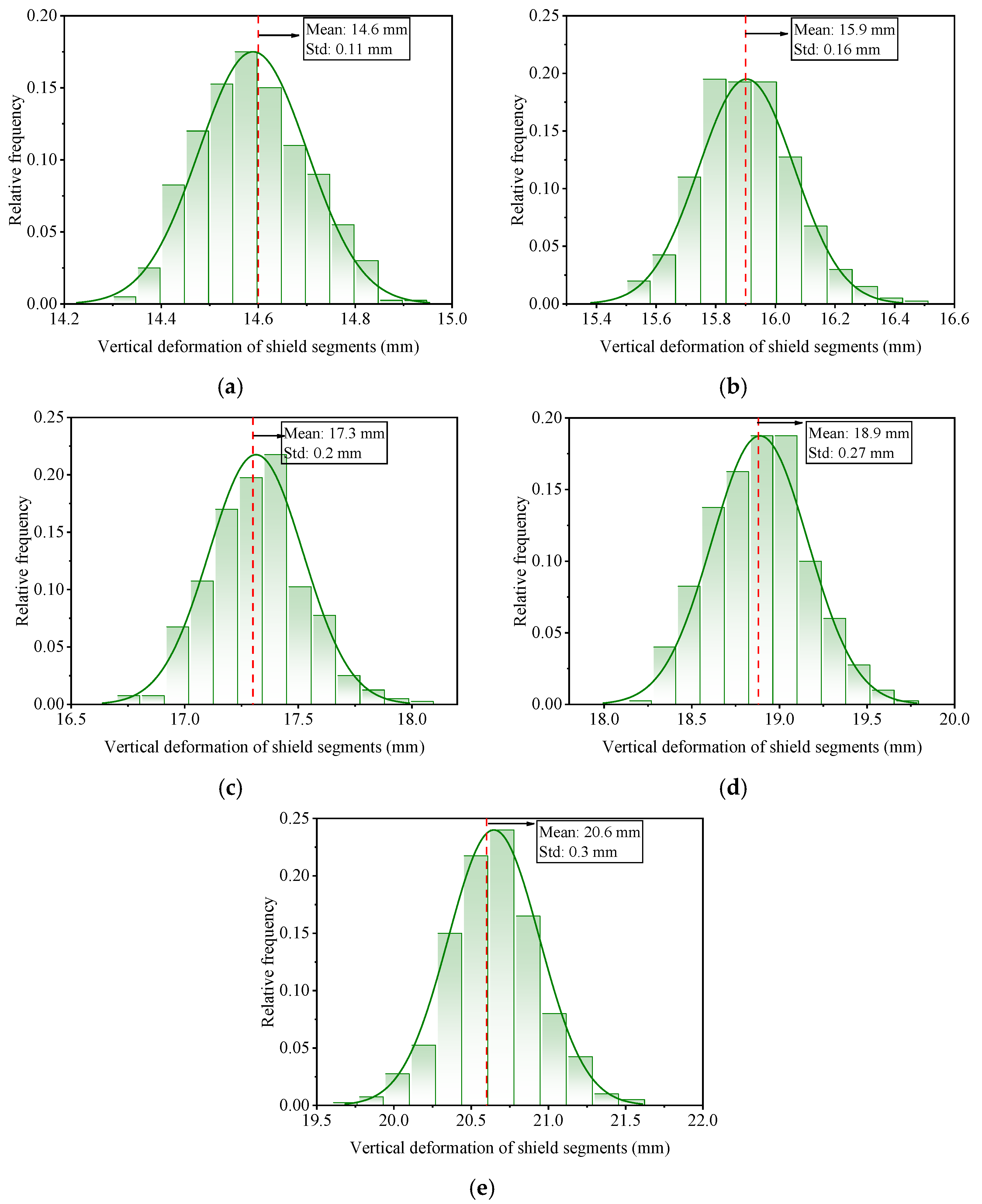
Figure 9 illustrates the frequency distribution of vertical convergence values for varying damage ratios. As observed in Figure 9, both the mean and variability of vertical deformation increase with the damage ratio, following a pattern similar to that of the transverse deformation. However, for the same damage ratio, the mean and range of vertical deformation are consistently smaller than those of transverse deformation, indicating that the vertical convergence of the segment remains lower than its transverse convergence throughout the deformation process. Furthermore, the increasing trend in vertical deformation reinforces the significant impact of damage ratio on deformation uncertainty. As the level of damage intensifies, the probability of large deformation values increases considerably, highlighting the progressive reduction in structural stability.

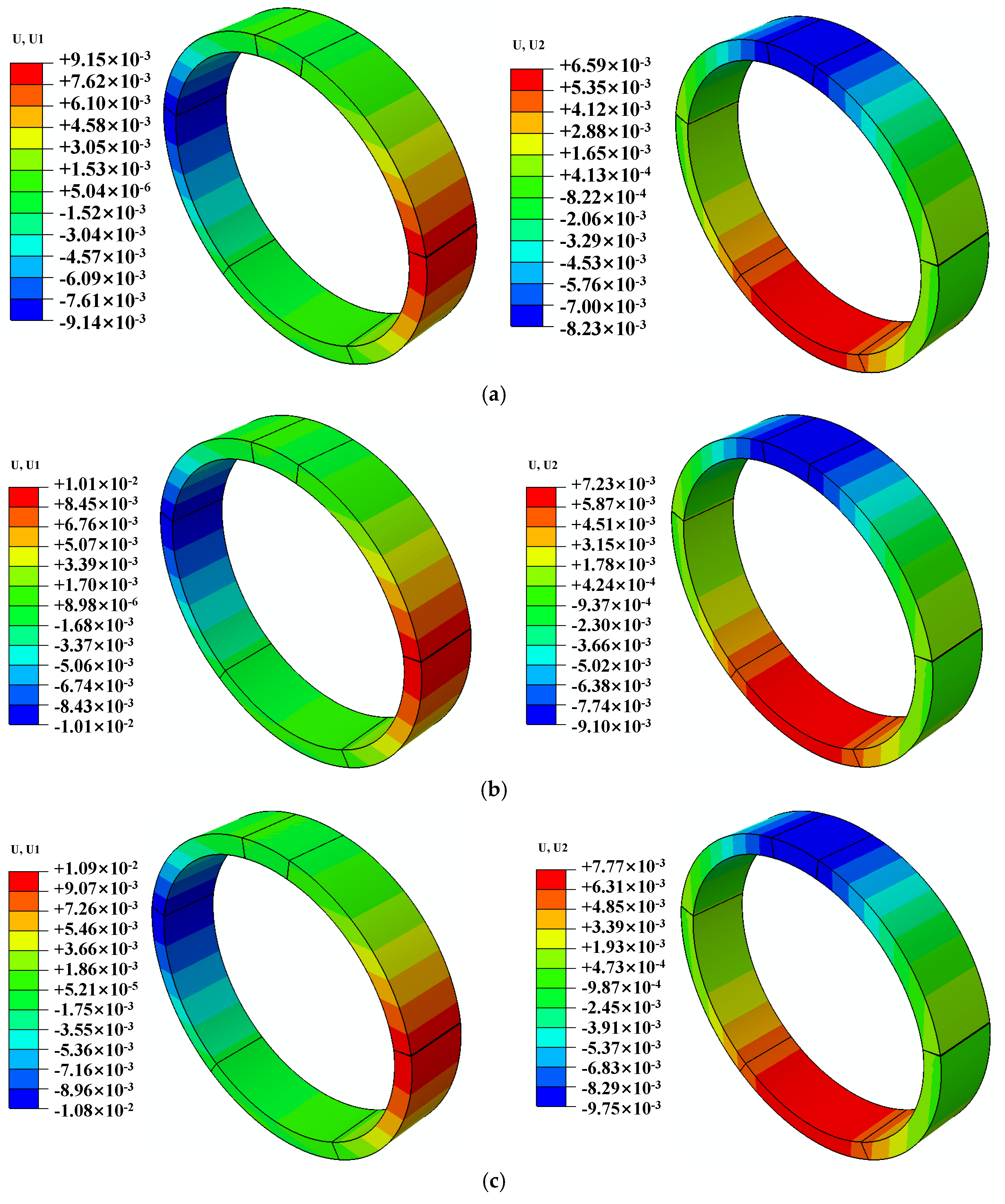
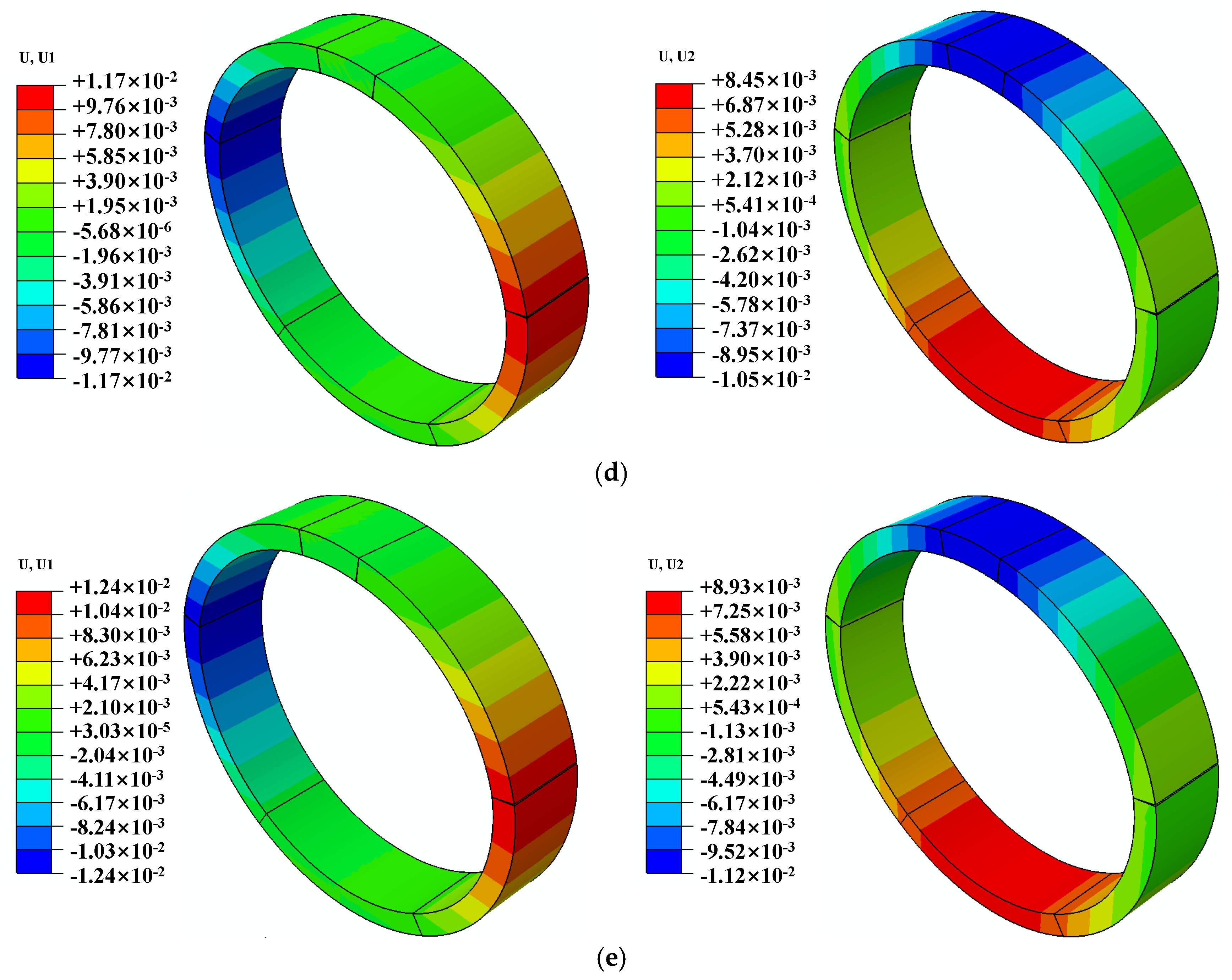
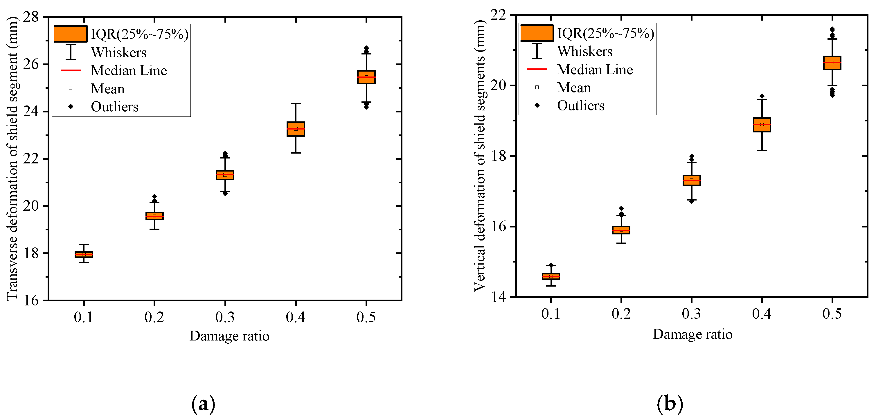
Figure 10 is the typical representative of vertical and transverse deformation nephograms of shield segments under different random damage ratios. Figure 11 presents box diagrams of the calculated deformation results for shield tunnel segments. This can be seen in Figure 10: with an increase in the random damage proportion of shield segments, the vertical and transverse deformation values of shield segments gradually increase, which once again confirms that the random damage proportion will reduce the stiffness of shield segments and increase the deformation. As shown in Figure 11, the mean values of both transverse and vertical deformations increase progressively with the damage ratio, indicating a significant influence of damage severity on segment deformation. The changes in the median and mean values reveal that their differences remain consistently small across different damage ratios, suggesting that the deformation data distribution was relatively symmetrical without noticeable skewness. Furthermore, as the damage ratio increases, the interquartile range (IQR) gradually expands, indicating an increase in deformation dispersion and a widening in the overall data distribution. Simultaneously, the whiskers extend progressively longer, reflecting an expansion in the range of extreme values, with some samples exhibiting significantly larger deformations than the general trend, particularly in the vertical deformation. Additionally, the presence of outliers in groups with higher damage ratios suggests that, under severe damage conditions, abrupt deformations may occur in certain measurement points, highlighting the intensified local deformation effects caused by increased damage severity.

4. Architecture of Proposed 1D-CNN

To develop an efficient surrogate model for tunnel deformation prediction, it is important to select an architecture suited to the spatial nature of the input data. In this study, the input represents the spatial distribution of Young’s modulus across tunnel segments. Convolutional neural networks (CNNs) have been widely applied to similar spatial learning problems and have demonstrated promising performance in related engineering tasks [40,41,42,43]. Compared to multilayer perceptrons (MLPs) and long short-term memory (LSTM) networks, 1D-CNN is more effective at capturing local spatial patterns, which are critical for modeling the influence of localized stiffness degradation. It also offers better generalization and computational efficiency with fewer parameters. Therefore, 1D-CNN was adopted as the core architecture in this work. The convolutional neural network (CNN) is a classical deep learning model originally designed for image processing tasks [44,45,46]. In recent years, CNNs have also demonstrated strong performance in various regression problems. Typically, CNNs consist of multiple layers, with the classic VGG19 network comprising 19 layers [47]. Each layer in a CNN performs a distinct operation to facilitate the extraction of features from the input data. The core components of a CNN include the Convolutional Layer, the Pooling Layer, and the Fully Connected Layer. Figure 12 shows the architecture of the one-dimensional convolutional neural network (1D-CNN) model established in this paper. Below is a brief introduction to the architecture of the 1D-CNN model. The model was trained using the Adam optimizer with an initial learning rate of 0.001. To enhance training stability and mitigate the risks of gradient explosion and vanishing, layer normalization was applied after each convolutional layer. The mean squared error (MSE) was adopted as the loss function. The batch size was set to 64, and the model was trained for 1000 epochs, during which it demonstrated stable convergence. Model parameters were initialized using PyTorch 2.5.1’s default initialization settings. The training was conducted using the PyTorch 2.5.1 framework on a platform equipped with an Intel i7-12700U processor and 32 GB of RAM. To improve generalization performance, a dropout layer with a dropout rate of 0.3 was incorporated into the fully connected layers.

4.1. Convolutional Layer

The convolutional layer (Conv) is the core component of a CNN. The convolution operation involves sliding a set of trainable convolution kernels (or filters) across the input data to extract local features and generate feature maps. In this paper, the Young’s modulus of the concrete in the shield segment under each working condition was used as the input feature. Therefore, the dimensionality of the input feature equals the number of concrete elements, which is 10,816. Each convolution kernel slides over the input data and computes the output at each position of the feature map through weighted summations [48]. This process allows the convolutional layer to effectively identify local patterns in the dataset. This process can be given by Equation (1):

$$y^l=f(w^l*y^{l-1}+b^l)$$

(1)

where, $y^{l-1}$ and $y^l$ denote the input and the output of the $l^{th}$ convolutional layer of the model, $w^l$ an $b^l$ denote the kernel and bias of the $l^{th}$ convolutional layer of the model, $f(\cdot )$ denotes the activation function, and the symbol “*” denotes the convolution operation. The training task of the convolutional layer is to learn a set of optimal convolution kernels through backpropagation, which can then be used for feature extraction and prediction. In this paper, two convolutional layers are used, with output channels of 64 and 32, respectively. The key hyperparameters of the convolutional layer include kernel size, stride, and padding. In this study, these parameters were set to 3, 1, and 1, respectively.

4.2. Pooling Layer

The pooling layer (Pool) is typically placed after the convolutional layer, and its primary function is to reduce the size of the data while preserving the most significant feature information [49]. The pooling operation decreases the computational complexity by processing local regions of the input feature map, while retaining key features. Common pooling operations include max pooling and average pooling: max pooling selects the maximum value from each local region as the representative of that region, while average pooling computes the average value of the local region. Equation (2) presents the computation process of the average pooling layer:

$$p^l={\displaystyle \frac{1}{m}}{\displaystyle \sum a_{win}^l}$$

(2)

where $p^l$ denotes the output feature map of the lth pooling layer, m is the pooling window size, and $a_{win}^l$ denotes the values within each pooling window of the lth layer. The pooling layer serves to reduce the size of the feature map and alleviate the computational burden of subsequent layers. In this paper, the average pooling layer with a size and stride size of 3 was selected.

4.3. Fully Connected Layer

The fully connected layer (FC) is located at the final stage of the neural network and is typically responsible for performing the final classification or regression task. In this layer, each neuron is connected to all the neurons in the previous layer. Its primary function is to integrate the local features extracted through the convolutional and pooling layers and make the final decision. The fully connected layer combines the outputs of each neuron using weighted summations and activation functions, ultimately producing the final classification or regression prediction. The calculation of the fully connected layer is shown in Equation (3):

$$z^l=f(W^{l-1}{p}^{l-1}+b^{l-1})$$

(3)

where $p^{l-1}$ denotes the input to the (l−1)^th fully connected layer, either from the final pooling layer (flattened) or the preceding fully connected layer, $W^{l-1}$ and $b^{l-1}$ represent the weight matrix and bias term of the (l−1)^th fully connected layer, and $z^l$ represents the activated output passed to the lth fully connected layer. In this paper, three fully connected layers were used, and the number of neurons in each layer was 256,128 and 64, respectively. At the end of the convolutional neural network, the transverse deformation and vertical deformation of the segments in each working condition are taken as the prediction results, so the output size of the model is 1 × 2.

4.4. Activation Function

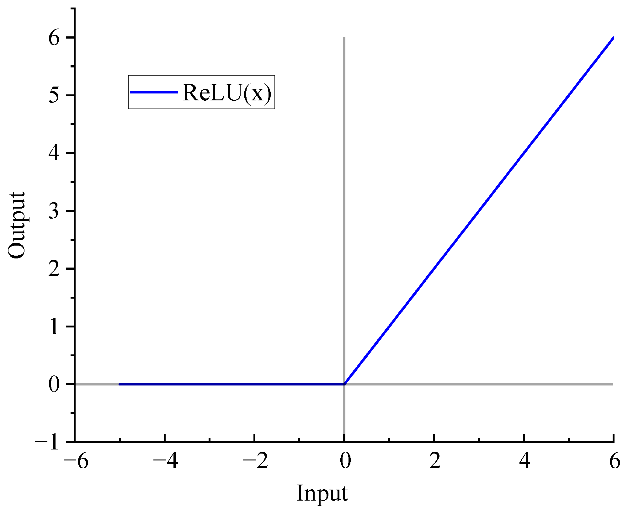
The Rectified Linear Unit (ReLU) is a widely used activation function in deep learning [31], particularly in convolutional neural networks (CNNs) and feedforward neural networks (FNNs). Its mathematical expression is given by ReLU(x) = max(x, 0). Incorporating ReLU into neural networks enables the model to learn nonlinear relationships, allowing it to capture more complex features. Compared to traditional activation functions such as sigmoid and tanh, ReLU is computationally more efficient as it only requires a simple maximum operation. As shown in Figure 13, in the positive domain (x > 0), ReLU maintains a constant gradient of 1, preventing the gradient vanishing issue commonly observed in sigmoid and tanh functions, which facilitates deep network training. In the negative domain (x ≤ 0), ReLU outputs zero, effectively deactivating certain neurons, which enhances network sparsity and improves generalization performance. Considering its advantages in computational efficiency, gradient stability, and model generalization, this study adopts ReLU as the activation function in the proposed neural network model.

5. Surrogate Model Performance

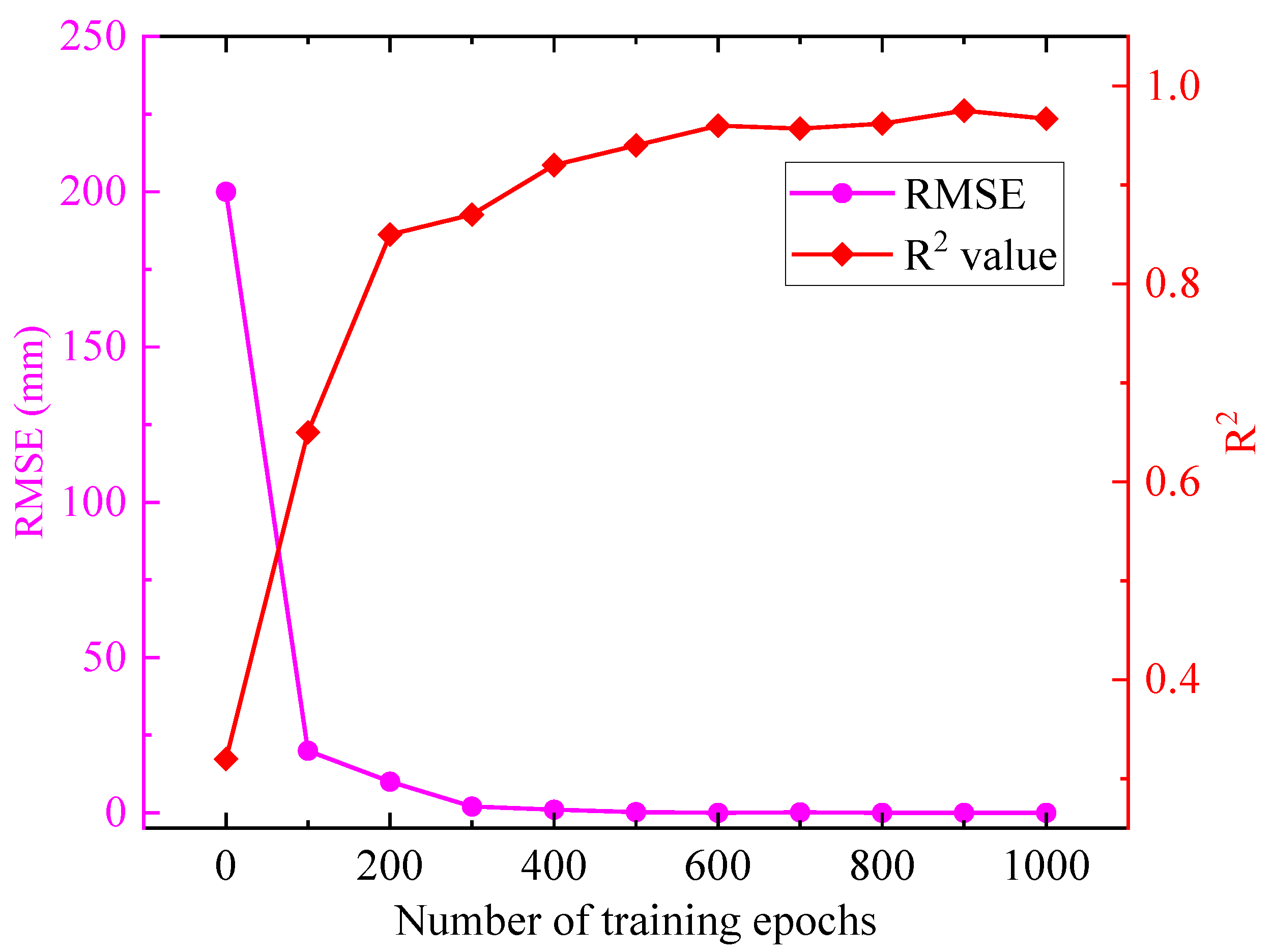
As mentioned above, 400 sets of random finite element analyses were conducted for each damage ratio, resulting in a total of 2000 samples for deep learning. For each damage ratio, 20% of the samples were reserved as the test set, while the remaining samples were collectively used to form the training set. Figure 14 illustrates the variation of the root mean square error (RMSE) and the coefficient of determination (R²) with increasing training epochs for a damage ratio of 0.5 in shield tunnel segment transverse displacement prediction. As shown in Figure 14, the RMSE decreases rapidly with more training epochs and eventually stabilizes, indicating that the model error converges and the prediction accuracy improves significantly. Meanwhile, the R² value exhibits an upward trend, ultimately approaching 1.0, demonstrating an enhanced model fitting capability. When the number of training epochs reached 1000, both the RMSE and R² converged, suggesting that the model had nearly reached its optimal state. Therefore, the 1D-CNN surrogate model proposed in this study can perform well after 1000 epochs of training.

5.1. Model Performance on Transverse Deformation

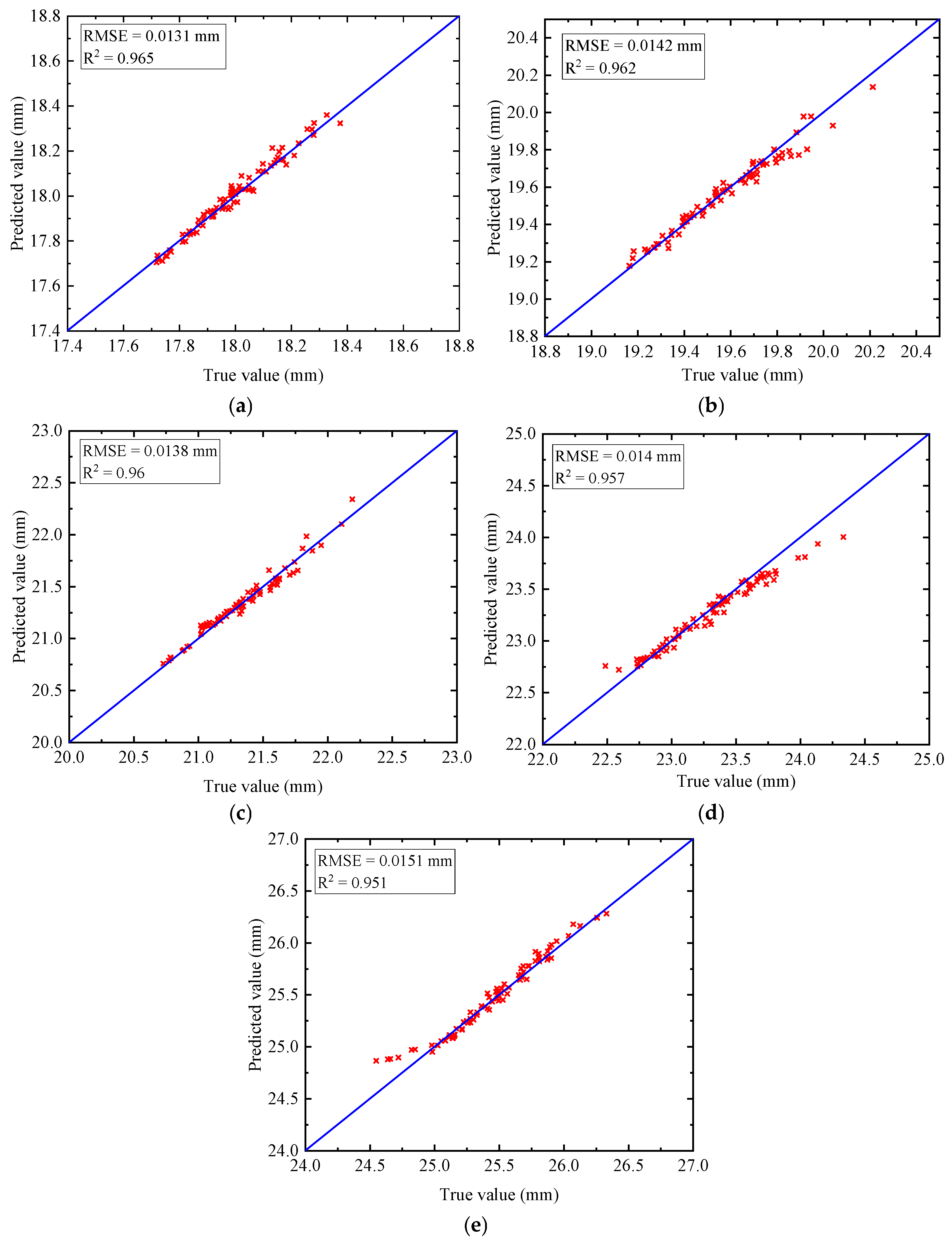
Figure 15 presents the prediction results of the 1D-CNN model on the test set for the transverse displacement of shield tunnel segments, with FEM calculations serving as the true value. In Figure 15, each red “x” represents a data point where the horizontal axis corresponds to the true value and the vertical axis corresponds to the predicted value. When the scatter points align along the diagonal line (y = x), it indicates that the model’s predictions closely match the true values, demonstrating good predictive performance. To further quantify the model’s accuracy, the root mean squared error (RMSE) and correlation coefficient R² are employed as evaluation metrics. A smaller RMSE and aR² value closer to 1 indicate a superior predictive performance. From the scatter plots at different damage ratios, it is evident that the 1D-CNN model maintains a high level of agreement with the FEM results, with R² values exceeding 0.95 and RMSE values remaining below 0.016 mm across all conditions, confirming the model’s high accuracy. Additionally, at lower damage ratios, the data points are more concentrated, indicating minimal error. As the damage ratio increases, the predictions remain generally accurate; however, the dispersion of data points slightly increases, and some points deviate from the diagonal, suggesting that prediction errors tend to rise under high-damage conditions. Overall, the 1D-CNN model effectively captures the variation patterns of transverse displacement in shield tunnel segments across different damage ratios, demonstrating a stable predictive performance, high reliability, and strong generalization ability.

5.2. Model Performance on Vertical Deformation

Figure 16 presents the prediction results of the 1D-CNN model on the test set for the transverse displacement of shield tunnel segments. The red “x” markers have the same meaning as in Figure 15. The prediction results for vertical displacement indicate that the 1D-CNN model maintains consistently high accuracy across different damage ratios. The scatter points are closely distributed along the diagonal line (y = x), demonstrating a strong agreement between the predicted and actual values. Across all conditions, R² for vertical displacement exceeds 0.95, while the RMSE remains below 0.014 mm, further validating the model’s reliability. Compared to transverse displacement, the prediction results for vertical displacement exhibit a more concentrated distribution, suggesting that the model performs more stably in predicting vertical deformation. This may be attributed to the relatively smooth variation in vertical displacement, allowing the model to capture its patterns more accurately. However, at higher damage ratios, the prediction error tends to increase slightly, which may be due to the growing complexity and nonlinearity of damage progression.

5.3. Model Prediction Error

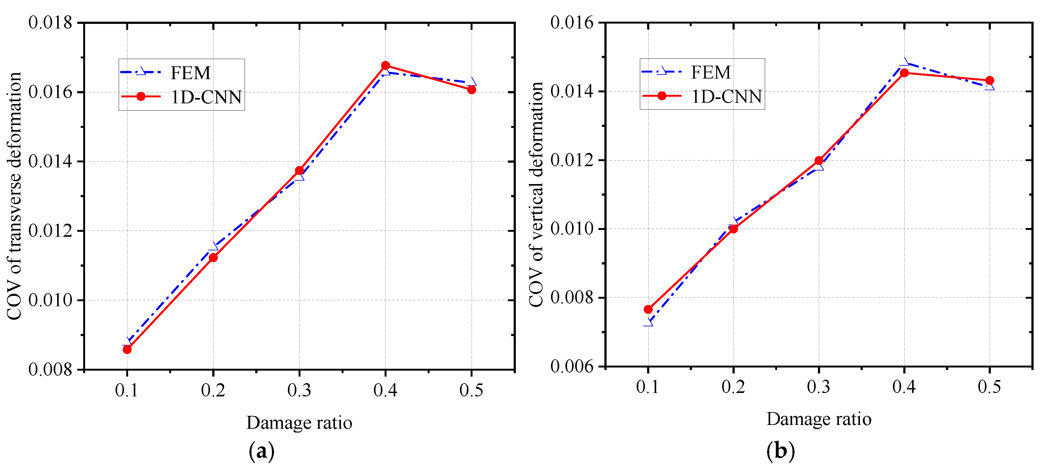
To further investigate the statistical characteristics of the prediction results, a comparison between the COV values of segment deformation predicted by 1D-CNN and those calculated by FEM was conducted in the testing set, as shown in Figure 17. From Figure 17a,b, it can be observed that the developed model accurately predicts the variation trend of the COV values of segment deformation under different damage ratios. Specifically, as the damage ratio increases, the COV of segment deformation gradually rises. The comparison results indicate a high level of consistency between the COV values predicted by 1D-CNN and those computed by FEM, demonstrating that 1D-CNN effectively captures the statistical distribution characteristics of FEM results. This finding confirms the feasibility and reliability of 1D-CNN in such prediction tasks.

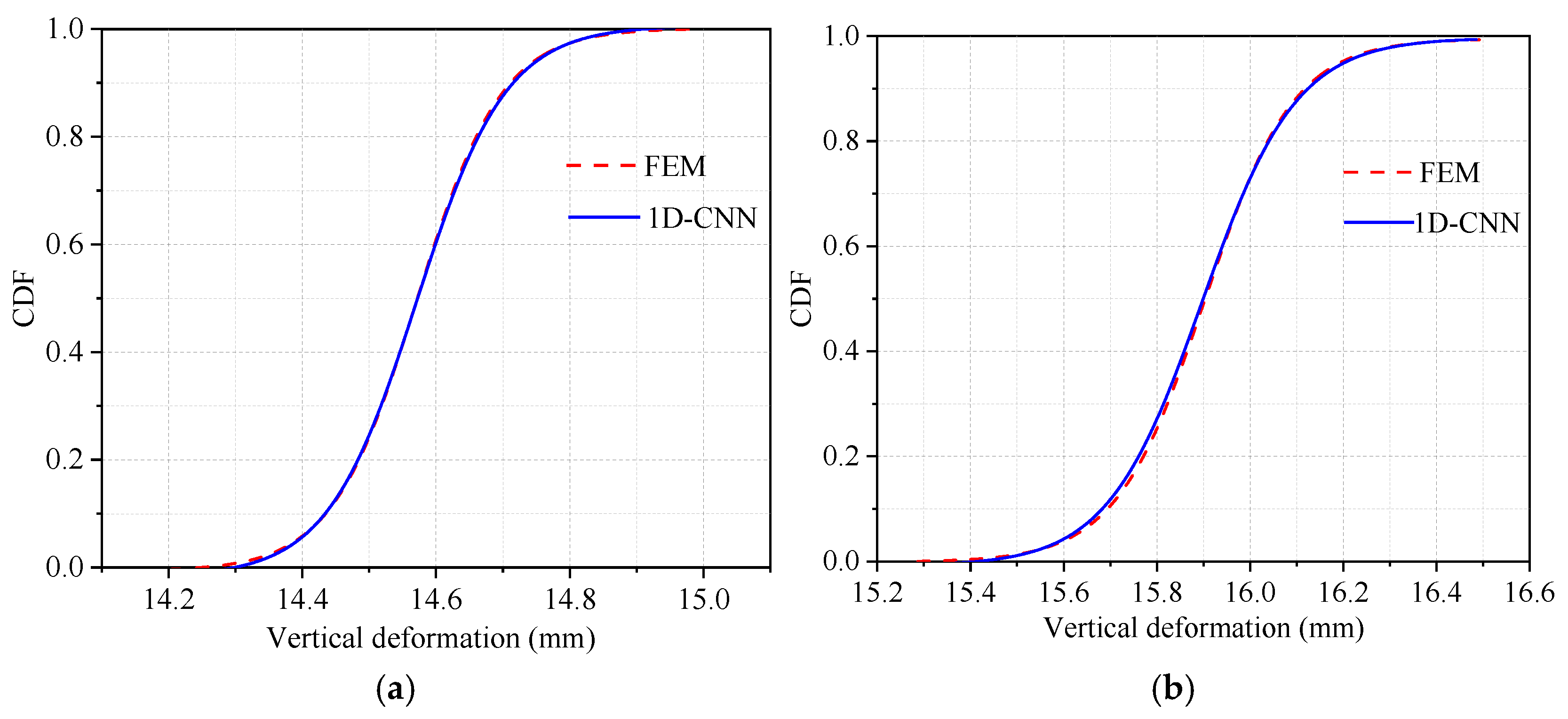
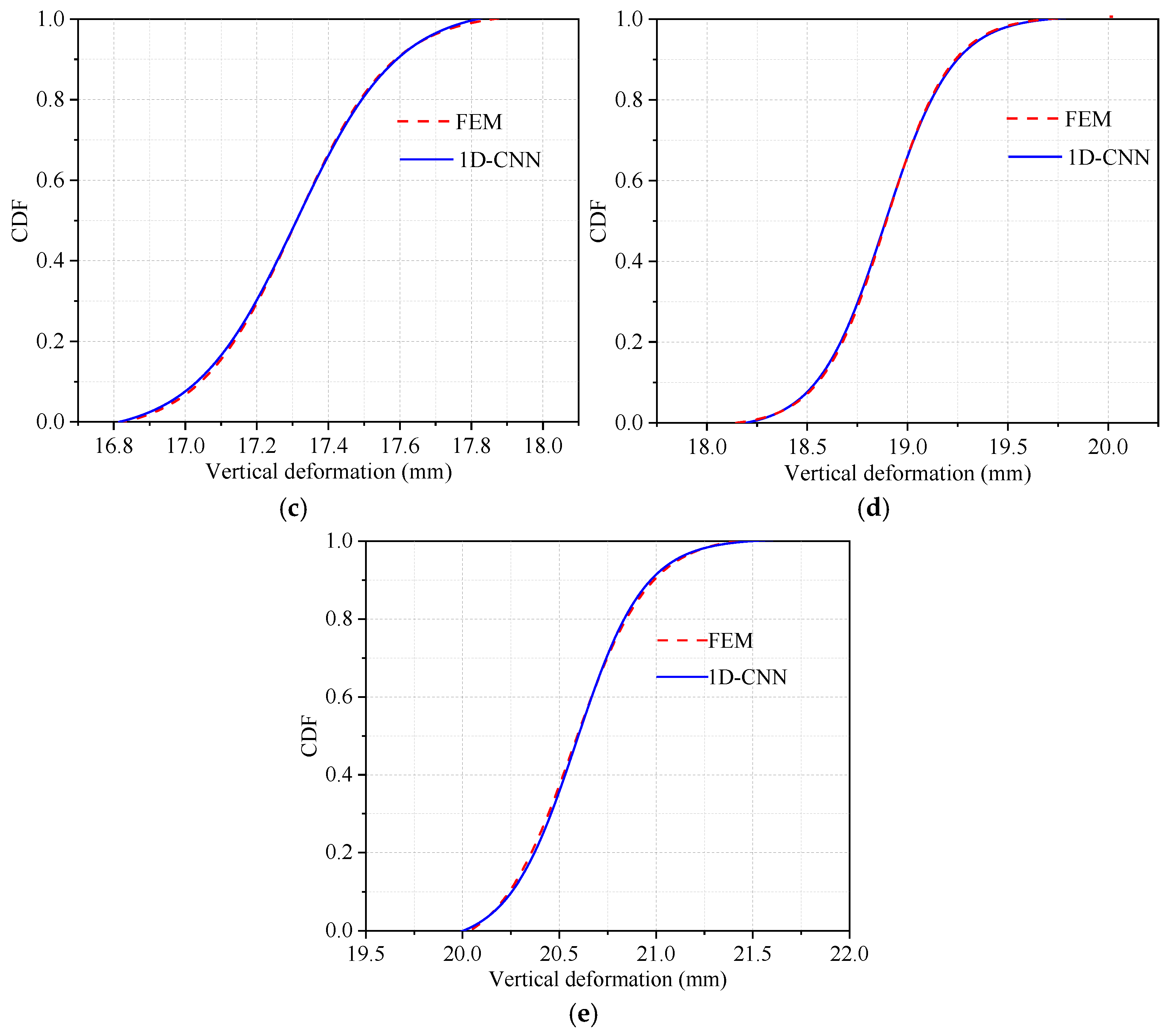
Figure 18 and Figure 19 respectively compare the cumulative distribution functions (CDF) of transverse and vertical deformations of the shield tunnel, as obtained from finite element simulations and predicted by the 1D convolutional neural network (1D-CNN), across test sets with varying damage ratios. The substantial overlap between the two curves indicates a high level of agreement in the overall statistical distribution of shield segment deformation, thereby validating the predictive capability of the proposed 1D-CNN model. Furthermore, to quantitatively assess the accuracy of 1D-CNN predictions,

Table 1. Relative error of the statistics of transverse deformation of segments.

Damage Ratio	0.1	0.2	0.3	0.4	0.5
Min	2.12%	0.96%	1.71%	3.01%	1.54%
Mean	0.23%	0.19%	0.32%	0.20%	0.11%
Max	3.10%	2.03%	3.21%	2.32%	3.31%

and

Table 2. Relative error of the statistics of vertical deformation of segments.

Damage Ratio	0.1	0.2	0.3	0.4	0.5
Min	1.55%	3.41%	0.98%	2.11%	1.17%
Mean	0.55%	0.24%	0.63%	0.27%	0.15%
Max	1.21%	2.04%	2.54%	1.98%	2.88%

present the relative errors of various statistical metrics between the FEM calculations and 1D-CNN predictions for the transverse and vertical deformations of the shield segment deformation. As observed in Table 1 and Table 2, the relative errors of the statistical metrics for both transverse and vertical deformations remain consistently low across different damage ratios. For transverse deformation, the maximum relative errors for the minimum value (Min), mean, and maximum values (Max) are 3.01%, 0.32%, and 3.31%, respectively. Similarly, for vertical deformation, these values are 3.41%, 0.63%, and 2.88%. The consistently low relative errors further validate the strong predictive performance of the 1D-CNN model, indicating that the statistical distribution of 1D-CNN predictions closely aligns with the FEM results. This highlights the reliability of 1D-CNN for engineering prediction tasks of this nature. These consistently low relative errors demonstrate that the 1D-CNN model reliably captures both the central tendency and extreme values in tunnel deformation prediction.

5.4. Limitations and Application

The finite element model and 1D-CNN surrogate model developed in this study demonstrated satisfactory performance in predicting the deformation behavior of shield tunnel segments. However, several limitations remain that warrant further improvement. Due to the high computational cost of three-dimensional finite element simulations, the size of the training dataset is inherently limited, which constrains the model’s learning and generalization capabilities—particularly under severe damage conditions. The FEM approach simulates random damage by reducing the Young’s modulus of concrete elements, effectively representing stiffness degradation but failing to capture more complex mechanisms such as segment cracking or reinforcement corrosion. While the 1D-CNN model achieves high overall accuracy, prediction errors tend to increase at higher damage ratios, likely due to increased uncertainty and variability in structural response as stiffness deteriorates.

To further enhance the robustness and generalization capability of the proposed framework, future work may consider incorporating more advanced damage models, including those that account for progressive cracking, material deterioration, and various tunnel cross-sectional geometries. Additionally, data augmentation strategies may be employed to enrich the training dataset, particularly under high-damage scenarios.

Beyond its technical contributions, the proposed approach also shows promise for practical implementation in tunnel condition assessment. With the rapid advancement of tunnel monitoring technologies, a solid foundation has been established for integrating numerical simulation with field-observed structural behavior.

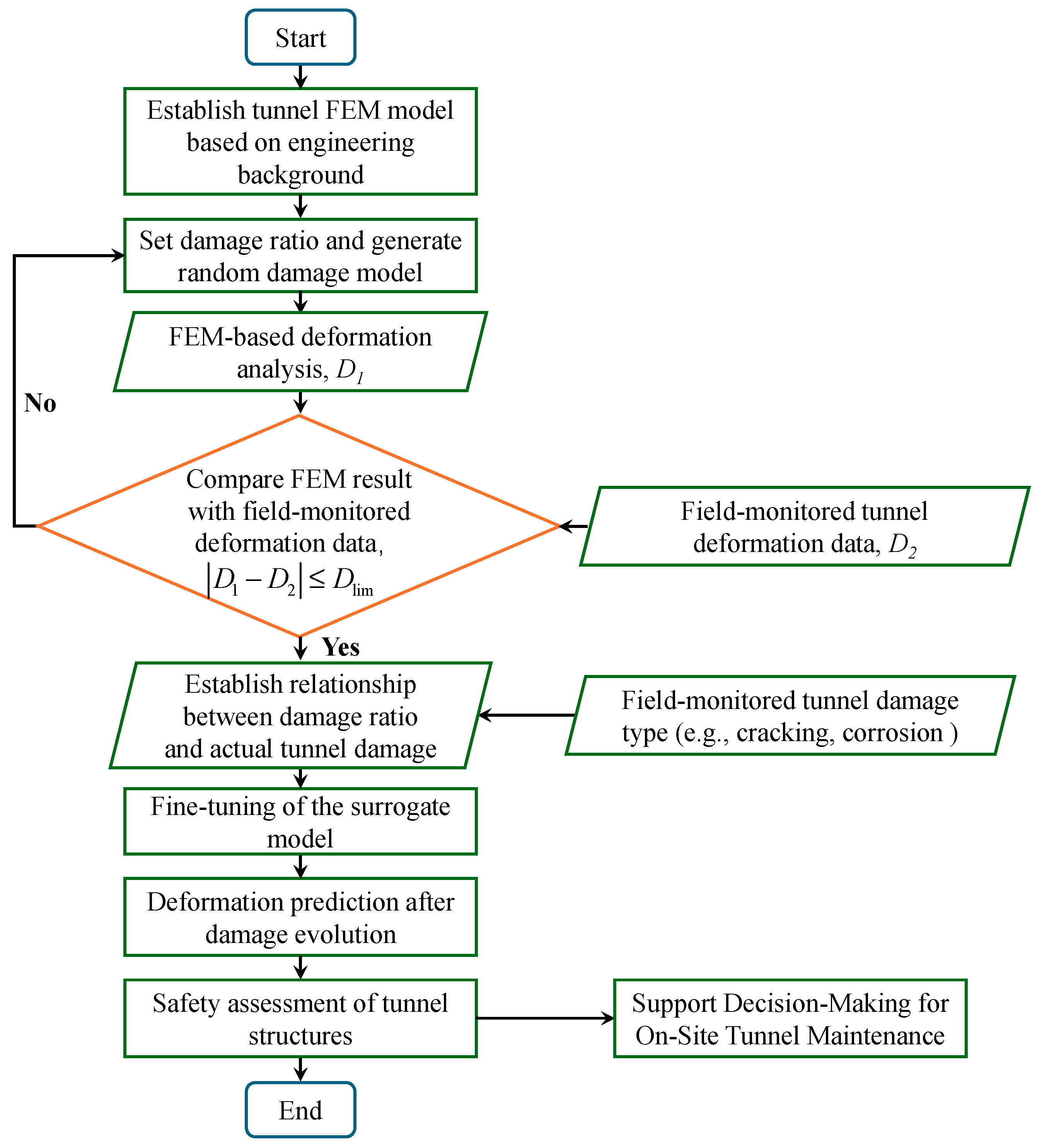
As illustrated in Figure 20, an application-oriented workflow is proposed to integrate field-monitored deformation data with the FEM–surrogate modeling approach developed in this study. In this framework, a tunnel finite element model is first established based on the engineering background to reflect the actual structural characteristics. Then, deformation results from a random-damage FEM model (D₁) are compared with field-monitored deformation data (D₂). When the difference between the two falls within a predefined threshold (D_lim), the FEM model can be considered to approximate the actual tunnel state with reasonable accuracy. This comparison provides a potential basis for linking simulated damage ratios with real-world tunnel damage types (e.g., cracking, spalling), thereby connecting numerical modeling with physical deterioration. Based on this correlation, the surrogate model may be fine-tuned using field-identified damage data to improve its applicability under practical conditions. Once calibrated, the model is expected to efficiently predict tunnel deformation under varying damage evolution scenarios. Finally, the safety status of the tunnel structure can be evaluated in accordance with relevant technical standards, providing a reliable basis for maintenance decision making.

Taken together, this study outlines a promising framework that bridges numerical simulation, machine learning, and field monitoring, contributing to both the theoretical understanding and practical management of shield tunnel performance.

6. Conclusions

This study successfully developed a finite element modeling (FEM) framework for simulating random damage in shield tunnels and analyzed the impact of varying random damage proportions on segment deformation. Additionally, a 1D-CNN surrogate model was constructed and trained using FEM simulation results to mitigate the high computational cost associated with FEM analysis. The performance of the proposed surrogate model was comprehensively evaluated. The key findings of this study are as follows:

(1) A random damage simulation framework was proposed, enabling the simulation of random damage in shield tunnel segments. The computational results indicate that as the damage ratio increases, both the range and mean values of segment deformation increase, leading to greater instability and a higher structural safety risk.

(2) The proposed 1D-CNN model effectively predicts shield tunnel deformation under different damage ratios. The root mean square error (RMSE) for all training datasets is below 0.016 mm, and the coefficient of determination (R²) exceeds 0.95. The prediction results suggest that this model provides a novel approach for analyzing damage-induced deformation in shield tunnels.

(3) The statistical differences between the 1D-CNN model predictions and FEM simulation results are minimal, demonstrating that the model can accurately capture the statistical distribution of shield segment deformation under varying random damage conditions. This underscores the effectiveness and reliability of the proposed surrogate model.

(4) A practical framework is proposed to integrate FEM-based damage simulation with monitoring data, thereby enhancing the applicability of the 1D-CNN surrogate model for tunnel deformation prediction and supporting safety evaluation and maintenance planning.