Fatigue Life of Pre-Cut Seam Asphalt Mixture Composite Beams: A Combined Study of Fatigue Damage Evolution and Reflective Cracking Extension

Abstract

This study investigated the impact of reflective cracking on the fatigue performance of asphalt pavements after milling and resurfacing under various conditions. Fatigue life was assessed through four-point flexural fatigue tests, while the crack extension pattern of composite beams was analyzed by digital image correlation (DIC) at both macroscopic and microscopic scales. Evaluation parameters such as stress ratios, immersion time, porosity, and types of viscous oils were assessed. A fatigue life prediction model of composite beams was established, accounting for the combined influence of these factors. To enhance the accuracy of determining composite beam failure, the critical fatigue damage was calculated by defining the damage variable in terms of the dynamic modulus. A nonlinear fatigue damage model was proposed, incorporating this critical damage under the combined influence of various factors. Additionally, a modified logistic function model was developed to describe the relationship between crack extension and failure life under different stress ratios, porosities, and viscous layer oil conditions. It was found that the modulus decay curves and the crack extension curves intersected at different stress levels as the life ratio increased. At the intersection, the modulus ratios were consistently around 0.55, marking the transition of the specimen from a stable to an unstable state. Beyond this point, the crack rapidly propagated, leading to a sharp reduction in the modulus until the specimen ultimately failed. Our results provide a basis for timing and conservation decisions.

1. Introduction

The predominant structural configuration of asphalt pavement in China is semi-rigid base asphalt pavement, which is prone to reflective cracking. These cracks typically propagate from the subgrade up to the asphalt surface. However, milling and resurfacing can only treat about 4 cm of the surface layer. If reflective cracks in the original pavement are not properly treated beforehand, they can easily penetrate through this thin overlay. While pretreating reflective cracks can help, it significantly increases the workload and slows down construction progress [1,2,3]. Additionally, there are high rates of interlayer debonding, dynamic water damage, and porosity [4,5,6]. The appearance of cracks will make it very easy for surface water to infiltrate into the structure. The gap water will migrate freely along the gap under the joint action of the natural environment and vehicle loading and produce localized damage, thus exacerbating the impact of cracks in the resurfacing cover, the process of its impact is shown in Figure 1.

Asphalt mixtures, as viscoelastic materials, exhibit mechanical behavior that is significantly influenced by factors such as temperature, load, and moisture. Most researchers have investigated the fatigue mechanical behavior of single-layer asphalt mixtures [7,8,9]. However, the pavement structure is composed of a multi-layer asphalt mixture. Therefore, the study of composite beam structural layers provides a more accurate representation of real-world pavement conditions. In China, research on composite beam structure has primarily focused on two-layer systems involving water-stabilized and asphalt layers, whereas studies on dual-layer asphalt mixture composite beams are relatively limited [10,11]. Milling and resurfacing overlay refers to milling off the damaged surface layer of asphalt pavement to resurface it with a new asphalt layer to improve the life of asphalt pavement [12]. Jin et al. added tire rubber (GTR) to a resurfaced asphalt pavement. The results showed that GTR gives asphalt pavements better cracking resistance while also reducing noise [13,14]. Currently, research on the milling and resurfacing of asphalt pavements mainly focuses on construction technology, milling material, and material recycling [15,16,17,18]. There are few studies on the effect of reflection cracks on the damage pattern and fatigue life of asphalt pavements after milling and resurfacing under multiple factors. In this paper, the effects of reflective cracking on milled and resurfaced asphalt pavements are considered based on stress level, immersion time, void ratio, and viscous oil. The damage law is clarified, and a fatigue life prediction model is proposed, deepening the theory and methodology of milling and resurfacing asphalt pavement design. Chinese scholars have begun to address this gap, focusing on the actual stress conditions of composite pavements and the fatigue behavior of multi-layer asphalt mixtures. Liao et al. investigated the mechanical interlayer properties of dual-layer porous asphalt samples using a variety of compaction methods. They found that samples compacted by hot-heat compaction had higher shear and ultimate tensile strengths, which were inversely related to the fractal dimension [19]. Yang et al. proposed an interlayer stability evaluation method. The analysis is based on the principle of shear fatigue, modeling, and the axial load conversion method after using direct shear fatigue test studies on asphalt mixture composite beams with five different binder layers [20].

In this study, digital image correlation technology is employed to monitor crack development in composite beam experiments. DIC is a non-contact deformation testing technique built on the principles of computer vision and digital image processing. It offers several advantages, such as non-contact, whole-field measurement, simple instrumentation, and powerful anti-jamming capability [21]. In recent years, the DIC technique has been adopted to study the fracture behavior of asphalt mixes [19,22], which has proved the feasibility and superiority of digital scatter correlation methods in civil engineering [23,24,25,26]. Since the introduction of DIC into the civil engineering field, various parameters have been investigated to evaluate the quality of the scattering sample, including root mean square error [27], scatter size [28], scatter coverage [29], average gradient [30], and the square of the gradient of the intensity of the subset [31]. In recent years, the DIC technique has mainly been used to study the crack extension law of concrete. Li et al. used a three-point bending test on concrete composite beam specimens while using the DIC technique to observe the crack extension law. Thus, they proposed a method to determine the location of the tip of concrete cracks and the fracture process zone (FPZ) [32]. However, there are fewer studies on asphalt mixtures using this technique. It is, therefore, necessary to observe surface crack extension patterns of precast seamed asphalt composite beams under flexural fatigue using the DIC technique. The organizational flowchart of this paper is shown in Figure 2.

The main objective of this paper is to investigate the effect of reflection cracks on the fatigue performance of asphalt pavements after milling and resurfacing under different influencing factors. The specific work is as follows: (1) In this study, the fatigue mechanical behavior of pre-cut cracked asphalt mixtures was evaluated using a four-point bending fatigue test under stress control, taking into account the effects of stress level, type of viscous layer oil, water immersion time, and void ratio. (2) A fatigue life prediction model for asphalt mixture composite beams under the combined influence of different factors is presented. (3) By defining the dynamic modulus as a damage variable under multiple factors, a nonlinear fatigue damage model for the critical fatigue behavior of composite beams is developed. (4) The DIC correlation technique is used to observe the crack extension. This will help to explore the process of pavement fatigue damage to composite structural layers and understand the fatigue damage behavior of pavement composite layers.

2. Materials and Methods

2.1. Materials

In this study, the overlay utilizes an AC-13C asphalt mixture (optimum asphalt content of 4.8%). The leveling layer employs an AC-20 asphalt mixture (optimum asphalt content of 4.6%). Figure 3 and Figure 4 illustrate the gradation curve for both mixtures. The chosen asphalt materials include 70# A-grade matrix asphalt and SBS-modified asphalt, with their technical specifications detailed in

Table 1. Technical indexes of 70 # asphalt and SBS-modified asphalt.

Pilot Project		70 # Asphalt		SBS-Modified Asphalt
		Result	Requirement	Result	Requirement
Needle penetration (25 °C, 100 g, 5 s) (0.1 mm)		68	60–80	49	40–60
PI		−1.1	−1.5~+1.0	0.237	≥0
Ductility (15 °C, 5 cm/min) (cm)		>100	≥100	-	-
Ductility (5 °C, 5 cm/min) (cm)		-	-	36	≥20
Softening point (°C)		48	≥46	86.0	≥60
60 °C dynamic viscosity (Pa·s)		202.7	≥180	2.3	≤3
Density (15 °C) (g/cm3)		1.032	actual	1.039	actual
Flashpoint (°C)		295	≥260	301	≥230
Solubility (%)		99.8	≥99.5	99.9	≥99
Adhesion with coarse aggregate		5	≥5	5	≥5
Elastic recovery (25 °C) (%)		-	-	78	≥75
48 h softening point difference (°C)		-	-	1.3	≤2.5
After TFOT (or RTFOT)	Mass variation (%)	−0.262	≤±0.6	0.1	≤±1.0
	Residual penetration ratio (25 °C) (%)	66.2	≥61	78	≥65
	Residual ductility (10 °C) (cm)	8	≥6	22	≥15

[33]. Phyllite is utilized as the aggregate for the overlay, while limestone aggregate is selected for the leveling layer.

2.2. Preparation of Specimen

The AC-20 leveling layer is prepared and allowed to rest for 12 h. Then, the AC-13 top layer is applied, ensuring that an adhesive layer of oil (SBS-modified asphalt or 70# matrix asphalt) is uniformly applied between the two layers at a rate of 0.65 kg/m². After milling and molding the asphalt mixture into rutted slabs, the slabs are cut and smoothed to produce composite beam specimens of 37.5 cm, 6.5 cm, and 10 cm in length, width, and height, respectively. Current research on road maintenance using milling and resurfacing technology typically focuses on top-layer milling resurfacing, leaving the middle layer while retaining the original surface [34,35]. To simulate cracks in the original road surface layer, prefabricated joints are introduced at the bottom of the specimen to simulate cracks in the original road surface layer. These joints are 3 ± 0.5 mm wide and 10 ± 1 mm deep.

2.3. Four-Point Bending Fatigue Test

The four-point bending fatigue test for the composite beam is conducted in a stress-controlled mode, with the bending modulus of strength at the 100th cycle taken as the initial value. Currently, there is no established specification for the fatigue test under stress control to define the damage criterion. The most commonly used parameters for estimating fatigue damage in stress-controlled fatigue tests are modulus, strength, etc. Complete specimen failure is considered the damage criterion. However, following the approach of some scholars, the specimen is considered damaged when its modulus decreased to 10% of its initial value. This criterion is adopted in the experiment. Prior to testing, both the specimen and the fixture are placed in an environmental chamber at 20 °C for four hours. The test process is shown in Figure 4. The effects of five stress levels, three immersion times, three viscous layer oils, and three porosities on the fatigue life of combined beams are investigated using the full method.

Table 2. Factors in the four-point bending test and the level of each of the factors.

Factor	Number of Factors	Factor Level Value
Stress level (MPa)	4	0.5, 0.65, 0.8, 0.95
Immersion time (h)	3	0, 48, 120
Viscous layer oil types	3	Non-sticky layer oil, 70#, SBS
Percentage of void (%)	3	2, 4.5, 6,

shows the factors influencing the four-point bending test and their level values. A sinusoidal loading pattern with a frequency of 10 Hz is selected for the test, and each group is tested three times in parallel to ensure accuracy.

2.4. DIC Test

The DIC acquisition system is activated with a Material Testing System (MTS) for simultaneous operation. In this study, white matte paint is first sprayed horizontally or diagonally upwards and allowed to drift down on the surface of the specimen in the area to be tested. Once the paint dries, the surface is pressed to disperse the speckles for optimal DIC tracking. Calibration images are acquired using Digital Image Correlation System (VIC-3D) snap software. After the DIC test, the crack extension of the specimen is analyzed by VIC-3D 9 software. Since the test has been designed for type I fractures, the crack extension path shows minimal deflection. Therefore, the test area is set at the center of the specimen, with the size of 60 mm × 100 mm, to ensure that the DIC method observes the complete crack extension process. The acquisition process is shown in Figure 5, in which the DIC image acquisition frequency is set to 10 s/frame, while the MTS data acquisition frequency is 200 Hz.

3. Results and Discussion

3.1. Establishing a Fatigue Life Prediction Model

According to previous studies, the stress level $\sigma$, soaking time T, void ratio K, and viscosity of the oil Y have a critical effect on the durability of asphalt mixtures [4,5,6]. Therefore, the fatigue life prediction model for composite beams established in this paper must be able to reflect the combined effects of four variables, such as stress level $\sigma$, immersion time T, void ratio K, and viscous layer oil Y, on their fatigue life N_f. From the patterns shown in Figure 6, Figure 7 and Figure 8, the fatigue life N_f has an excellent linear correlation with the stress level under different immersion time T, void ratio K, and viscous oil Y conditions. There is an empirical relationship in logarithmic form between the failure life of a laminated beam, N_f, and $\sigma$. The effect of different immersion time T, void ratio K, and viscous oil Y on the fatigue life N_f can be realized by correcting the empirical relationship’s coefficients of N_f and $\sigma$. Thus, a fatigue life prediction model in the form of Equation (1) is developed:

$$\left\{\begin{array}{l}\lg N_f=a+b\lg \sigma \\ a=f_1(K,T,Y)\\ b=f_2(K,T,Y)\end{array}\right.$$

(1)

where N_f is the fatigue life when the specimen is destroyed, in time; $\sigma$ is the stress level, in MPa; K is the percentage of the void, in %; T is the immersion time, in h; Y is the interfacial adhesive layer oil, in kg/m²; a and b are functions of K, T, and Y.

(1)

Effect of soaking for different times on fatigue life prediction model parameters

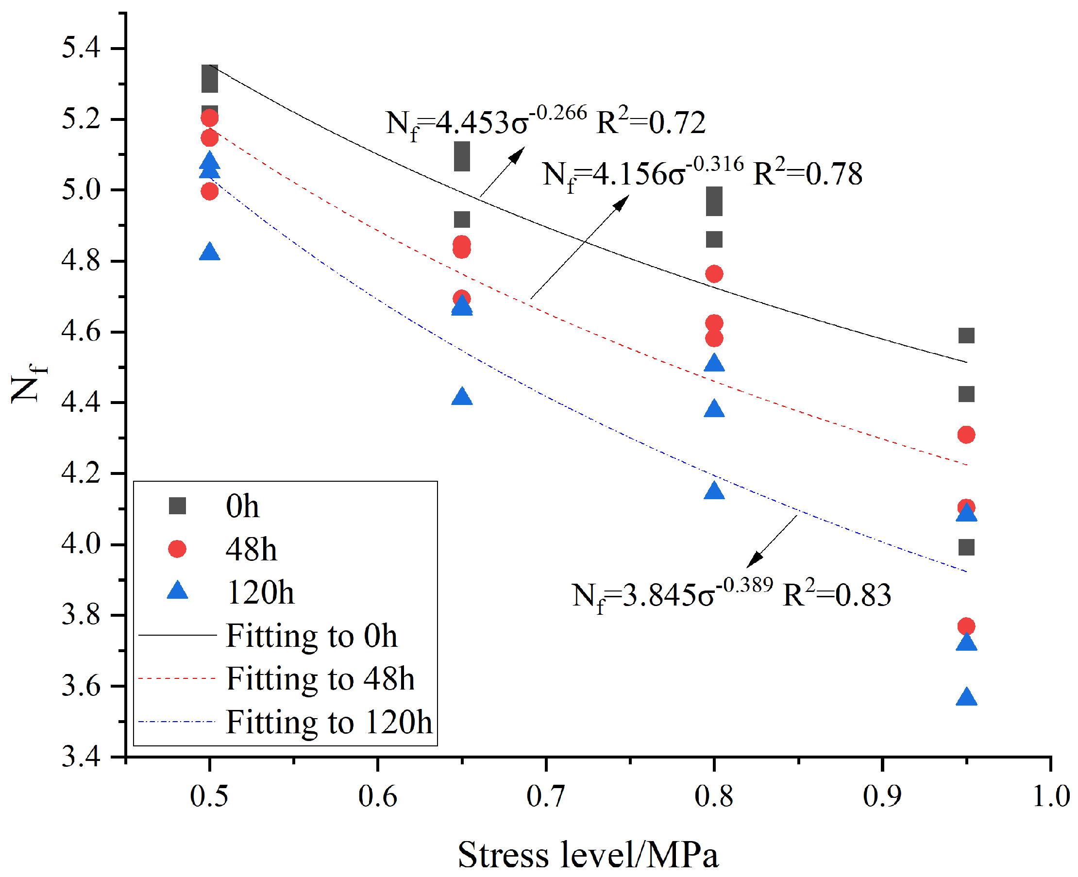
To determine the effect of immersing for different lengths of time on the fatigue life prediction model, the equation $N_f=c\ast {\sigma }^d$ was used to fit the related stress levels to the fatigue life of composite beams under different immersion time conditions. The result is shown in Figure 6. It is clear from the figure that shorter immersion times result in greater fatigue resistance in the samples. This indicates that the fatigue life of the specimen under this condition is more sensitive to stress levels. This is because water seeps into the barrier between the aggregate and the asphalt in the case of prolonged immersion of the specimen, thus reducing asphalt viscosity. Subsequent water damage to the specimens was exacerbated during the four-point bending fatigue test, leading to a decrease in the fatigue strength of the specimens. Since bitumen was used as the viscous oil in this study, the fatigue properties of the specimens are particularly susceptible to water damage.

(2)

Effect of different viscous layer oils on fatigue life prediction model parameters

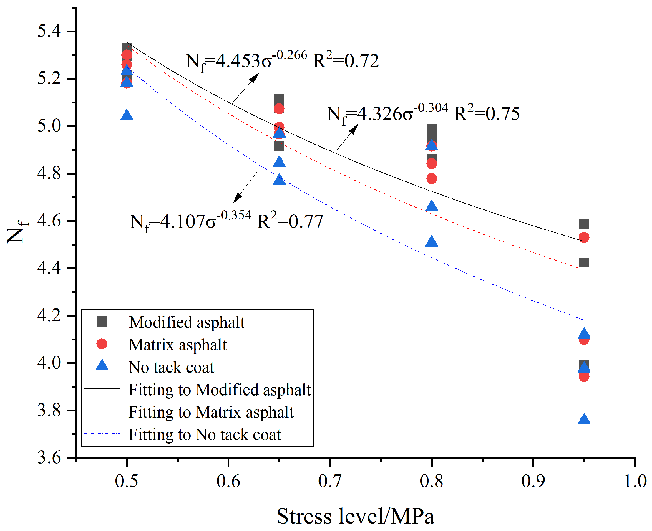
To evaluate the effect on the fatigue prognosis model of the different types of viscous layer oils, the variation rule of fatigue life with different viscous layer oils is shown in Figure 7. $N_f=c\ast {\sigma }^d$ was used to determine the connection between the life span and the stress level of the composite beams under different viscous oil conditions. Figure 7 shows that as the stress level increases, the fatigue of the composite beam sample subsequently decreases. The magnitude of the fatigue life span of the specimen of the compound beam with the different viscous layer oils is ranked under the same stress level: SBS-modified asphalt > 70# asphalt > no tack coat oil. This is mainly because the asphalt viscous layer oil is a viscoelastic material, which has a cushioning influence on crack propagation in the composite beam, making fatigue life even more fantastic. It is also possible to see that the fatigue resistance of SBS asphalt as a viscous layer oil is superior to that of 70# asphalt.

Establishing the relationship between the values of parameters c and d and different viscous oils is complex because the consistent amount of oil used in different viscous layers makes it difficult.

Therefore, we propose using the BISAR 3.0 interlayer friction parameter to precisely and quantitatively differentiate between different viscous layer oil values (e.g., Equation (2)) [36,37].

$$\partial ={\displaystyle \frac{AK}{AK+\frac{1+\nu }{E}\cdot r}}$$

(2)

where r is the load radius, m; E is the modulus of all layers above this layer, Pa; v is the Poisson’s ratio of this layer; AK is shear elastic compliance; $\partial$ is the friction parameter ($0\le \partial \le 1$). When $\partial$ = 0, the friction force is the largest. When $\partial$ = 1, the friction force is 0.

The simulations yielded 0.85, 0.56, and 0.13 for no tack oil, 70# asphalt, and SBS asphalt conditions, respectively.

(3)

Effect of different void fractions on fatigue life prediction model parameters

To determine the effectiveness of different void ratios on the fatigue life prediction model, $N_f=c\ast {\sigma }^d$ was used to fit composite beam fatigue life versus the stress level at different porosities, as shown in Figure 8. From the figure, it can be seen that at the same stress level, an increase in porosity leads to a reduction in fatigue life during the composite beam test. The rationale for this is that as the asphalt mixture void content increases, the surface area of its graded particles increases so that the layer thickness of asphalt on the particle surface is reduced for the same amount of asphalt. This reduction in bonding strength compromises the structural integrity, ultimately lowering the material’s strength and shortening its fatigue life.

(4)

Combined effects of different immersion times, viscous oil, and void fraction on fatigue prognostic modeling parameters

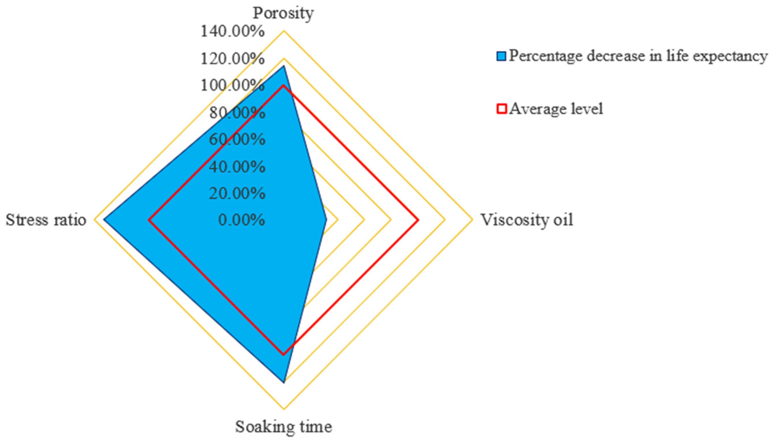
The impact of each factor on composite beam fatigue life is shown in Figure 9.

Figure 9 shows that the fatigue life of the composite beam decreased by 146% when the stress level increased from 0.5 to 0.95. The composite beam fatigue life decreased by 108% when porosity increased from 2.5% to 6%. The fatigue life decreased by 116% with immersion time increasing from 0 h to 120 h. The fatigue life of the viscous layer oil decreased by 29% when switching from SBS to matrix asphalt. Therefore, the stress ratio, porosity, and immersion time have a significant impact on composite beam fatigue, whereas the effects of viscous oil type on composite beams are not substantial. The more significant the stress ratio and the higher the porosity, the more serious the fatigue life of the composite beam decreases. The fatigue life of the composite beam decreases extremely fast when it is just immersed in water, and the decrease in fatigue life occurs slowly with increasing immersion time.

For the above values of a and b with different immersion times T, void ratio K, and viscous oil Y, a one-way fitting relationship has been established. Because a and b need to consider the three variables simultaneously on their influence law, it is assumed that the coefficients a and b of this fatigue equation satisfy the form as in Equation (3):

$$\left\{\begin{array}{c}a=P_1+P_{2}T+P_{3}Y+P_4{Y}^2+P_{5}K+P_6{K}^2\\ b=P_1+P_{2}T+P_{3}Y+P_4{Y}^2+P_{5}K+P_6{K}^2\end{array}\right.$$

(3)

where P₁, P₂, P₃, P₄, P₅, and P₆ are parameters.

This paper obtains all parameters of the composite beam fatigue life prediction model, as shown in

Table 3. The values for each parameter of the fatigue life prediction model.

Parameter	P1	P2	P3	P4	P5	P6
a	6.204	−0.004	−0.617	0.466	0.564	0.048
b	−0.5376	−0.0002	−0.202	0.164	−0.117	0.009

. By using the McQuarter iterative method and the generalized global optimization method in 1stOpt, the coefficients in Equation (3) are obtained.

The final fatigue life prediction model for the composite beam specimen under the combined influence of four factors, namely, different stress levels, immersion times, viscous layer oils, and void ratios, is obtained as follows:

$$\begin{array}{l}lg{N}_f=6.104-0.004T-0.617Y+0.466Y^2+0.564K+0.048K^2+\\ \left(-0.576-0.0002T^2-0.202Y-0.164Y^2-0.117K+0.009K^2\right)lg(\sigma )\end{array}$$

(4)

The software 1stOpt shows a correlation coefficient of 0.98.

3.2. Fatigue Damage Performance Evaluation of Composite Beams

Based on the four-point flexural fatigue testing of the composite beam specimen under water immersion for 48 h at four stress levels, three porosities, and three viscous layer oils, the fatigue modulus decay in Equation (5) [38] was fitted to derive the asphalt mixture composite beam modulus decay law under four different stress levels, three porosities, and three viscous layer oils, as shown in Figure 10.

$${\displaystyle \frac{E_{\mathrm{N}}}{E_0}}={\left[1-{\left({\displaystyle \frac{N}{N_f}}\right)}^m\right]}^n$$

(5)

where $E_N$ is the value of dynamic bending and tensile modulus for the Nth time of load application; $E_0$ is the initial bending modulus; $E_N/{\mathrm{E}}_0$ is the modulus ratio of the material when the load is applied N times; $N/N_f$ is the life ratio; m and n are the relevant material parameters.

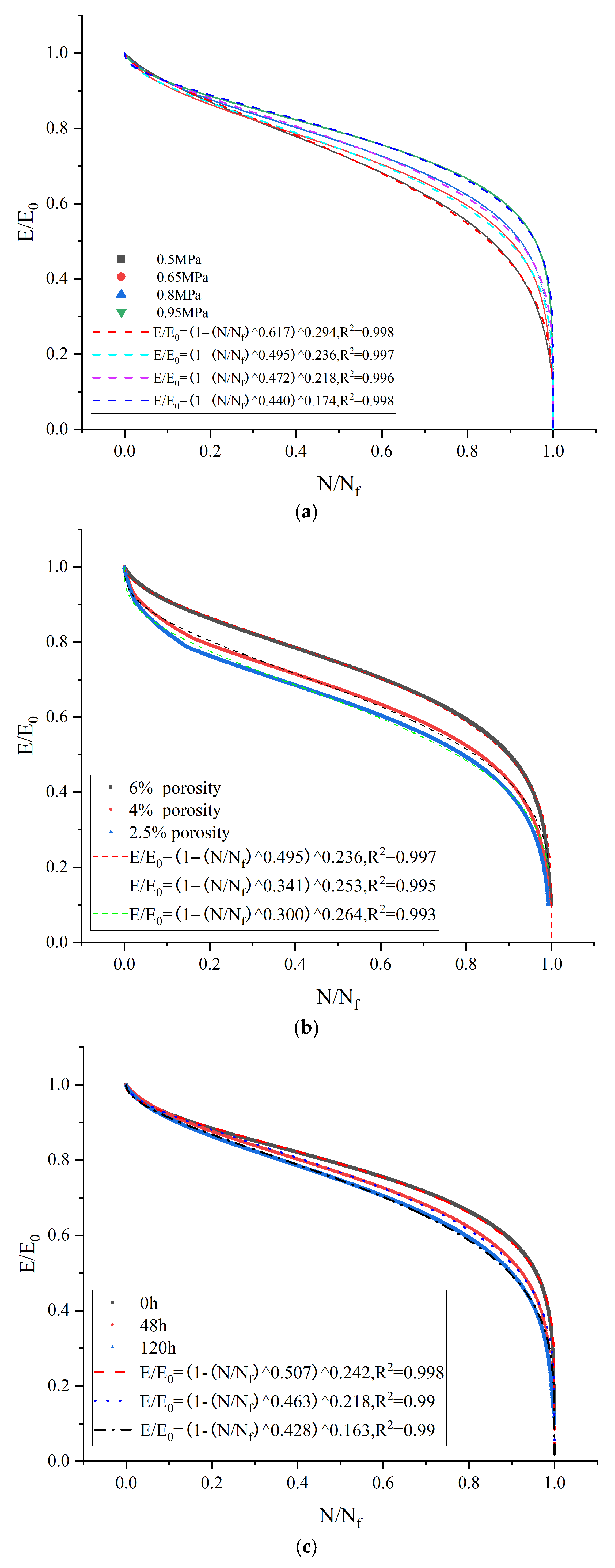
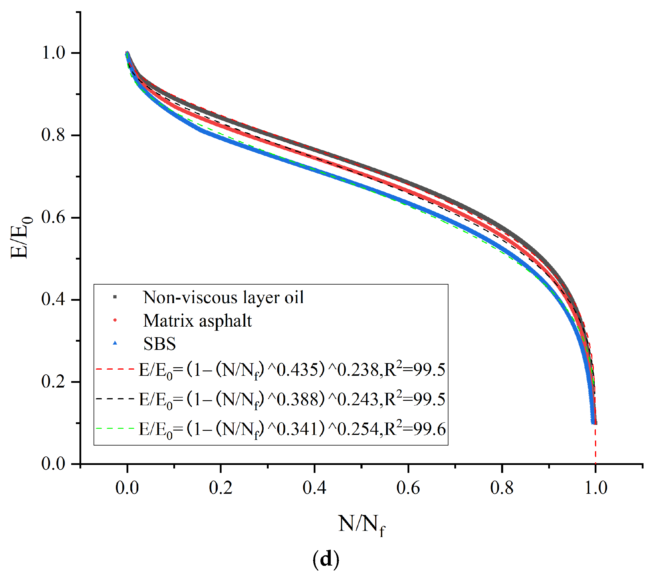
Figure 10 shows the modulus decay curves of a composite beam under different stress levels, porosity, and viscous layer oils. The general trend of these curves is similar, initially showing a rapid drop in modulus at the beginning of the life ratio. Then, the curves enter a phase of slow decrease, and finally, the rate of decrease accelerates further. In particular, the modulus decreases sharply when the life ratio reaches about 0.9. For the same life ratios, the higher the stress ratio and the higher the porosity of the composite beam specimen, the higher the position of the modulus curve. The modulus curve of the non-sticky layer oil is at the top, followed by the matrix asphalt sticky oil, while the SBS sticky oil is at the bottom of the modulus curve. Because the fatigue life and the viscosity of the viscous layer of oil material itself are closely related to the viscous asphalt, showing the longest fatigue life, the fatigue resistance is also the best.

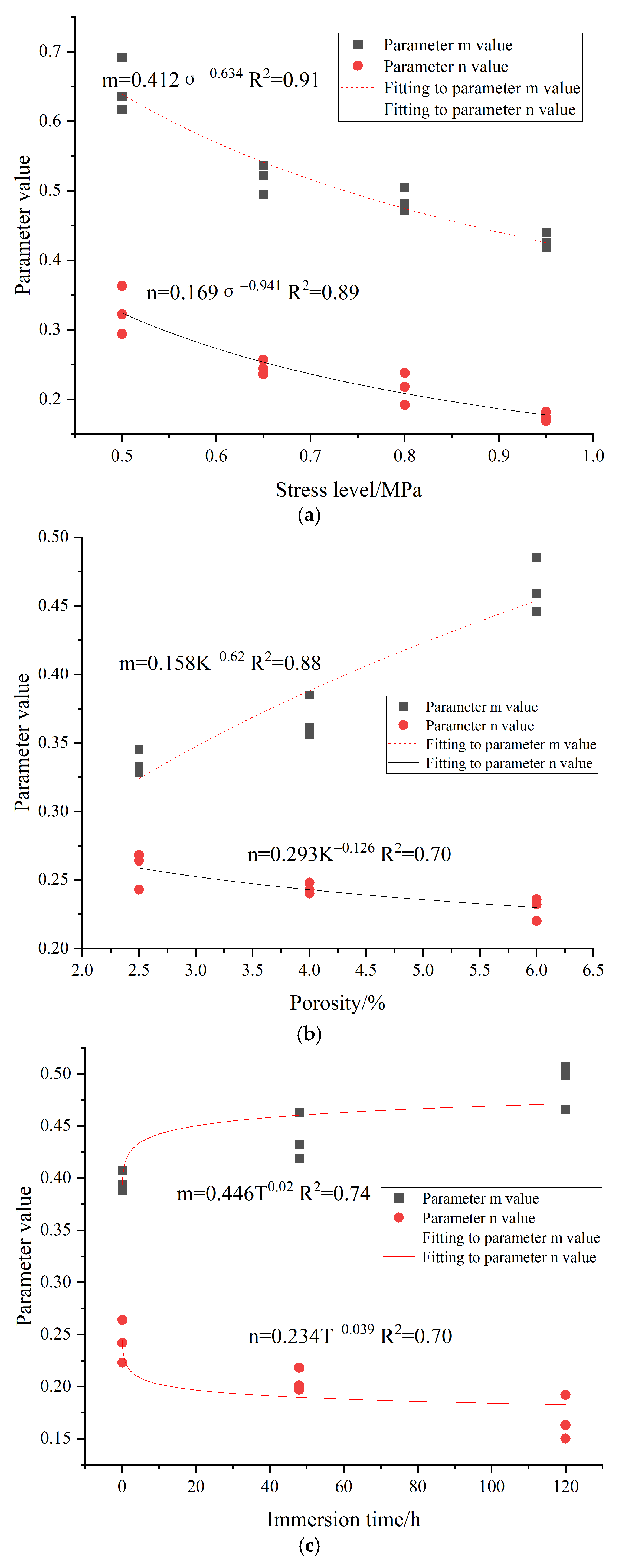
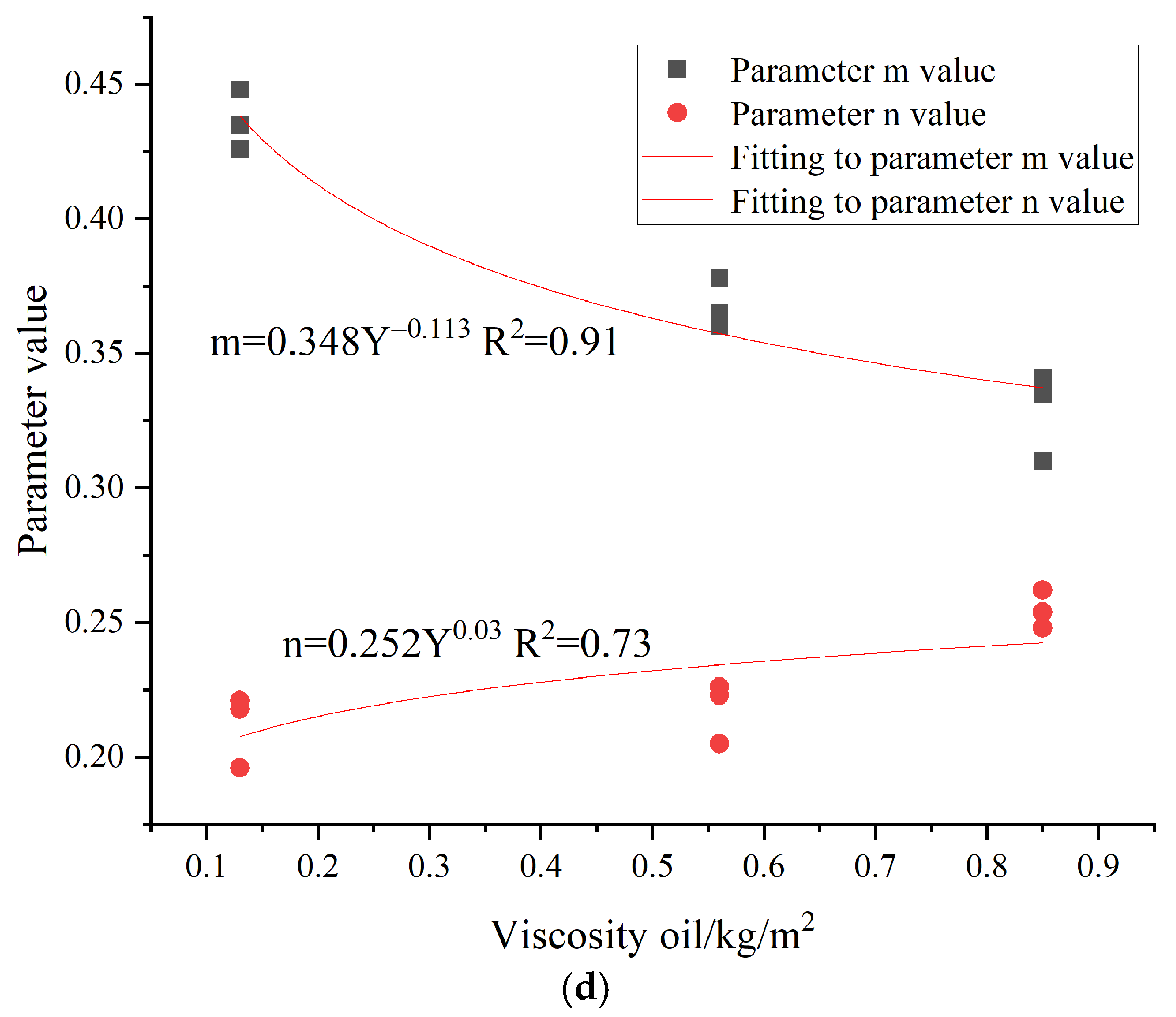
The decay curves of the lower modulus as a function of the lifetime ratio under the influence of various factors, fitted using Equation (5), are shown in Figure 10. It is visible that the function can effectively fit the decay law of the composite beam modulus, with a high correlation coefficient. The relationship between the modulus decay parameters m and n and the different influence factors is fitted as shown in Figure 11.

Since the evolution of the modulus decay parameters m and n with different influence factors is by the power function decay law, in order to investigate the effects on parameters m and n under the combined influence of different stress levels, porosity K, viscous layer oil Y, and water immersion time T, the following model can be established [37]:

$$m\mathrm{or} n=s{\sigma }^t{K}^u{Y}^v{T}^w$$

(6)

From the regression equations of parameters m and n under different stress levels, porosities K, viscous layer oils Y, and submergence times T, the parameters of Equations (6) and (7) are given in

Table 4. Values of each parameter of modulus decay for parameters m and n (regression model).

Parameter	s	t	u	v	w
m	7.49	5.5	4	−1.25	0.156
n	1.846	0.688	0.064	0.141	0.093

.

Therefore, the regression equations for the decay parameters m and n under the combined effect are as follows:

$$m=7.49{\sigma }^{5.5}{K}^4{Y}^{(-1.25)}{T}^{0.156}$$

(7)

$$n=1.846{\sigma }^{0.688}{K}^{0.064}{Y}^{0.141}{T}^{0.093}$$

(8)

For fatigue testing in stress-controlled mode, the complete fracture of the specimen is generally taken as the damage criterion. However, some researchers believe that the initial composite modulus of the specimen decreases to 90% of the material damage during standard stress fatigue testing. 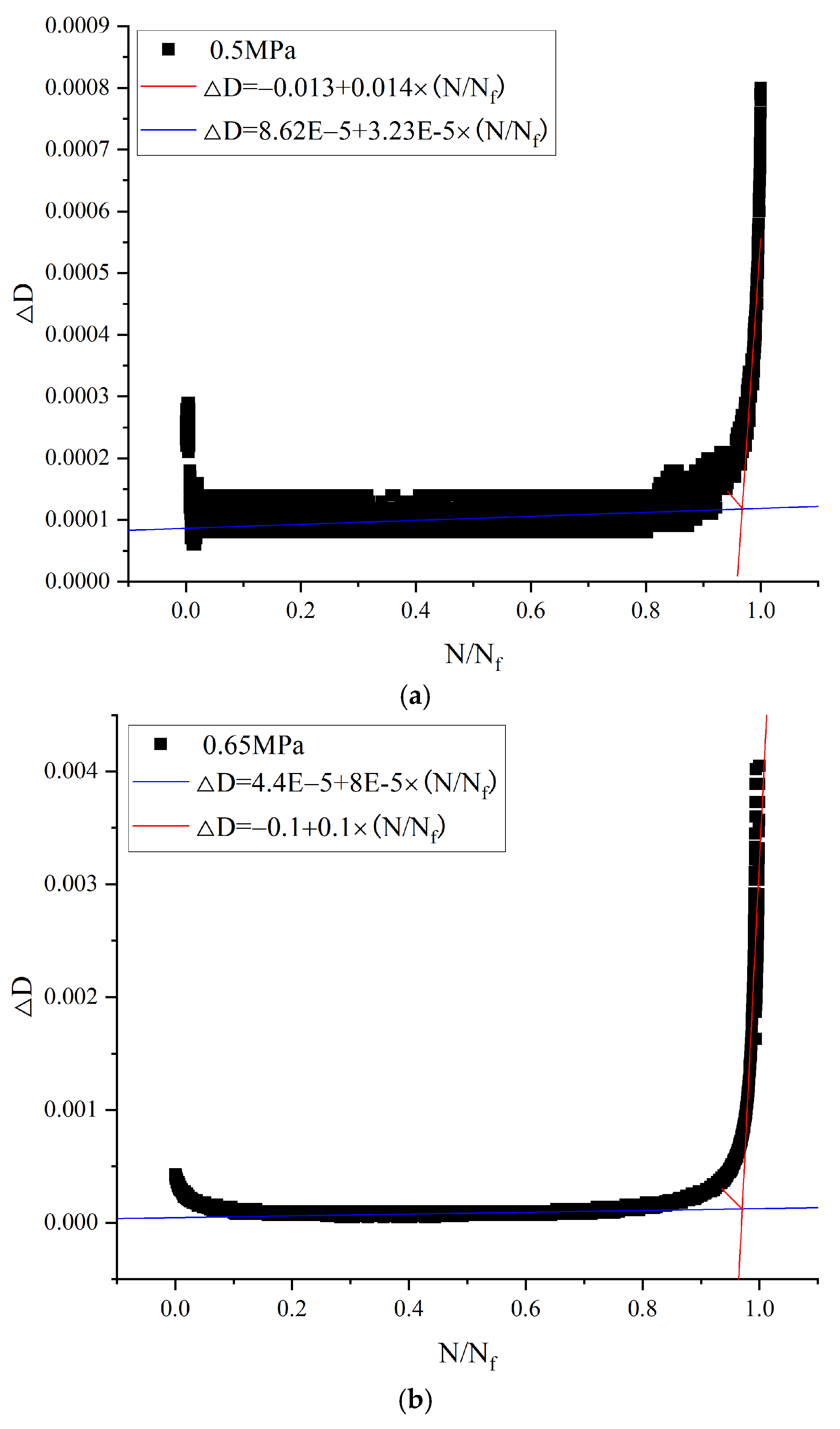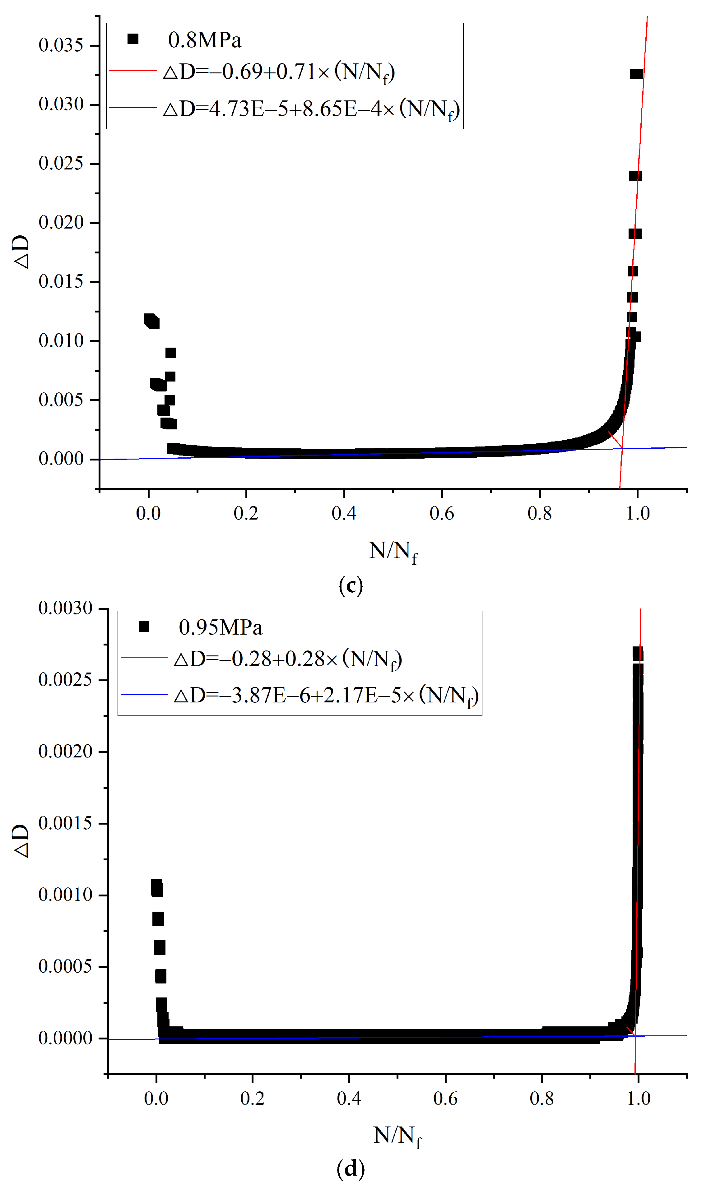Abo-Qudais, however, considers that the specimen fails when the strain value of the specimen reaches two times the initial strain [38]. These commonly used fatigue damage criteria are determined more arbitrarily. With a subjective element and due to the different criteria, the same asphalt mixtures exhibit different fatigue lives in fatigue tests using different loading patterns. From the curve of the damage factor increment ΔD versus the lifetime ratio N/N_f, the sharp increase in the damage factor increment during the accelerated damage phase of fatigue damage indicates the onset of damage to the specimen. Therefore, a sharp increase in the damage increment can be defined as a criterion for determining the fatigue damage of the specimen. The critical damage determination methodology is shown in Figure 12.

The damage corresponds to the angular bisector of the intersection of the fitted curves of the steady phase of damage increment, and the accelerated damage phase is the critical damage. The dynamic modulus is defined as the fatigue damage variable of the test sample. The critical failure equation derived is as follows [39]:

$$D_{cf}=1-{\displaystyle \frac{E_{min}}{E_0}}$$

(9)

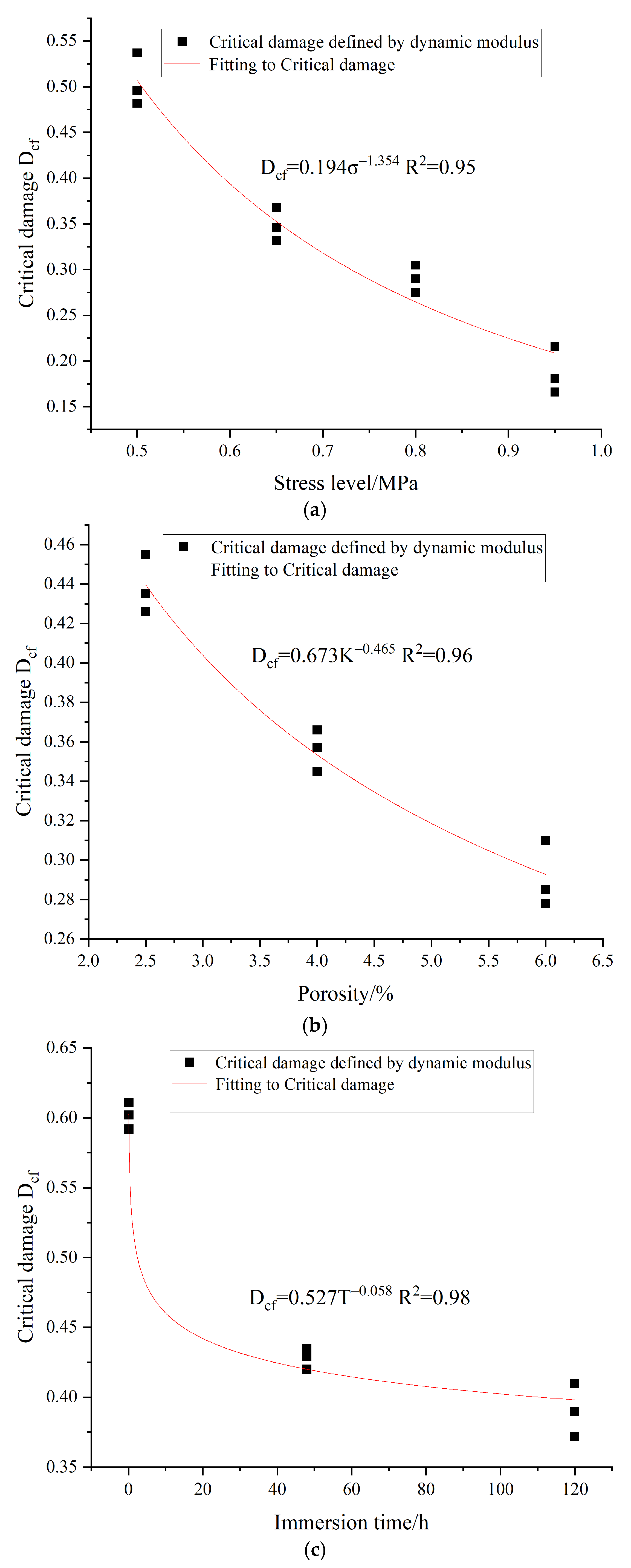
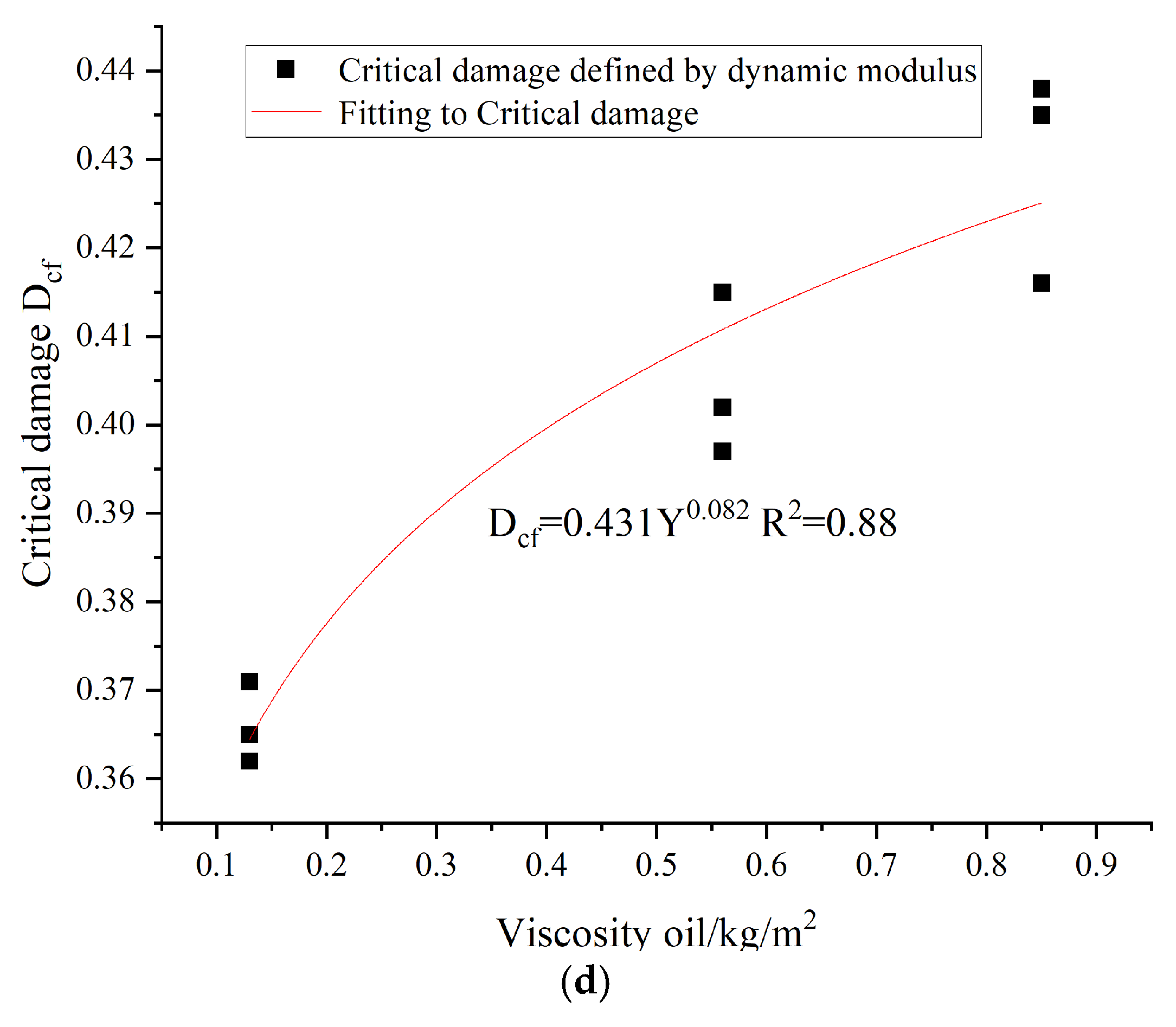
where D_cf is the threshold value of fatigue damage for defining fatigue damage variables based on the dynamic modulus; E_min is the momentum modulus value when the damage increment starts to grow sharply. The statistics of critical damage D_cf for each group of specimens depend on the fatigue damage criterion with a sharp increase in damage increment. The changing essential pattern of damage with different influence factors is shown in Figure 13.

Let the regression model of critical damage under the combined effect of different factors be as follows:

$$D_{cf}=s{\sigma }^t{K}^u{Y}^v{T}^w$$

(10)

From the regression equation of critical damage D_cf under the effect of various factors, the values of each parameter in Equation (10) can be derived, as can be seen in

Table 5. Values of each parameter of the critical damage D_cf regression equation.

Parameter	s	t	u	v	w
Values	0.528	−1.688	1.375	−0.113	−0.154

.

Therefore, the regression equation for the critical destructive force D_cf under the influence of different factors is as follows:

$$D_{cf}=0.528{\sigma }^{-1.688}{K}^{1.375}{Y}^{-0.113}{T}^{-0.154}$$

(11)

Considering a dynamic modulus of the damage and the effect of critical damage combined with the decay model of the dynamic modulus function, the following nonlinear dynamic modulus decay-based fatigue damage modification model is established.

$$D_f(N)=1-{\displaystyle \frac{E}{E_0}}={\displaystyle \frac{(E_0-E_{\min }){[1-{(\frac{N}{Nf})}^m]}^n+E_{\min }}{E_0}}=D_{cf}[1-{(1-{({\displaystyle \frac{N}{N_f}})}^m]}^n$$

(12)

Substituting Equations (7), (8), and (11) into Equation (12) yields the following nonlinear fatigue damage equation under the combined effect of multiple factors:

$$\begin{array}{l}{D}_f\left(N\right)=(0.528{\sigma }^{-1.688}{K}^{1.375}{Y}^{-0.113}{T}^{-0.154})\\ {{[1-{(1-({\displaystyle \frac{N}{N_f}})}^{7.49}{\sigma }^{5.5}{K}^4{Y}^{-1.25}{T}^{0.156}]}^{1.846}}^{{\sigma }^{0.688}{K}^{0.064}{Y}^{0.141}{T}^{0.093}}\end{array}$$

(13)

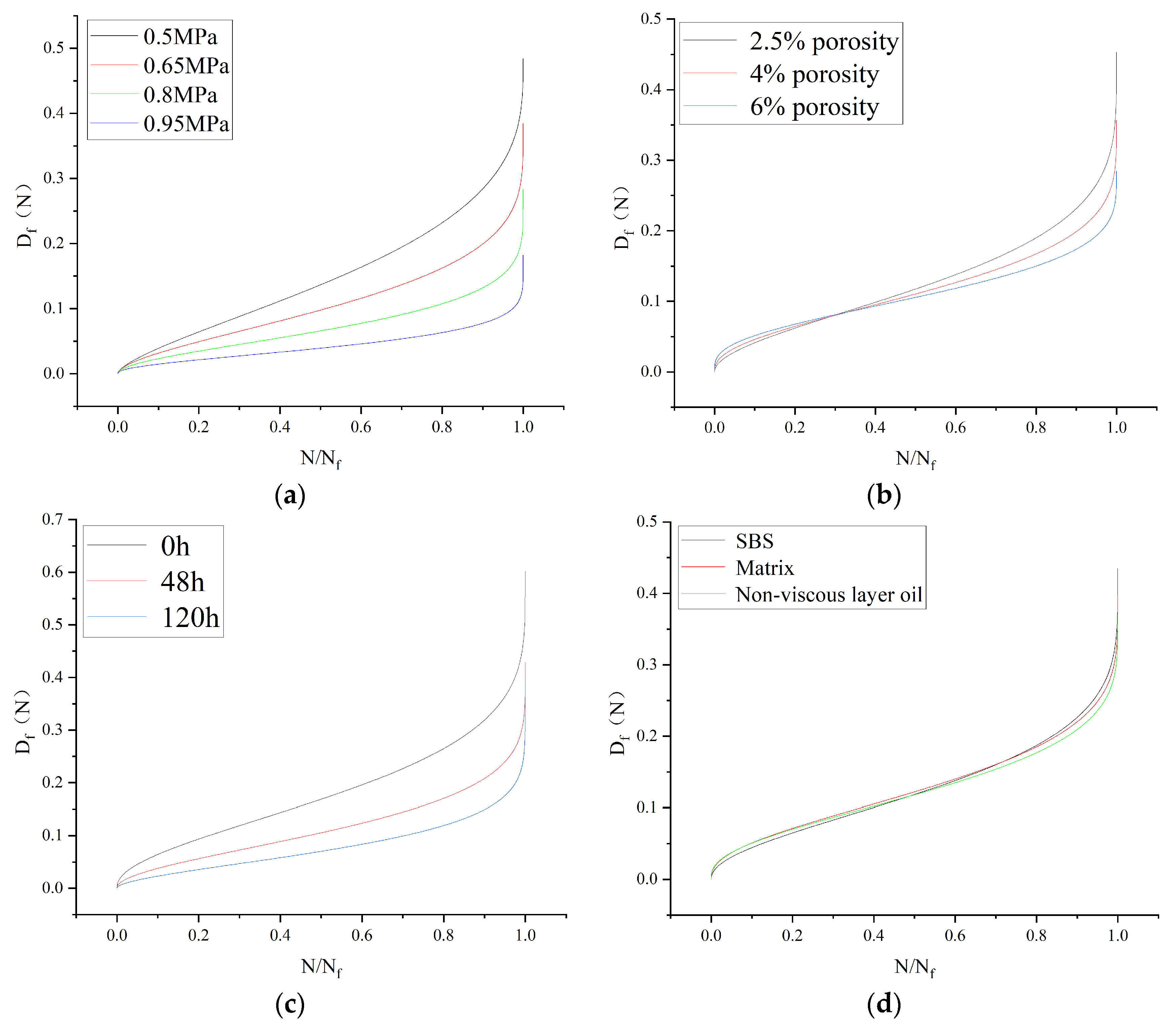
From Equation (13), the evolution of the damage D_f(N) based on the definition of the dynamic modulus for different stress levels, porosity, viscous oil, and water immersion time can be derived, as shown in Figure 14.

From Figure 14, it is clear that fatigue damage grows slowly at the beginning of the life ratio of the composite beam, then accelerates with the increase of the life ratio, and rises sharply in the later stage. The critical fatigue damage under different stresses also varies. The damage corresponding to a life ratio of 1 in Figure 14 represents the critical fatigue damage for a load. Fatigue damage curves under stress levels of 0.5 MPa, 0.65 MPa, 0.8 MPa, and 0.95 MPa are shown in Figure 14a from top to bottom, indicating that higher stress levels result in smaller critical fatigue damage in composite beam specimens. From Figure 14a–c, it can be seen that the larger the porosity and stress ratio, and the longer the immersion time, leading to smaller critical fatigue damage to the composite beam specimens. Thus, the higher the stress level, the greater the porosity, and the longer the immersion time, the greater the damage caused by the last fatigue. From Figure 14d, it is apparent that the critical damage of SBS viscous oil is the largest, while that of non-viscous oil is the smallest, with matrix asphalt in the middle. However, the fatigue damage curves for different viscous oils are closely aligned, suggesting that the type of viscous oil used as a binder layer has only a minor impact on the fatigue behavior of the composite beam specimens.

3.3. Study on Crack Propagation of Specimens Based on DIC Technology

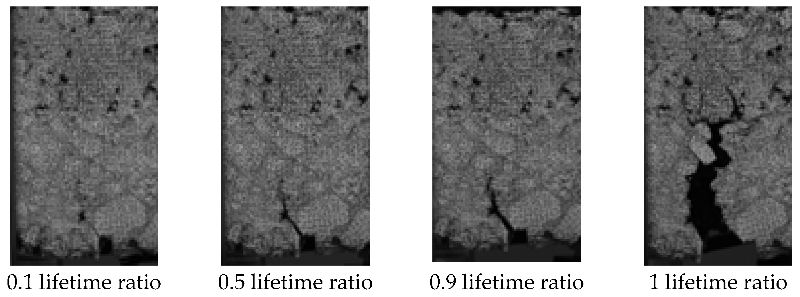
The horizontal displacement of the crack is obtained based on the DIC technique to get the fatigue crack length L of the composite beam under different numbers of load cycles N_f. Taking 0.65 MPa as an example, the crack extension process of the specimen is shown in Figure 15. The crack length L is calculated as the initial value at the top of the prefabricated cracking, which is the worth of the crack length at the maximum stress corresponding to a specified number of cycling. Additionally, the maximum crack width w_max refers to the value of the largest cracking width for the maximum stress corresponding to a certain number of cycles.

Figure 16 and Figure 17 represent the connection between the length, width, and fatigue life span of compound beam specimens under different influence factors. In this paper, the logistic function [40] functional form is used to fit the L~N_f curve, which is expressed as follows:

$$L=\mathrm{f}\ln ({\displaystyle \frac{g-N}{hN-ge}})$$

(14)

where L is the length of the crack; N is the fatigue life; and e, f, g, and h are the fitting parameters. Analyzing the parameters for each condition, it was found that the value of the parameter e tends to be −1, irrespective of the condition of the specimen. So, we set e in Equation (15) to −1 as follows:

$$L=\mathrm{f} \ln ({\displaystyle \frac{g-N}{hN+g}})$$

(15)

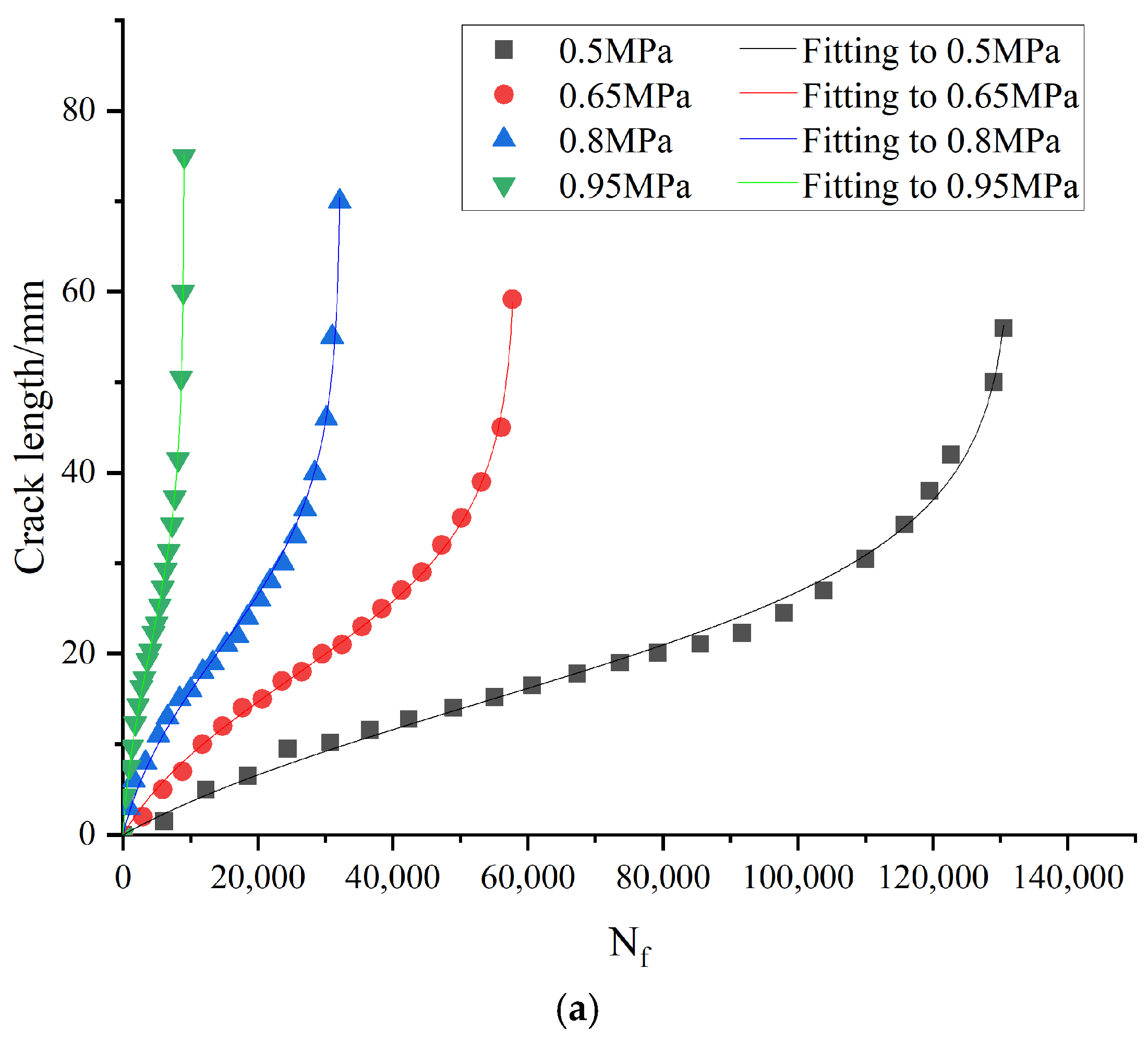
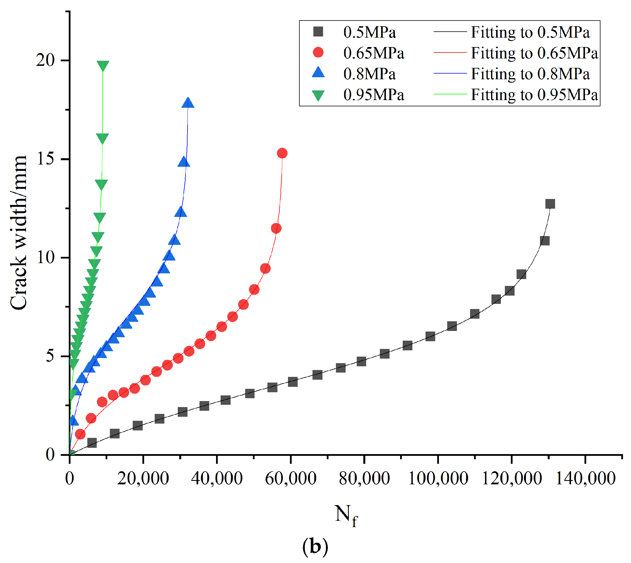
Figure 16 and Figure 17 show the fitting with Equation (15), and the fitting parameters are shown in

Table 6. Fitting parameters of crack length and fatigue life under different conditions.

Fitting Parameters	f	g	h	R2
0.5 MPa	−8.93	131,931	5.12	0.984
0.65 MPa	−8.68	58,298	7.47	0.988
0.8 MPa	−9.34	32,298	8.91	0.984
0.95 MPa	−9.29	9079	9.12	0.985
2.5%	−9.78	102,068	5.34	0.979
4%	−7.26	71,027	10.78	0.972
6%	−9.32	53,139	11.02	0.982
Non-viscous layer oil	−8.95	45,829	11.18	0.974
Matrix asphalt	−9.19	60,446	7.35	0.981
SBS	−8.70	65,467	7.54	0.983

and

Table 7. Fitting parameters of crack width and fatigue life under different conditions.

Fitting Parameters	f	g	h	R2
0.5 MPa	−2.04	132,225	5.22	0.988
0.65 MPa	−1.90	57,964	11.45	0.987
0.8 MPa	−1.93	32,244	37.4	0.975
0.95 MPa	−1.86	9065	65.6	0.986
2.5%	−1.73	101,328	28.88	0.98
4%	−1.69	72,903	37.4	0.975
6%	−1.99	52,980	29.96	0.974
Non-viscous layer	−1.88	45,725	32.13	0.983
Matrix asphalt	−1.76	60,195	35.56	0.979
SBS	−1.63	65,123	31.89	0.949

. The correlation coefficients obtained from the fitting are all above 98%. This indicates that this equation better fits the relationship between cracking and the fatigue life of composite beam specimens with different stress ratios, porosities, and viscous layer oil conditions compared to Equation (14).

From Figure 16 and Figure 17, it is evident that the bending fatigue cracking process of composite beams is similar to that of an ordinary beam. Both exhibit a clear three-stage progression of fatigue life and crack development: crack initiation, steady propagation, and unstable expansion. Initially, stress concentration at the pre-existing cracks located at the bottom span of the composite beam triggers crack formation, which then propagates rapidly.

When the stress ratio is 0.65, it is apparent from Figure 16 that at this stage, the cracking length of the composite beam specimen reaches 7 mm and the width reaches 2.68 mm after 8845 cycles of loading. This is due to the fact that the asphalt mixture specimen itself continues to self-adjust and densify under loading, accompanied by the initiation of microcracks. This results in a significant increase in vertical displacement, marking the crack initiation stage. However, the duration of this stage is relatively short, with the number of load cycles accounting for less than 15 percent of the entire fatigue life.

As cyclic loads continue to be applied to the composite beam, the crack extends to the bottom of the upper layer, while the bottom has not developed cracks at this point. Therefore, the overall crack expansion of the composite beam enters a slow and stable expansion stage. At this stage, the number of cycles of the composite beam specimen increases from 8845 to 53,134 as the fatigue crack length increases by about 32 mm and the width increases by about 6.77 mm. At this stage, internal changes in the specimen’s stabilized, horizontal strains are concentrated at the bottom of the beam and continue to accumulate causing microcracks within the material to converge into large cracks and expand steadily, with the number of load cycles accounting for 77% of the entire fatigue life.

The growth of fatigue cracks before specimen failure leads to a significant decrease in stiffness, which affects the overall performance of the asphalt mixture composite beam. As the cyclic load continues to be applied, the material becomes unable to withstand the established load, rapidly deforming and causing the macroscopic crack to expand quickly to specimen fracture. The fatigue crack length of the specimen extends from 39 mm to 59 mm at this stage; composite beam rigidity decreases rapidly, resulting in specimen failure. The fatigue crack length of this stage constitutes less than 7% of the total life.

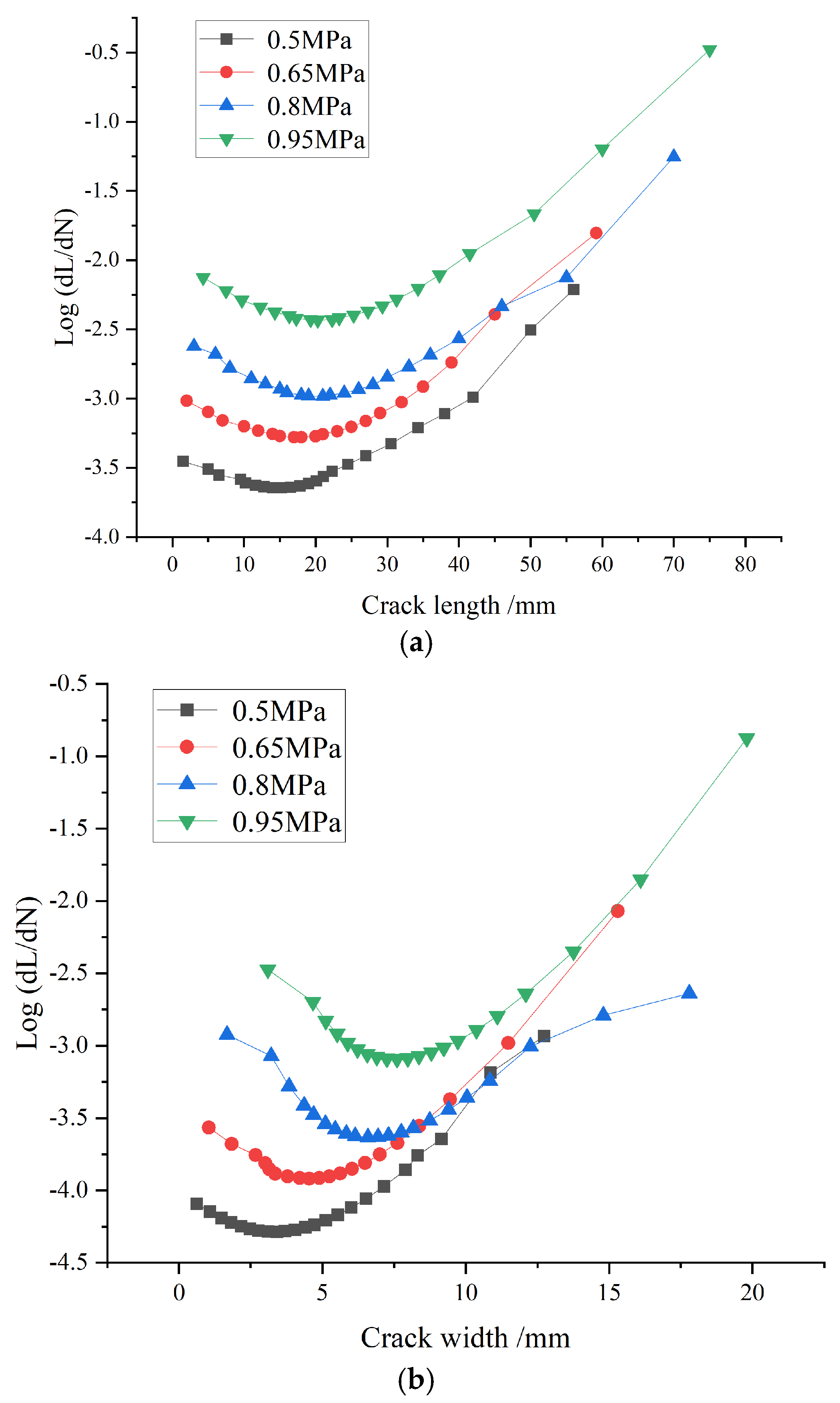
The crack extension rate can be calculated by the first-order derivative of Equation (16):

$${\displaystyle \frac{dL}{dN}}={\displaystyle \frac{g(h+1)f}{(g-N)(-g-hN)}}$$

(16)

The relationship between crack growth rate and crack length (width) at different stress levels is shown in Figure 17. The critical crack length (width) Lc can be obtained by making the second-order derivative of Equation (16) zero as in Equation (17). The critical life N_c can also be obtained as in Equation (18):

$$L_{\mathrm{c}}=2 f \ln (1/h)$$

(17)

$$N_{\mathrm{c}}=g(h-1)/h$$

(18)

The critical crack length values at each stress are shown in

Table 8. Critical cracks and fatigue lifetimes at different stresses.

Stress Level	0.5 MPa	0.65 MPa	0.8 MPa	0.95 MPa
Length value	29.17	34.91	40.86	43.00
Width value	6.74	9.26	11.98	13.56
Critical life $N_{\mathrm{c}}$	106,163	50,494	28,673	8182
Fatigue life N	130,462	57,740	32,130	9051
$N_{\mathrm{c}}/N$	0.81	0.88	0.89	0.90

. From Table 8, it can be seen that the critical crack length (width) of the specimen increases when the stress level increases, with a consequent decrease in critical life. This is consistent with the general assumption. This could be a result of pre-cutting the seam, which leads to the idealized expansion of the crack on the specimen. The critical crack length (width) varies considerably with different stress levels. This difference affects the overall fatigue behavior of the specimen because the fatigue life of specimens subjected to higher stress levels is shorter.

Figure 18 shows that the minimum crack extension rate at different stress levels is the critical crack length (width) at that level. It is the transition from smooth to destabilized crack expansion. From this figure, it can be seen that the lower the stress level, the lower the crack extension rate of the specimens, which is consistent with their longer fatigue life.

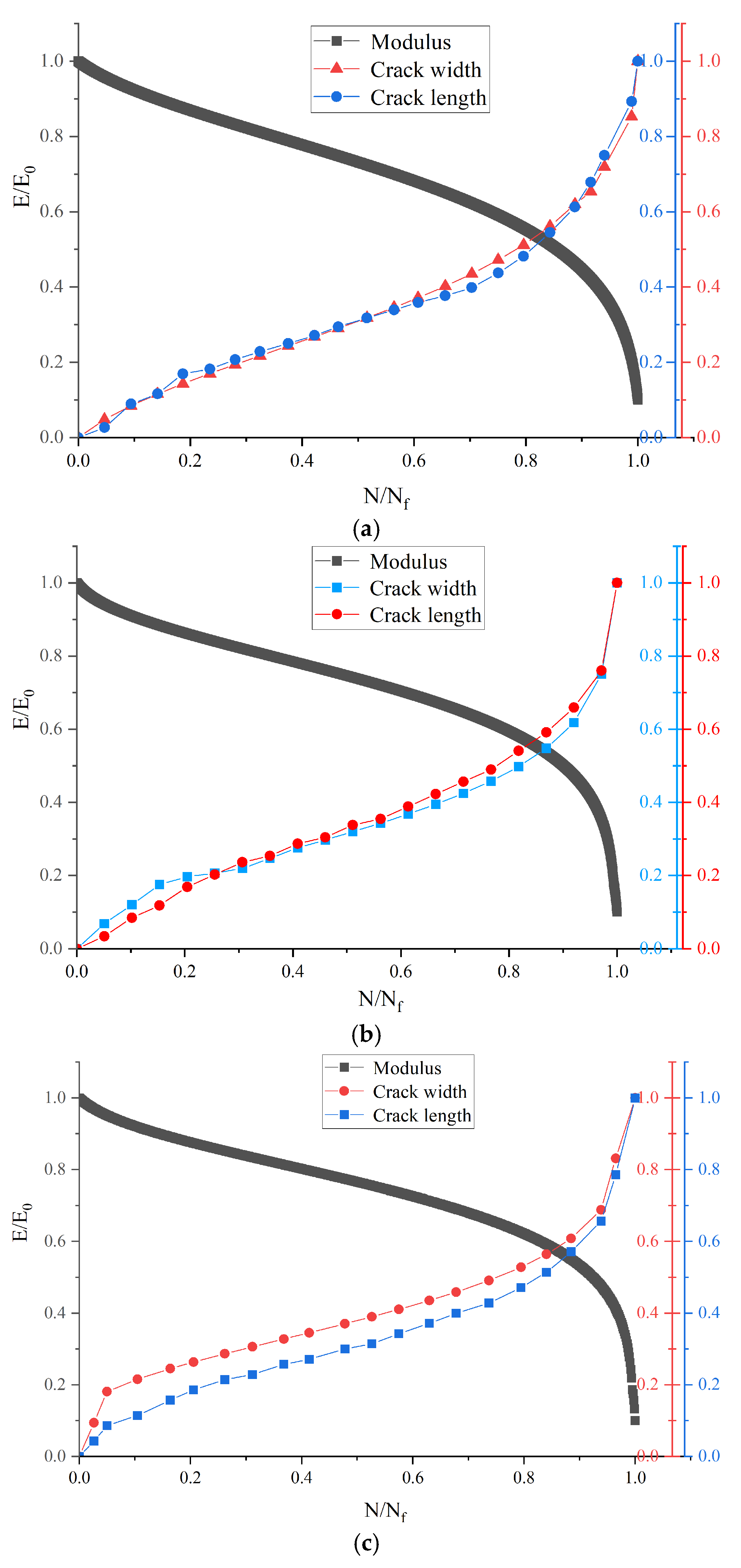
The stiffness ratio, crack length, and crack width are normalized as shown in Figure 19. It shows that both the crack width and length of composite beams increase as the life ratio grows under different stress levels, while the modulus decreases as the cracks expand. The decrease in the modulus of the composite beam is related to the crack expansion rate: the quicker the crack expansion rate, the faster the reduction in the modulus. When the crack expansion rate tends to stabilize, the rate of decrease in modulus also tends to stabilize.

The composite beam modulus and crack extension curves form an intersection as the life ratio increases. The modulus ratios at the intersections of the composite beam specimens at 0.5, 0.65, 0.8, and 0.95 MPa were 0.54, 0.54, 0.55, and 0.56. The life ratios were 0.81, 0.86, 0.88, and 0.91, and this is very close to the thresholds calculated in Table 8. Therefore, this point can be considered as the critical point of transition from smooth to unstable crack extension, while the modulus ratio of the inflection point is around 0.55, regardless of the stress level.

The modal attenuation at this point was calculated to be 45% by the field-measured modulus method [41,42]. As seen in Figure 19, after this point, the rates of crack propagation and modulus reduction accelerate noticeably. Therefore, this point is identified as the transition from a stable to an unstable state in the composite beam specimen. It is recommended that asphalt pavements, after milling and resurfacing, should undergo timely major and intermediate repairs before the modulus decay reaches 45%.

4. Conclusions

In this study, four-point bending fatigue tests were conducted on composite beams made from pre-cut seam asphalt mixtures, examining the effects of varying stress ratios, immersion times, viscous layer oils, and void ratios. The fatigue crack propagation on the surface of asphalt mixture composite beams was observed using digital image correlation techniques, and the following conclusions were obtained:

• Fatigue prediction equations were developed using the stress level, immersion time T, void ratio K, and viscous oil Y as independent variables. These equations reflect the rule of change in the fatigue life of asphalt mixture composite beams under the combined influence of the four variables: T, K, Y, and the impact of different factors on the fatigue life of composite beams. Porosity, stress ratio, and immersion time significantly affect the fatigue life of composite beam specimens. The effect of different viscous layer oils on the fatigue life of composite beam specimens was not significant. The prognostic model integrates the influences of stress level, soak time, void ratio, and viscous oil. More accurately predicting fatigue life can reduce damage to asphalt pavements after milling and resurfacing due to fatigue damage and improve the performance and safety of the pavement.
• By defining the dynamic modulus as a damage variable under multiple factors, a nonlinear fatigue damage model for the critical fatigue behavior of composite beams was developed. The model describes how fatigue damage evolves nonlinearly when affected by stress level, immersion time, void ratio, and viscous layer oil. The damage pattern of reflection cracks on milled and resurfaced asphalt pavements under the influence of multiple factors was clarified.
• A modified logistic function model was developed to describe the crack extension and fatigue life span of compound beam samples under varying stress ratios, porosities, and viscous layer oil conditions. The composite beam modulus decreases with crack extension at various stress levels, and the decrease rate is proportional to the crack extension rate. It was statistically found that the modulus decay curves and crack extension curves of composite beams under different stress levels form an intersection point with the increase of the life ratio. At this critical point, the modulus ratio stabilizes around 0.55, marking the transition from a stable state to rapid crack growth and a sharp decline in the modulus, leading to specimen failure. Repairing before the modulus reaches this critical point reduces damage and the number of repairs, resulting in lower maintenance costs and improved economics.

This research enhances the understanding of the fatigue damage characteristics of the composite structural layer of asphalt pavement after milling and resurfacing. It provides a theoretical foundation for optimizing asphalt pavement structures and materials after milling and resurfacing. However, this study does not address the impact of temperature, fuel consumption, frequency, etc., on the fatigue performance of composite beams and the analysis of stress–strain cloud diagrams of composite beams under DIC. Future research will carry out bending fatigue tests of composite beams at different frequencies and temperatures and produce stress–strain maps and stress–strain curves of asphalt mixture composite beams analyzed by different fatigue test methods combined with DIC.