Bayesian Inference and Condition Assessment Based on the Deflection of Aging Reinforced Concrete Hollow Slab Bridges

Abstract

This paper presents a Bayesian inference framework for updating the structural rigidity ratio of aging hollow slab RC bridges using deflection measurements. The framework models the structural rigidity ratio as a stochastic field along the hollow RC slabs, using the Karhunen–Loeve (KL) transform to capture spatial correlation and variation. Bayesian inference is then applied using deflection data from static loading tests, supported by a finite element model (FEM) and a Kriging surrogate model to enhance computational efficiency. The posterior distribution of the structural rigidity ratio is derived using a Markov chain Monte Carlo (MCMC) sampler. The proposed method was tested on an RC bridge with hollow slabs, using deflection measurements taken before and after reinforcement. The Bayesian updates indicated increased structural rigidity ratios after reinforcement, validating the effectiveness of the reinforcement. The deflection predictions from the updated models closely matched the measurements, with the 95% confidence bounds encompassing most of the data. This demonstrates the method’s validity and robustness in capturing the structural improvements post-reinforcement.

1. Introduction

Reinforced concrete (RC) bridges constitute a significant portion of China’s bridge network. By the end of 2022, the country’s roadway network included 1,033,200 in-service bridges, with RC bridges accounting for 80% to 90% of the total [1]. Primarily constructed during the 1980s and 1990s, these aging bridges have undergone varying degrees of degradation due to continuous exposure to environmental stressors and repeated impacts, significantly affecting their structural safety and serviceability. Consequently, the financial burden of maintaining these aging bridges has become a major concern. This increasing cost of bridge maintenance is a challenge faced by many countries [2], underscoring the global need for effective bridge management strategies. Therefore, efficient bridge management systems should be established based on accurate condition assessments of critical bridges in the network. This approach allows for the optimization of maintenance routines and better allocation of limited maintenance budgets, marking a transition from prescribed periodical maintenance to condition-based maintenance strategies [3,4,5,6,7,8,9,10,11,12].

The rapid development of structural health monitoring systems in recent years has provided bridge engineers with a substantial amount of data, enabling the estimation of the structural identification of bridges [13]. Structural identification of aging bridges is conducted using various dynamic indicators, including structural frequency [14], mode shape [15], modal curvature [16], strain mode [17], and structural flexibility [18]. These dynamic indicators have been shown to be damage-sensitive, and changes in these indicators are expected to suggest structural damage.

On the other hand, static indicators such as deflection have been used for the structural identification of aging bridges [18]. Theoretically, bridge deflection is correlated with multiple variables associated with structural safety and serviceability, including damage, structural rigidity, prestress loss, creep, and shrinkage. Therefore, structural identification based on bridge deflection can reveal the actual states of these variables. Furthermore, compared with dynamic indicators, static deflection excels in its low cost and better availability, as such data are readily available during the routine inspection of bridges [19]. Additionally, the measurement of deflection is subject to less noise compared to the measurements of dynamic indicators [20].

The current literature discussing structural identification using bridge deflection is mostly output-only analysis, which directly works on deflection data to extract damage-sensitive indicators [21]. One crucial issue in relevant studies is filtering out deflections caused by environmental factors, which involves establishing empirical input–output relationships between these factors and the corresponding deflections. In the method proposed by Peeters and De Roeck [22], the long-term deflection is divided into “normal” components under environmental influences such as wind loads and temperature, and anomalies caused by damage, considering the former not to be safety-affecting factors. Hedegaard et al. [23] identify anomalies in deflection from both short-term and long-term perspectives. In similar studies, the relationship between environmental factors and deflection increments is assumed to be linear or non-linear, and filtering techniques such as principal component analysis (PCA) and kernel principal component analysis (KPCA) are used to remove the environmental impacts [24].

As an alternative approach, model-based structural identification based on bridge deflection uses information from mechanistic models (e.g., finite element model, FEM) as well as deflection measurements to calibrate associated structural state variables. Results indicate that model-based structural identification using bridge deflection can outperform methods based on dynamic indicators. This advantage primarily arises from the stability of deflection measurements, which also eliminates the influences of structural mass and damping [25,26]. In a series of studies by Sanayei [25,26,27,28,29], the stiffness of elements in FEM is calibrated based on deflection measurements. Banan [30,31] formulates the inversion analysis into a least squares problem that minimizes the differences between measured static displacements and model predictions. The authors solved the optimization using the Monte Carlo method and discussed the influence of initial values on the solution results.

Beyond these deterministic methods, probabilistic structural identification methods are proposed based on Bayesian inference. Compared with deterministic methods, probabilistic structural identification using Bayesian inference can update the range of structural state variables while considering their uncertainties. The range estimation in the probabilistic method is more robust than the point estimation in the deterministic method, considering the stochastic nature of the structural state variables [32,33]. Nettis et al. [34] propose an automated framework for efficient probabilistic structural assessment of bridges, considering various critical corrosion scenarios and uncertainties in geometric and mechanical properties.

In this paper, the damage states of aging hollow slab bridges are subject to Bayesian inference using the deflection measurements collected during a static loading test. The damage states are defined by the distribution of the structural rigidity of the slabs, which are modeled as stochastic fields along the lateral direction of the bridge. A 3-D FEM is constructed to compute the deflection under various loading conditions. To improve the computation efficiency, a Kriging surrogate model of the FEM is trained and used as the forward model in the Bayesian inference. The posterior distribution of damage states is approximated by a Markov chain Monte Carlo (MCMC) sampler.

The remainder of this paper is organized as follows: Section 2 presents the methods of this paper, in which Section 2.1 presents the general procedures of the Bayesian inference considering the stochastic field of damage for aging hollow slab bridge; Section 2.2 presents the details of the setup of FEM and its Kriging surrogate model; Section 2.3 formulates the MCMC sampler used to derive the posterior distribution of the damage states. Section 3 presents a numerical application of the proposed method on an existing RC hollow slab bridge, using the deflection measurements from the field test.

2. Materials and Methods

2.1. Stochastic Field of the Damage States of Hollow Slab Bridge

Considering a hollow slab bridge, the structural damage states are represented by a set of random variables d = (d₁, d₂…d_N)^T. As shown in Figure 1, d_i denotes the ratio between the effective and nominal flexural stiffness of the i-th slab girder, i.e.,

$$d_i=E{I}_i/E{I}_{0i}$$

(1)

where EI_i and EI_0i are the effective and nominal flexural stiffness of the i-th slab girder, respectively. N denotes the number of slabs in the bridge.

In practical applications, d is often considered as a stochastic field. This approach takes into account the spatial correlation of damage, thereby preventing excessive variability in damage on adjacent hollow slabs, which is a common scenario in engineering projects.

In this paper, d is considered a one-dimensional stochastic field along the lateral direction of the bridge using the KL transform, which aims to reduce the dimensionality of a dataset while preserving as much variability as possible. It achieves this by transforming a set of correlated variables into a set of uncorrelated variables called principal components, ordered by the amount of variance each can explain. Then, d is derived as [35] the following:

$$d=d_{0}1+{\displaystyle \sum _{m=1}^N{\theta }_m}\sqrt{{\lambda }_m}{f}_m$$

(2)

where d₀ denotes the average damage of the slabs of the bridge; ${\lambda }_m$ and $f_m$ are the m-th eigenvalue and eigenvector of the autocorrelation matrix R, which are derived by the singular decomposition of R:

$$Rf=\lambda f$$

(3)

Here, the autocorrelation matrix R is derived using the autocorrelation function R [36]:

$$R=\left[\begin{array}{ccccc}R(0)& R(\Delta x)& \dots & R((N-2)\Delta x)& R((N-1)\Delta x)\\ R(\Delta x)& R(0)& \dots & \dots & \dots \\ \dots & \dots & \dots & \dots & \dots \\ R((N-2)\Delta x)& \dots & \dots & \dots & R(\Delta x)\\ R((N-1)\Delta x)& \dots & \dots & R(\Delta x)& R(0)\end{array}\right]$$

(4)

θ_m in Equation (2) is the weight of the m-th distribution basis for damage. According to Equation (2), the damage vector d can be represented by the weight vector θ, which is subject to the Bayesian inference.

2.2. Bayesian Inference Considering the Stochastic Field of the Damage States of Hollow Slab Bridge

Bayesian methods promise an effective approach to infer the condition of bridge structures by utilizing both health monitoring data and prior information about the bridge’s state parameters [32,33]. The results of Bayesian methods are probabilistic estimates of the structure’s condition, rather than deterministic point estimations, which can enhance the robustness compared to deterministic structural identification methods.

The Bayesian inference in this paper aims to update θ based on a set of deflection measurements D. The posterior distribution of θ conditioned on the measurements D is derived as the following [32]:

$$p(\theta \left|D\right.)={\displaystyle \frac{p(D\left|\theta \right.)p(\theta )}{{\displaystyle \int p(D\left|\theta \right.)p(\theta )d\theta }}}$$

(5)

where p(θ|D) is the posterior distribution of θ, which represents the damage states of the hollow slab bridge updated by the deflection measurement D; p(θ) is the prior distribution of θ; p(D|θ) denotes the likelihood function, which can be formulated as the joint distribution of the Gauss variables at the observation sites of D:

$$p(D\left|\theta \right.)={\displaystyle \frac{1}{{(\sqrt{2\pi }\sigma )}^N}}\exp (-{\displaystyle \frac{1}{2}}{\displaystyle \sum _{i=1}^N{(\frac{M(\theta )-D_i}{\sigma })}^2})$$

(6)

where M(θ) is the deflection computed by the FEM, conditioned on the damage states θ. D_i is the deflection measurements at the i-th observation site. σ is the standardized deviation of the Gauss error variables, which takes into account the model error from the observation and the FEM simulation.

2.3. Kriging Surrogate of the FEM

2.3.1. Formulation of the Kriging Surrogate

The likelihood function in Equation (6) involves a computationally expensive FEM simulation. If a sampling method is used to approximate the posterior distribution, each sample requires an FEM calculation, which significantly reduces computational efficiency. Therefore, it is necessary to use a Kriging surrogate model to approximate the FEM simulation.

The Kriging model is a type of statistical model that is often used in the fields of geostatistics and engineering for interpolating and predicting spatial data. It provides a flexible and robust approach for modeling complex physical phenomena by fitting a Gaussian process governed by prior covariances. In this context, the Kriging model serves as a surrogate for computationally expensive Finite Element Method (FEM) simulations. By using the Kriging model, the computational burden is greatly reduced, as it approximates the outputs of FEM simulations based on a limited set of simulation data [37]. This approach significantly enhances the efficiency of probabilistic analyses, such as Bayesian inference, where numerous evaluations of the likelihood function may be required. The surrogate model accurately estimates FEM outputs without the need for repeated, detailed simulations, thereby providing a cost-effective and time-efficient alternative for structural assessments and other engineering applications.

The Kriging model models the original FEM M(θ) by combining a deterministic regression model F, with a stochastic process e [37]:

$$M(\theta )=F(\varsigma ,\theta )+e(\theta )$$

(7)

The regression model F is derived from a linear combination of deterministic basis functions f:

$$F(\varsigma ,\theta )={\varsigma }_{1,m}{f}_1(\theta )+{\varsigma }_{2,m}{f}_2(\theta )\dots +{\varsigma }_{p,m}{f}_p(\theta )=f^T(\theta )\varsigma$$

(8)

The auto-correlation function of the stochastic process e is determined by an auto-correlation function R_k:

$$E[e({\theta }_1),e({\theta }_2)]={{\sigma }_k}^2{R}_k({\theta }_1,{\theta }_2)$$

(9)

where σ_k is the standardized deviation of the autocorrelation in function. The Kriging model is trained using the samples computed by the FEM, and it is formulated as the following Gauss process [38]:

$$M(\theta )~N({\mu }_d(\theta ),{\sigma }_d(\theta ))$$

(10)

where ${\mu }_d(\theta )$ and ${\sigma }_d(\theta )$ are, respectively, the mean and standardized deviation of model prediction given θ as model input. ${\mu }_d(\theta )$ and ${\sigma }_d(\theta )$ are derived by the following equation:

$${\mu }_d(\theta )=f^T(\theta ){\varsigma }^{*}+r{(\theta ,{\theta }_s)}^T{R_S}^{-1}[d({\theta }_s)-F_0{\varsigma }^{*}]$$

(11)

$${{\sigma }^2}_d(\theta )={\sigma }^2[1-r{(\theta ,{\theta }_s)}^T{R_S}^{-1}r(\theta ,{\theta }_s)+u{(\theta )}^T{(F^T{R_S}^{-1}F)}^{-1}u(\theta )]$$

(12)

where ${\theta }_s$ and $d({\theta }_s)$ are the model inputs and outputs of the design of experiments (DOEs) computed from the FEM; $r(\theta ,{\theta }_s)$ is the correlation coefficient between ${\theta }_s$ and $\theta$; R_S is the autocorrelation matrix of the DOEs, where the component R_Sij represents the correlation coefficient between the i-th and j-th DOEs. F₀ is the model value of f at the DOEs.

2.3.2. Selection of DOEs

To train the Kriging surrogate, sufficient DOEs computed from the FEM are required, and the strategy of selecting the DOEs is crucial for the predictive accuracy of the Kriging model. Specifically, these DOEs must cover important areas of the parameter space of θ, where the probability of its prior distribution p(θ) is relatively high.

Given the orthogonality of the damage distribution modes derived by the KL transform, each component of θ is independent and follows a Gauss distribution, and the joint distribution of θ is a unimodal multivariate Gauss distribution. Nonetheless, the marginal areas in the parameter space are equally important. Therefore, this paper adopts a space-filling strategy using Latin Hypercube Sampling (LHS), which features uniform stratification and can obtain samples from marginal areas with fewer samples. A standard LHS is conducted as follows [39]:

(i)

Divide the interval [0, 1] into N equal-length intervals;

(ii)

Assuming a variable U that follows a uniform distribution over the range [0, 1]. Draw a sample from U, and map this sample to the inverse of the cumulative distribution function (CDF) of the standard Gauss distribution. The sample in the n-th interval is derived as the following:

$${\theta }_n=F^{-1}({\displaystyle \frac{n-1}{N}}+{\displaystyle \frac{u}{N}})$$

(13)

2.4. MCMC Sampler for the Posterior Distribution

Equation (5) formulates the posterior distribution of the damage states θ. However, the analytical solutions for the posterior distribution are challenging as a multi-dimensional integral ${\displaystyle \int p(D\left|\theta \right.)p(\theta )d\theta }$ is involved. Consequently, sampling methods are typically used to approximate the statistical characteristics of the posterior distribution.

Direct Monte Carlo sampling, while straightforward, requires excessive samples to approximate high-dimensional posterior distributions, which is computationally expensive, as each sample requires a FEM run. In practice, important sampling techniques are often adopted to improve computation efficiency. For the problem in this paper, however, the complicated manifold introduced by the FEM prohibits the use of deterministic importance sampling densities (ISDs). In that case, the Markov chain Monte Carlo (MCMC) sampler is often applied to draw samples from the posterior distribution of the damage states θ.

An MCMC sampler draws samples of damage states θ in an iterative approach [40]. At the r-th step of the Markov chain, a candidate sample θ_r+1 is generated based on the current sample θ_r. In this paper, θ_r+1 is randomly generated using a Gauss transition kernel centered at the current sample θ_r

$${\theta }_{r+1}=N({\theta }_r,\gamma )$$

(14)

where γ represents the vector of standardized deviations for the Gauss transition kernel. The candidate sample θ_r+1 is then evaluated based on the Metropolis–hastings algorithm [41], which accepts the following probability:

$$a({\theta }_r,{\theta }_{r+1})=\min (1,{\displaystyle \frac{p({\theta }_{r+1}\left|D\right.)}{p({\theta }_r\left|D\right.)}})$$

(15)

By using Equation (15), the computationally expensive multi-dimensional integral in the posterior distributions can be circumvented, and samples from the posterior distribution can be effectively drawn.

3. Case Study

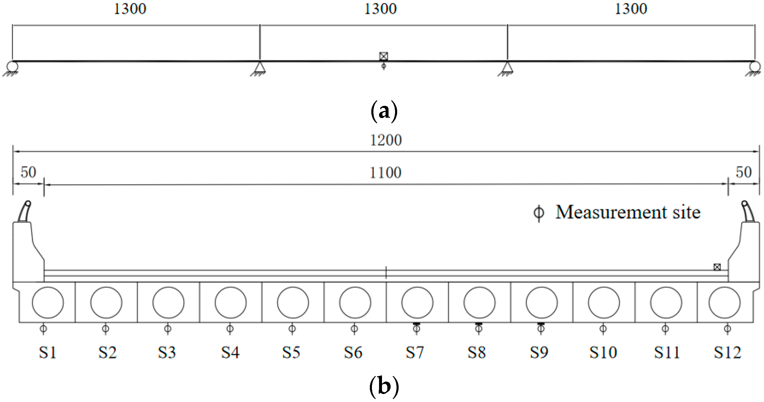
3.1. Case Description

This section presents a numerical application of the proposed method in a case bridge. Figure 2a,b illustrates the geometry of the case bridge, which has a superstructure consisting of three 13-m simply supported hollow slab spans, each with 12 hollow slabs, denoted as S1 to S12, respectively. The geometry of the cross-section is illustrated in Figure 2b. The substructure of the case bridge includes double-column piers and frame abutments, with simple oil felt pad bearings.

The bridge was reinforced with an FRP fiber plate, and loading tests were made before and after the reinforcement. The loading location and details of the loading vehicles are presented in Figure 3 and

Table 1. Axial distribution and weights of the loading vehicle.

Axial Weight (t)			Distance (cm)
Axe 1	Axe 2	Axe 3	A	B	C
6.24	12.24	11.88	445	140	185

, respectively. During the loading tests, data of mid-span deflections of each hollow slab were measured. The measured deflections were used to conduct the Bayesian inference of damage states based on the method proposed in this paper. Measurement points were placed at the mid-span section of the second span, and the locations of the measurement points within the cross-section are presented in Figure 3. Table 1 presents the distribution of axial weights for the loading vehicle. The total weight of the loading vehicle is 30.36 t, which is distributed on axes 1, 2, and 3, as illustrated by Table 1.

As presented in Figure 4, two sets of deflection were measured at the bottom of each slab before and after the reinforcement. These deflection measurements are used as the target D for the Bayesian inference formulated as Equation (5), so as to calibrate the damage states of the bridge.

3.2. Model Setup

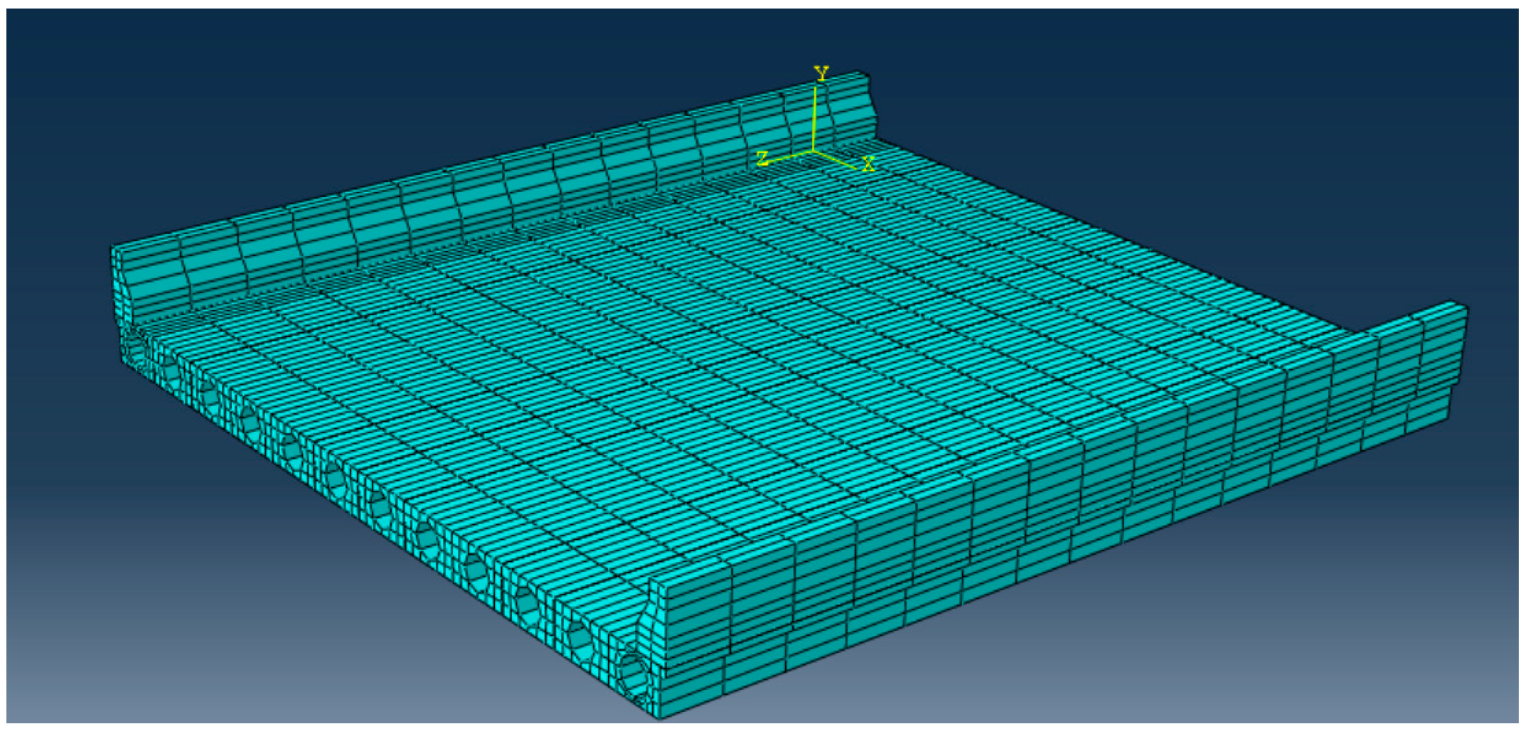
3.2.1. The FEM to Compute the Bridge Deflection

As presented in Figure 5, an FEM of the case bridge was established using ABAQUS. Based on the design documents, only span 2 was modeled considering the simply supported boundary condition. The damage state of span 2 is most correlated with the test data and is therefore specifically considered in the Bayesian inference for assessing structural conditions. The connections among the concrete slab bridge are fixed connections, which are simulated by the shared nodes between adjacent slabs in the FEM model.

As formulated in Equation (1), each of the 12 slabs is assigned with a damage indicator d_i (i = 1, 2, 3…12), which is spatially correlated and governed by the stochastic field generated by Equation (2). Following the KL transform described in Equation (2), the distribution modes of the stochastic fields, i.e., $\sqrt{{\lambda }_m}{f}_m(m=1,2\dots 12)$, are derived. Here, the autocorrelation function R in Equation (4) is determined as an exponential form:

$$R=\exp (-{\displaystyle \frac{\Delta x}{L}})$$

(16)

where ∆x denotes the distance between the centers of two slabs; L is the critical length of the autocorrelation function. In this paper, L is assumed to be the width of the slab. The weights of the distribution modes θ_i (i = 1, 2, 3…12) are subject to the Bayesian inference.

3.2.2. Kriging Surrogate of the FEM

A Kriging surrogate model of the FEM is constructed to improve the computational efficiency of the Bayesian inference. Following the LHC algorithm detailed in Section 2.3.2, 500 DOEs are selected in the parameter space of θ_i (i = 1, 2, 3…12). The deflection data at the measurement sites in Figure 6b are obtained as the output of the DOEs.

To derive the DOEs, a Python script was used to convert the model input θ into the stochastic field of damage states d and then use Equation (1) to modify the stiffness of each slab in the ABAQUS. The established FEMs are demonstrated in Figure 6.

3.2.3. Model Parameters for the MCMC Sampler

As detailed in Section 2.3, a Gauss transition kernel is used for the MCMC sampler, which can satisfy the detailed balance condition of the Markov chain. The standardized deviation of the transition kernel is determined as 0.01 for θ_i (i = 1, 2, 3…12). The start point of the Markov chain is chosen as the θ = 1, where 1 denotes a unity vector.

A total number of 50,000 samples are drawn along the Markov chain, in which the first 10% of samples (i.e., 5000 samples) are discarded to ensure that the samples can populate the important regions of the posterior distribution.

3.3. Results and Discussion

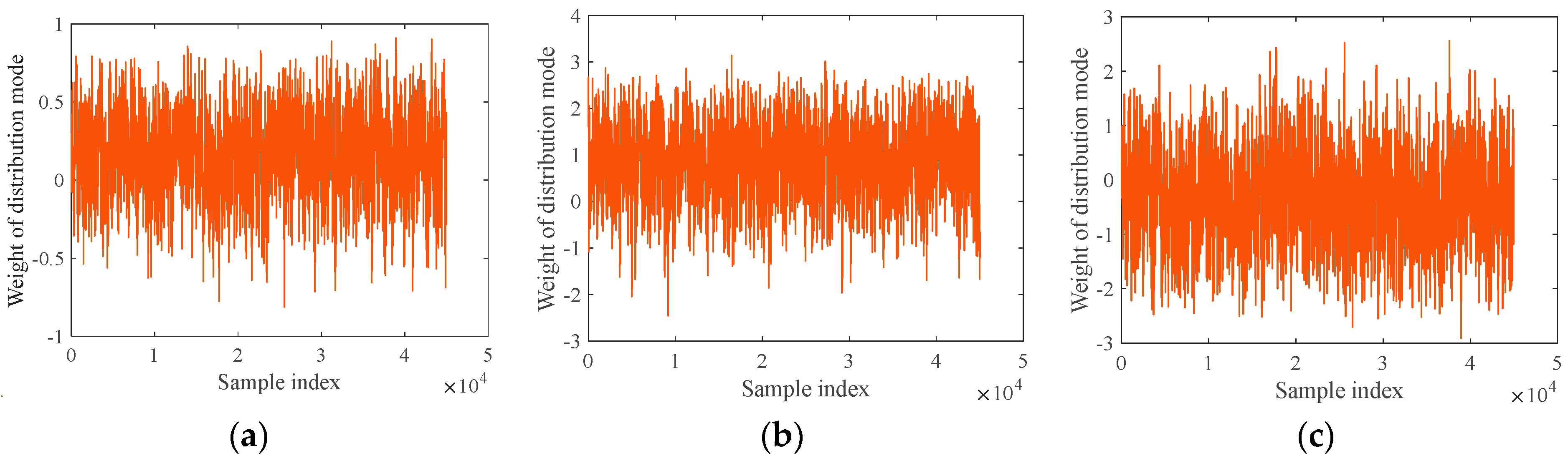
3.3.1. Inference Results of the Weights of Damage Distribution Modes

Figure 7 illustrates the evolution of the samples of the mean damage indicator d₀, as defined by Equation (2), along the Markov chain. It is indicated that both the damage indicator samples before and after the reinforcement are stable along the Markov chain, which justifies the convergence of the MCMC sampler and the validity of the drawn samples. Furthermore, the results suggest significantly lower values of d₀ after the update, which manifests the improvements in structural rigidity after the reinforcement.

Figure 8 presents the developments of the weights of the distribution modes along the Markov chain, denoted as for θ_i (i = 1, 2, 3…12), which suggests a relatively stable evolution of these weights along the Markov chain. The acceptance rate of these weights is 75.63%, which ensures the samples sufficiently explore the important regions of their joint posterior distribution, and the drawn samples can be used to approximate the statistics of the joint posterior distribution. In addition, the variances of the weights are different, which suggests the different contributions of the distribution modes in the reconstruction of the damage distribution. For example, the contribution of the first distribution mode is relatively insignificant, which is manifested by the smaller values of θ₁. On the other hand, as suggested by the larger values of θ₁₂, the contribution of the 12th distribution is significant.

Figure 9 presents the samples of θ_i (i = 1, 2, 3…12) drawn according to the deflection measured after the reinforcement of the case bridge. The samples are shown to feature stable evolution along the Markov chain, with an acceptance rate of 62.29%, which suggests that the samples can efficiently explore the posterior distribution of θ_i (i = 1, 2, 3…12) after the reinforcement.

Table 2. Statistics of θ before and after the reinforcement.

Variables		θ1	θ2	θ3	θ4	θ5	θ6	θ7	θ8	θ9	θ10	θ11	θ12
Before Reinforcement	Mean	−0.081	−0.091	0.035	0.055	−0.045	−0.067	−0.105	−0.089	−0.033	0.023	0.059	0.006
	Stdev	1.006	0.980	0.974	1.016	0.987	0.959	0.986	1.065	0.987	0.974	0.991	0.302
Before Reinforcement	Mean	0.184	−0.158	0.155	−0.119	−0.194	−0.169	−0.205	−0.417	−0.363	−0.365	0.873	0.167
	Stdev	0.960	0.963	0.954	0.979	0.973	0.953	0.951	0.937	0.949	0.820	0.755	0.258

presents a comparison between the mean and standardized deviation of θ before and after the reinforcement. Compared to the samples drawn before the reinforcement, the sample values of θ₁₂ are significantly smaller, which suggests the less significant contribution of the 12th distribution mode of damage distribution. This observation can be explained by the fact that the 12th distribution mode, as illustrated in Figure 9, is characterized by the high-frequency variation of damage distribution. After the reinforcement, the stiffness of the hollow slabs is improved comprehensively and the contribution of the high-frequency component becomes less significant.

3.3.2. Inference Results of the Damage States

Figure 10 illustrates the marginal posterior distributions of the damage indicators d_i (i = 1, 2, 3…12) for each slab of the bridge before the reinforcement, which is calculated based on the posterior distribution of the weight vector θ.

It is indicated that the damage indicators all approximately follow the Gauss distribution, with their mean values centered around the undamaged state (d = 1). Their averages and standardized deviations are used for further investigation of the damage states.

Figure 11 presents the marginal posterior distributions of the damage indicators of each hollow slab after the reinforcement of the case bridge. The marginal distributions all follow Gauss distributions, and the averages and standardized deviations of the distributions are used to characterize the distributions.

Figure 12 illustrates the averages and 95% confidence bounds (CBs) for the damage indicators before and after the reinforcement of the case bridge. The data indicate that the indicators increased significantly in all hollow slabs following the reinforcement, suggesting an improvement in structural rigidity. After the reinforcement, the 95% lower confidence bound of the structural rigidity indicator nearly overlaps with the undamaged state (d = 1), indicating that the reinforcement has effectively restored the structural rigidity to meet the design criterion.

Figure 13 and Figure 14 show the deflections calculated from the updated model parameters before and after reinforcement. The figures demonstrate the average deflection of the updated model and the 95% confidence bounds of the deflection. It can be observed that the average deflection of the updated model matches well with the measured deflection before and after reinforcement. The 95% deflection confidence bounds (the shadow area in Figure 13 and Figure 14) of the updated model effectively encompass almost all deflection measurements. This indicates that the updated model’s stiffness distribution closely matches the measured deflection values. In other words, the stiffness distribution obtained through the update represents the most likely stiffness distribution based on the measured deflection values, demonstrating an effective inversion result. Therefore, the conclusion that the structural stiffness improvement is valid and reliable.

4. Conclusions

In this paper, a Bayes inference frame was established to update the structural rigidity ratio of an aging hollow slab RC bridge based on the deflection measurement of the bridge. Major conclusions are listed as follows:

• The structural rigidity ratio of the aging RC bridge is modeled as a stochastic field along the hollow RC slabs using the KL transform, and the weights of the distribution modes of structural rigidity were used as the model parameters subject to Bayes inference, which can capture the spatial correlation and variation of the structural rigidity.
• The structural rigidity ratio of the aging RC bridge was updated based on the Bayesian inference using the deflection measured during a static loading test. The Bayesian inference leverages the information from a FEM that computes the deflection of the bridge, and a Kriging surrogate model of the FEM was constructed to improve the computation efficiency. The posterior distribution of the structural rigidity ratio was derived by an MCMC sampler, and the drawn samples were used to approximate the statistics of the posterior distributions.
• The proposed method was applied on a RC case bridge with hollow slabs, based on two sets of deflection measurements before and after the reinforcement of the case bridge. The Bayes updates using the deflection measurements suggest higher structural rigidity ratios among the hollow slabs after the reinforcement, which quantitatively justifies the effectiveness of the reinforcement. The deflection calculated by the updated models can well match deflection measurements, with the 95% CBs of deflection including most of the measurements, which justifies the validity and robustness of the proposed method.

The proposed method can be used to update the status of concrete slab bridges and assess the efficiency of reinforcement. To ensure the reliability of the algorithm, it is necessary to use structural monitoring data from different times to interpolate structural information and track the time dependency of structural states. Additionally, it is important to further use heterogeneous data beyond deflection for the Bayesian inference, which can be achieved by establishing a framework capable of processing information from various sources to enhance the reliability of the Bayesian inference.

References

1. Ministry of Transport of the People’s Republic of China. Annual Report on China’s Roadway Network; Ministry of Transport of the People’s Republic of China: Beijing, China, 2023.
2. Pimentel, M.; Garcez, C. Challenges in the maintenance of concrete bridges. J. Civ. Eng. Manag. 2018, 24, 125–136. [Google Scholar]
3. Bian, L.; Wang, G.; Liu, P. Reliability analysis for multi-component systems with interdependent competing failure processes. Appl. Math. Model. 2021, 90, 543–556. [Google Scholar] [CrossRef]
4. Yang, Y.; Wang, H.; Sangwongwanich, A. Design for reliability of power electronic systems. Power Electron. 2018, 12, 130–141. [Google Scholar] [CrossRef]
5. Alaswad, S.; Xiang, Y. A review on condition-based maintenance optimization models for stochastically deteriorating systems. Reliab. Eng. Syst. Saf. 2017, 159, 399–414. [Google Scholar] [CrossRef]
6. Zhai, W.; Han, Z.; Chen, Z.; Ling, L.; Zhu, S. Train–track–bridge dynamic interaction: A state-of-the-art review. Veh. Syst. Dyn. 2019, 57, 1139–1176. [Google Scholar] [CrossRef]
7. Sun, L.; Shang, Z.; Xia, Y.; Bhowmick, S. Review of bridge structural health monitoring aided by big data and artificial intelligence: From condition assessment to damage detection. J. Struct. Eng. 2020, 146, 04020144. [Google Scholar] [CrossRef]
8. Wang, L.; Wang, X.; Su, H.; Lin, G. Reliability estimation of fatigue crack growth prediction via limited measured data. Int. J. Mech. Sci. 2017, 131–132, 1065–1078. [Google Scholar] [CrossRef]
9. Tidriri, K.; Chatti, N.; Verron, S.; Tiplica, T. Bridging data-driven and model-based approaches for process fault diagnosis and health monitoring: A review of researches and future challenges. Annu. Rev. Control 2016, 42, 63–81. [Google Scholar] [CrossRef]
10. Melchers, R.E.; Beck, A.T. Structural reliability analysis and prediction. J. Struct. Saf. 2018, 9, 210–221. [Google Scholar] [CrossRef]
11. Li, W.; Liu, Y. A new method for the fatigue life prediction of bridge structures. J. Bridge Eng. 2018, 23, 04518013. [Google Scholar] [CrossRef]
12. Guan, H.; Zhong, J.; Bai, L. Reliability assessment of large-span bridge structures under multi-hazard conditions. Struct. Infrastruct. Eng. 2020, 16, 128–143. [Google Scholar]
13. Gunawan, F.E. A new damage indicator in time and frequency domains for structural health monitoring: The case of beam with a breathing crack. Int. J. Innov. Comput. Inf. Control 2020, 16, 507–519. [Google Scholar]
14. Boscato, G.; Fragonara, L.Z.; Cecchi, A.; Reccia, E. Structural health monitoring through vibration-based approaches. Shock Vib. 2019, 2019, 2380616. [Google Scholar] [CrossRef]
15. Peng, X.; Yang, Q.; Qin, F.; Sun, B. Structural Damage Detection Based on Static and Dynamic Flexibility: A Review and Comparative Study. Coatings 2023, 14, 31. [Google Scholar] [CrossRef]
16. Wang, F.; Li, R.; Xiao, Y.; Deng, Q.; Li, X.; Song, X. A strain modal flexibility method to multiple slight damage localization combined with a data fusion technique. Measurement 2021, 178, 109442. [Google Scholar] [CrossRef]
17. Gharehbaghi, V.R.; Noroozinejad Farsangi, E. A critical review on structural health monitoring: Definitions, methods, and perspectives. Arch. Comput. Methods Eng. 2022, 29, 1687–1715. [Google Scholar] [CrossRef]
18. Ali, J.; Bandyopadhyay, D. Condition monitoring of structures using limited noisy data modal slope and curvature of mode shapes. Int. J. Struct. Integr. 2020, 11, 309–321. [Google Scholar] [CrossRef]
19. Zhang, J.; Li, A.; Wang, T. Monitoring of deflections in bridges: A review. J. Bridge Eng. 2013, 18, 321–330. [Google Scholar] [CrossRef]
20. Brownjohn, J.M.W. Structural health monitoring of civil infrastructure. Philos. Trans. R. Soc. A Math. Phys. Eng. Sci. 2007, 365, 589–622. [Google Scholar] [CrossRef]
21. Cross, E.J.; Worden, K.; Farrar, C.R. Structural health monitoring for civil infrastructure. Annu. Rev. Civil Eng. 2013, 5, 429–462. [Google Scholar] [CrossRef]
22. Peeters, B.; De Roeck, G. One-year monitoring of the Z24-Bridge: Environmental effects versus damage events. Earthquake Eng. Struct. Dyn. 2001, 30, 149–171. [Google Scholar] [CrossRef]
23. Hedegaard, C.M.; Schmidt, J.W.; Ravn, J.D. Structural health monitoring of the Great Belt Bridge. Bridge Struct. 2015, 11, 124–133. [Google Scholar]
24. Yan, A.M.; Kerschen, G.; De Boe, P.; Golinval, J.C. Structural damage diagnosis under varying environmental conditions—Part I: A linear analysis. Mech. Syst. Signal Process. 2005, 19, 847–864. [Google Scholar] [CrossRef]
25. Sanayei, M.; Samaan, M.; Morgan, R.Q.; Brenner, B.R. Damage localization and finite-element model updating using multi-response NDT data. J. Bridge Eng. 2001, 6, 238–247. [Google Scholar] [CrossRef]
26. Sanayei, M.; Samaan, M.; Morgan, R.Q.; Brenner, B.R. Analysis and identification of structural stiffness from displacement measurements. J. Struct. Eng. 1997, 123, 1148–1155. [Google Scholar]
27. Sanayei, M.; Douglas, B.S.; Burke, J.C. Structural model updating using experimental static measurements. J. Struct. Eng. 1991, 117, 1993–2008. [Google Scholar] [CrossRef]
28. Sanayei, M.; White, T.L.; Charnis, D.J. Stiffness calibration of truss model for supporting structure of large radio antennas. J. Aerosp. Eng. 1999, 12, 24–34. [Google Scholar]
29. Sanayei, M.; Bell, E.S. Structural model updating using deflection data from static tests. J. Bridge Eng. 2004, 9, 391–398. [Google Scholar] [CrossRef]
30. Banan, M.R.; Hjelmstad, K.D. Parameter estimation of structures from static response. I. Computational aspects. J. Struct. Eng. 1994, 120, 3243–3258. [Google Scholar] [CrossRef]
31. Banan, M.R.; Hjelmstad, K.D. Parameter estimation of structures from static response. II. Numerical simulation studies. J. Struct. Eng. 1994, 120, 3259–3283. [Google Scholar] [CrossRef]
32. Beck, J.L.; Katafygiotis, L.S. Updating models and their uncertainties. I: Bayesian statistical framework. J. Eng. Mech. 1998, 124, 455–461. [Google Scholar] [CrossRef]
33. Beck, J.L.; Katafygiotis, L.S. Updating models and their uncertainties. II: Model identifiability. J. Eng. Mech. 1998, 124, 463–467. [Google Scholar] [CrossRef]
34. Nettis, A.; Nettis, A.; Ruggieri, S.; Uva, G. Corrosion-induced fragility of existing prestressed concrete girder bridges under traffic loads. Eng. Struct. 2024, 314, 118302. [Google Scholar] [CrossRef]
35. Zhang, Q.; Zhang, Q.; Karbhari, V.M. Applications of the Karhunen–Loève transform for health monitoring of bridge systems. Smart Mater. Struct. 2006, 15, 131–139. [Google Scholar] [CrossRef]
36. Han, B.; Xiang, T.Y.; Xie, H.B. A Bayesian inference framework for predicting the long-term deflection of concrete structures caused by creep and shrinkage. Eng. Struct. 2017, 142, 46–55. [Google Scholar] [CrossRef]
37. Sun, L.; Mahadevan, S. Reliability assessment of structural systems using Kriging-based models. Struct. Saf. 2007, 29, 97–112. [Google Scholar]
38. Santner, T.; Williams, B.; Notz, W. The Design and Analysis of Computer Experiments; Springer: New York, NY, USA, 2003. [Google Scholar]
39. Iman, R.L.; Helton, J.C.; Campbell, J.E. An Approach to Sensitivity Analysis of Computer Models: Part I—Introduction, Input Variable Selection and Preliminary Variable Assessment. J. Qual. Technol. 1981, 13, 174–183. [Google Scholar] [CrossRef]
40. Beck, J.L.; Au, S.K. Bayesian updating of structural models and reliability using Markov chain Monte Carlo simulation. J. Eng. Mech. 2002, 128, 380–391. [Google Scholar] [CrossRef]
41. Chib, S.; Greenberg, E. Understanding the Metropolis-Hastings Algorithm. Am. Stat. 1995, 49, 327–335. [Google Scholar] [CrossRef]
Figure 1. Illustration of the damage indicator for the RC hollow slab bridge.
Buildings 14 02920 g001
Figure 2. Geometry of the case bridge (in cm). (a) Longitudinal geometry of the case bridge; (b) cross-section geometry of the case bridge.
Buildings 14 02920 g002
Figure 3. Geometry of the case bridge (in cm). (a) Longitudinal view of the loading condition; (b) cross-section geometry of the loading condition.
Buildings 14 02920 g003
Figure 4. Deflection measurements before and after the reinforcement.
Buildings 14 02920 g004
Figure 5. FEM of the case bridge.
Buildings 14 02920 g005
Figure 6. DOEs for the Kriging surrogate. (a) Model 1; (b) Model 10; (c) Model 131; (d) Model 207; (e) Model 237; (f) Model 309; (g) Model 345; (h) Model 422; (i) Model 481.
Buildings 14 02920 g006
Figure 7. Evolution of the mean damage indicator d0 along the Markov chain.
Buildings 14 02920 g007
Figure 8. Developments of the weights of the distribution modes along the Markov chain (before update). (a) θ1; (b) θ2; (c) θ3; (d) θ4; (e) θ5; (f) θ6; (g) θ7; (h) θ8; (i) θ9; (j) θ10; (k) θ11; (l) θ12.
Buildings 14 02920 g008aBuildings 14 02920 g008b
Figure 9. Developments of the weights of the distribution modes along the Markov chain (after update). (a) θ1; (b) θ2; (c) θ3; (d) θ4; (e) θ5; (f) θ6; (g) θ7; (h) θ8; (i) θ9; (j) θ10; (k) θ11; (l) θ12.
Buildings 14 02920 g009aBuildings 14 02920 g009b
Figure 10. Marginal posterior distributions of the damage indicators (before update). (a) d1; (b) d2; (c) d3; (d) d4; (e) d5; (f) d6; (g) d7; (h) d8; (i) d9; (j) d10; (k) d11; (l) d12.
Buildings 14 02920 g010
Figure 11. Marginal posterior distributions of the damage indicators (after update). (a) d1; (b) d2; (c) d3; (d) d4; (e) d5; (f) d6; (g) d7; (h) d8; (i) d9; (j) d10; (k) d11; (l) d12.
Buildings 14 02920 g011
Figure 12. The averages and 95% confidence bounds (CBs) for the damage indicators before and after the reinforcement.
Buildings 14 02920 g012
Figure 13. Validation of the updated model parameters before reinforcement.
Buildings 14 02920 g013
Figure 14. Validation of the updated model parameters after reinforcement.
Buildings 14 02920 g014