Passive Control Measures of Wind Flow around Tall Buildings

Abstract

The growth and diversification of tall buildings demands higher performance standards that encompass serviceability and resilience. In this respect, the control of air flow around tall buildings poses challenges to minimising the energy that could induce large vibrations or forces. The present investigation scrutinises the flow around a tall structure with variations on its surface roughness by adding balconies to the facade, as a form of passive control of the flow loads. This is conducted through flow simulations across optimised computational arrays that capture 3D effects. To illustrate the applicability of the proposed approach, two types of facades rotated $0^{\circ }$, ${90}^{\circ }$ and ${180}^{\circ }$ are considered while focusing on pressure and vorticity fields. It was found that the presence of balconies produces zig-zag patterns on the face where they are located, whereas balconies on the front facade reduce drag with respect to the smooth case. Furthermore, buildings with balconies on their lateral faces experience some increase in drag force and the improvement of the aerodynamics around the lateral pedestrian zones. No qualitative variations between triangular and rectangular balconies were found, excepting some changes in pressure magnitude on the rear side induced by balconies placed on the front and rear facades. Through the comparison of results, it was confirmed that the findings align with previous studies undertaken for medium and low-rise buildings. This reinforces the proposal of using such passive control measures to improve the aerodynamic performance of tall buildings. The study enables the quantification of flow configurations and forces on the building’s faces. Some of the proposed passive control measures effectively mitigate pressure levels while causing large local disturbs on pressure and vorticity that should be attended to by designers of this type of facades.

1. Introduction

1.1. Passive Control Measures

Civil Engineering Institutions are developing a new framework for wind resistant design that identifies definite performance objectives [1]. The American Society of Civil Engineers (ASCE) and International Building Code (IBC) [2] have established performance objectives within their own frameworks addressing Occupant Comfort, Operational, and Continuous Occupancy with Limited Interruption. According to this, any new design will require the initial categorisation of risk associated with the target performance objective, to then observe the acceptance criteria for structural and non-structural components. This deviates from the traditional performance-based design (PBD) philosophies oriented to structural components that eventually undergo inelastic performance. The PDB for wind actions [1] addresses more thoroughly potential damage on the building envelope and non-structural components yet allows specific elements of the main structural system to withstand plastic deformations under extreme events.

The search for passive control mechanisms to mitigate flow disturbances and structural vibrations spans various decades. It was stated since pioneering studies like that performed by [3] for an experiment representing a 120 m height square building with equispaced balconies of 2 m and 4 m wide (with and without vertical walls) attached to one wall of the building; they concluded from experimental data that the presence of balconies in the facade reduce slightly the pressure coefficient values on the building surface, while the effect increases for balconies with walls and their effect becomes more significant at the lower part of the building for all azimuths. Similar results were found in [4], using wind tunnel data from models that simulate a 75 m high square building with balconies in all walls (with and without mullion), ranging 0.63–2.5 m wide with constant separation that simulated 26 floors; they concluded that wind pressures were remarkably affected by the surface roughness, particularly near the leading edge of the side wall on which local severe peak pressures decrease when increasing the roughness. In the same line, refs. [5,6] studied the aerodynamic forces on high-rise buildings with various facade appurtenances, by considering a prototype that simulates a 150 m high building with horizontal plates above half the height of the building, resembling balconies with various vertical separations. The first study found that the locations of the largest positive peak pressures can be strongly affected by the vertical arrangement of the horizontal plates, whereas the largest negative peak pressure on the higher leading corner is significantly reduced with respect to the smooth surface case. Regarding the second one, they observed a “zig-zag” pattern in both along-wind and cross-wind layer forces which are closely related to the vertical separation of adjacent appurtenances, specifically when the separation is more than 4% (6 m in real scale).

On the other hand, passive measures also include passive bracing made of low yield steel that according to [7] could reduce the base shear by up to 20% for moderate external forces Other methods propose the use of screen meshing to modify the topology of building facades [8] which are meant to improve flow reattachment and decreases the possibility of damage due to pressure fluctuations. However, the referred studies indicate that the applicability of screen meshing is mildly effective for low-rise buildings. The passive control system on the building envelope was later replaced with double-skin facades intended to mitigate wind-induced vibrations. Experimental studies discussed in [9] show that although the double-skin facades did not seem to change the along-wind response, some improvements could be reported for crosswind vibrations of facades with openings. The solution does not seem optimal, since the results of the same study highlight that facades with openings tend to increase the forces in the along-wind direction of the model tested. A similar solution based on a smart morphing facade system was presented in [10]. This system consists of ducts (openings) distributed across the external layer equipped with fan-like parts that rotate with the wind flow. As the movable parts rotate the porosity of the surface changes, which enables a force decrease of around 20–30%, depending on the wind direction, although one should note that such a level of improvement corresponds to mechanisms covering the entire surface of facades which leaves little space for windows and other services. Further passive control measures have been explored involving geometrical modifications. Examples of these include variations of the building’s cross-section such as chamfered, rounded, triangle, recessed, or slotted corners; as well as shape variations along the building height such as tapering, twisting, setbacks, openings, and spoilers, see [11]. From amongst these alternatives, the most popular ones are double-facade systems and changes in building geometry, particularly the latter which according to [11] enables load reductions between 30% and 60%.

1.2. CFD in Buildings Design

Computational Fluid Dynamics (CFD) stands amongst the most effective methods to determine wind-structure interactions. Ref. [12] broadly discusses the requirements that CFD simulations should fulfill to satisfactorily reproduce wind tunnel measurements. They cover the simulation of fluid-structure interaction based on the Lattice Boltzmann and Smoothed Particles. Likewise, ref. [13] presents a complete review of the most important technical aspects to be considered in CFD studies on high-rise buildings. For example, the atmospheric boundary layer where the mean wind speed develops should describe a logarithmic variation with height taking as reference the mean wind speed recorded at 10 m above the ground level, while complemented with variations of the turbulence intensity along a vertical coordinate, as used in the simulations presented by [14]. CFD simulations of this kind initialise the wind with at least 2–5 Flow Through Domain (FTD) units, to then quantify the sampling interval in terms of either (a) peak pressures on the building (references therein estimate around 5–15 peaks), or (b) time in full scale (commonly suggested 10 min).

Furthermore, turbulence frameworks ought to be applied in realistic models, like locating Large Eddy Simulations (LES) over Reynolds-averaged Navier–Stokes (RANS) and hybrid methods [13]. These numerical schemes highly recommend at least second-order finite difference schemes for time discretisation, while Total Variation Diminishing (TVD), Upwind Schemes, Central Difference Scheme (CDS), or bounded version for spatial discretisation. They highlight the importance of implementing a high mesh resolution near walls to be determined according to the shortest side of the building and with prism layers stretching with a maximum ratio of 1.05, especially when surface pressures in those regions are of interest. The authors emphasize that these are suggested values, such that an appropriate numerical simulation could combine these according to the project needs and the computational resources at hand.

As stated above, past research have simulated wind-structure interactions by modifying building envelopes with stepped [15], octagonal [16] and atypically shaped [17] faces, as well as plan-shaped prototypes [18], that have shown significant variations of the pressure coefficient ($Cp$) with the building height, the wind incidence angle, and both the incidence angle and the rounding of corners. For example, ref. [19] suggested that wrinkled surfaces such as balconies, should be taken into account when performing CFD, since these can induce flow separation and recirculation, leading to large disturbances of the wind pressure distribution on facades. They supported this idea by simulating 3D steady RANS for medium-rise buildings with and without balconies, for which they found results in good agreement with wind-tunnel measurements taken at the perpendicular flow direction with respect to the area exposed, although larger discrepancies (underestimations) for other yaw angles. More recently, ref. [20] performed a similar study comparing RANS and LES results for an isolated high-rise building exposed to varying the wind direction. They concluded that RANS generally underestimates ventilation airflow rates and wind speed ratios, which would lead to building designs with high levels of nuisance for end users. Finally, ref. [21] completed an exhaustive study on the implementation of balconies in numerical models; those being characterised by protruding depth and density, the presence of parapets and partition walls. From LES, they found a configuration of partition walls that can reduce by up to 68.0% the area-averaged wind speed across balcony spaces.

1.3. Work’s Objective

In the context stated above, the most of CFD studies investigating the impact of building balconies have used steady RANS, as stated in [20]. A few investigations based on LES and SAS (Scale Adaptative Simulation) have focused on medium to low-rise buildings (5–22 stories), while adding different types of rectangular balconies on one wall, and rotating the building from $0^{\circ }$ to ${90}^{\circ }$. Examples of those works are [19,22,23,24,25,26,27,28,29]. They have investigated mixed parameters such as average speed around the envelope, pressure coefficients, concentration of pollutants, and convective heat transfer. This highlights the novelty of the present study, which models a tall building of 200 m height with triangular and rectangular balconies on the front, side, and rear facades by LES while limiting the result to pressure coefficients and vorticity level. Besides the contribution to CFD studies, this work contrasts with previous research such as [4,5,6], which conducted experimental testing on buildings with rough facades, however, using different building size, façade system, or roughness configuration, to the ones presented in this work. The investigation thus attempts to enhance the knowledge and understanding of the aerodynamic performance of tall buildings with facades fully covering the front, side, and rear walls, providing further insight on pressure distributions obtained under strong winds, which could enable to progress PBD code initiatives for wind resisting design.

The paper is structured as follows: Section 2 provides the numerical method. Section 3 shows the technical aspects of the study and the validation of the computational model. Section 4 describes the numerical results. Section 5 discusses the findings, while Section 6 provides some concluding remarks.

2. Method

The CFD simulations were carried out by using OpenFOAM (version v2012, december 2020, released by OpenCFD Ltd.—ESI Group, mainly located in Bracknell, UK) [30], which is a free, open source software that solves the Navier–Stokes equations by the finite volume method. OpenFOAM was selected mainly because it is a highly functional and freely available open source CFD software. It has a large user base in science and engineering, including the reproduction of flow around different types of buildings with satisfactory results, see [31,32,33] and references therein. Therefore, simulations could be easily reproduced or extended in case high cost license software like ANSYS Fluent (version 2024R1, January 2024), COMSOL (version 6.2, november 2023), FLOW-3D (version 2023R2, December 2023), etc., are not available.

Under a Delayed Detached Eddy Simulations (DDES) construction, the Spalart–Allmaras (SA) model [34,35] was selected as the closure of the system, which is a one equation model based on a modified turbulence viscosity $\tilde{\nu }$, and includes a destruction term depending on the distance to the nearest wall as follows:

$$\frac{D}{Dt}\left(\rho \tilde{\nu }\right)=\nabla ·\left(\rho D_{\tilde{\nu }}\tilde{\nu }\right)+\frac{g_{b2}}{{\sigma }_{{\nu }_t}}\rho {|\nabla \tilde{\nu }|}^2+g_{b1}\rho \tilde{\zeta }\tilde{\nu }-g_{w1}{f}_w\rho {\left(\frac{\tilde{\nu }}{\tilde{d}}\right)}^2+{\zeta }_{\tilde{\nu }}.$$

(1)

where $\rho$ is the density of the fluid, $\zeta$ is the shear stress, and the turbulent viscosity (${\nu }_t$) is recovered from $\tilde{\nu }$ by means of a correction involving viscosity ($\nu$):

$${\nu }_t=\tilde{\nu }\frac{{\chi }^3}{{\chi }^3+g_{v1}^3},\chi =\frac{\tilde{\nu }}{\nu },$$

(2)

where $g_{v1}$ is a constant. In turn, $\tilde{d}$ is the length scale defined by

$$\tilde{d}=\max \left[L_{RAS}-f_d,\max (L_{RAS}-L_{LES},0)\right],$$

(3)

so that, Equation (3) varies the length scale in Equation (1) according to the proximity to the closest solid wall. According to this, the length scale is estimated (i) with a full RAS model ($L_{RAS}$) when it is far from the wall, $L_{RAS}=\lambda$, with $\lambda \equiv$ the distance from the analysed cell to the closest solid wall; (ii) with a full LES model ($L_{LES}$) when it is sensibly close, $L_{LES}=\psi g_{DES}\Delta$, with the MIN function $\psi \equiv \psi \left({\sigma }_{{\nu }_t}\right)$ as a low Reynolds number correction function, and $g_{DES}\Delta$ as a length proportional to the local grid spacing $\Delta =\max ({\Delta }_x,{\Delta }_y,{\Delta }_z)$, where $g_{DES}$ is a constant; (iii) and with a soften transition between scales by means of the delay function

$$f_d=1-\tanh \left[{\left(g_{d1}{\lambda }_d\right)}^{g_{d2}}\right],$$

(4)

where ${\lambda }_d\equiv {\lambda }_d(\mathbf{U},\nu ,\lambda )$ is a MIN function depending on the velocity vector of the fluid $\mathbf{U}=(U_x,U_y,U_z)$, its viscosity $\nu$ and the distance $\lambda$. This construction was fully implemented in a cube-root volume formulation by the function cubeRootVol. The parameters $f_w$, $g_{b1}$, $g_{b2}$, $g_{d1}$, $g_{d2}$, $g_{v1}$, $g_{w1}$, $g_{DES}$, ${\sigma }_{{\nu }_t}$ and functions $\psi$, ${\lambda }_d$, and the rest of the implicit parameters of the model were set to default values [36,37].

The methods and criteria provided by [13] were implemented to complete the discretisation of the flow equations and produce an algebraic system. Namely, a conditionally stable second-order implicit-backward was selected for the time scheme, Gauss linear for gradient schemes, Gauss linear limited for divergence and Laplacian schemes, and linear interpolation to transform the cell-centre quantities to face centres. Following, the Pressure Implicit with Splitting of Operators (PISO) algorithm was implemented to solve those equations, by considering a fully implicit formulation for pressure (coupled with velocity) with three corrections at each iteration [38]. The established solver methods were as follows: a generalised geometric-algebraic multi-grid for pressure, with the Gauss–Seidel method as a smoother, and a preconditioned pipelined conjugate residuals solver to override solution tolerance for the final pressure; in turn, a symmetric Gauss–Seidel solver for the rest of the variables.

3. Case Study

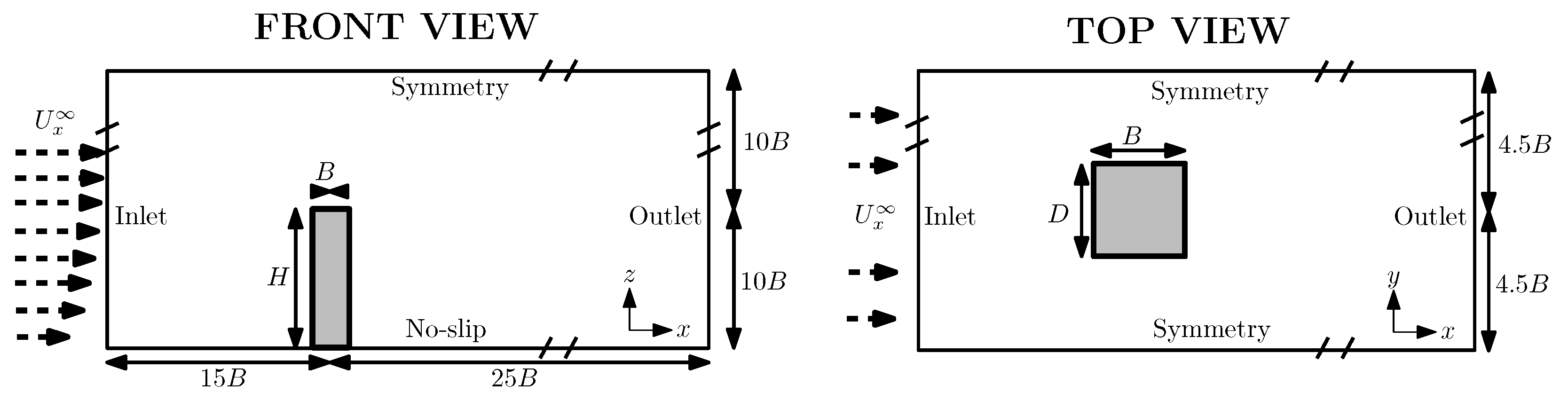
3.1. Meshing Details and Boundary Conditions

The building model is 20 m length (B), 20 m width (D), and 200 m height (H), generated within a computational environment, which according to the CTBUH Height Criteria classifies as tall-structure, as it lies in a suburb where is distinctly taller than the norm. Additionally to the smooth case, six non-smooth cases with structured facades were proposed by having balconies of triangular and rectangular shape. These balconies distribute across three building sides whose label and azimuth with respect to the wind direction are as follows: front ($0^{\circ }$), lateral (${90}^{\circ }$), and rear (${180}^{\circ }$). In detail, the roughness facade for such structures is modelled with 40 (triangular or rectangular) horizontal prisms equispatially distributed along a face of the building. The contour of each balcony fits half a (square or equilateral triangle) prism, whose base circumscribes about a circle of radius $\frac{B}{10}$, as illustrated in Figure 1 both for the (a) triangular and (b) rectangular balconies located at the front side.

Figure 2 shows the computational array in which the buildings are tested. The origin of the Cartesian coordinate system $(x,y,z)=(0,0,0)$m coincides with the geometric centre of the building’s base. Three zones with different types of grid and refinement levels (l) constitute the entire mesh, as seen in Figure 3a,b. Each level l approximates the cell size c by $c=\frac{B}{2^{l+1}}$. The finest grid (Zone A) is non-structured to fit the shape of the target geometry with $l=5$. In contrast, Zone B contains five levels of refinement which decrease with the distance from the building, spanning from level $l=5$ to $l=1$ as follows: $l=5$ covers up to a distance of $\frac{B}{20}$, $l=4$ up to $\frac{B}{5}$, $l=3$ up to $\frac{B}{2}$, $l=2$ up to $2B$, and $l=1$ up to $5B$. Finally, Zone C covers the rest of the array with level $l=0$. Furthermore, a transition of three cells between levels was established to obtain a smooth refinement. Zones A and B were constructed via the tool SnappyHexMesh, while Zone C via the tool blockMesh of OpenFOAM.

Table 1. Number of cells of each building case.

Geometry	Cells
Smooth	1,218,372
R0	1,281,564
R90	1,281,298
R180	1,281,501
T0	1,290,212
T90	1,289,638
T180	1,290,163

shows the number of cells forming the mesh of each building’s defined geometry. Each geometry is labelled according to the type of balcony (R ≡ rectangular, T ≡ triangular) and the azimuth (relative to the wind direction) of any vector normal to the facade holding the balconies, i.e., ($0\equiv$ front, $90\equiv$ lateral, $180\equiv$ rear). Each of the non-smooth geometries increases the number of cells by about 6% with respect to the smooth case.

To simulate the wind, log-law type ground-normal inflow boundary conditions were set for the stream-wise velocity ($U_x^{\infty }$) and turbulent kinetic energy (k) for the flow by using the class atmBoundaryLayer [39]. The corresponding equations are as follows:

$$U_x^{\infty }=\frac{U^{\ast }}{\kappa }\ln \left(\frac{z-d+z_0}{z_0}\right),$$

(5)

and

$$k=\frac{{\left(U^{\ast }\right)}^2}{\sqrt{{\beta }_m}}\sqrt{{\beta }_1\ln \left(\frac{z-d+z_0}{z_0}\right)+{\beta }_2},$$

(6)

where $\kappa$ is the von Kármán constant, $z_0$ is the aerodynamic roughness length (in m), d is the ground-normal displacement height (in m), ${\beta }_m$ is an empirical model constant, ${\beta }_1$ and ${\beta }_2$ are curve-fitting coefficient, and $U^{\ast }$ is the friction velocity that is calculated by

$$U^{\ast }=\frac{U_x^{ref}\kappa }{\ln \left(\frac{z^{ref}+z_0}{z_0}\right)},$$

(7)

where $U_x^{ref}$ is a reference mean streamwise wind speed at a reference height $z^{ref}$. The values of inflow parameters used for the simulations are shown in

Table 2. Parameters defining the inflow according to Equations (5)–(7).

Parameter	Value
$U_x^{ref}$	20 m/s
$z^{ref}$	10 m
$\kappa$	0.4 (dimensionless)
$z_0$	0.03 m
d	0.03 m
${\sigma }_m$	0.01 (dimensionless)
${\sigma }_1$	−0.05 (dimensionless)
${\sigma }_2$	1 (dimensionless)

, while the resulting streamwise velocity $U_x^{ref}$, and turbulence intensity I (estimated by $k=\frac{3}{2}{\left(UI\right)}^2$) profiles are shown in Figure 4. It follows that by taking B as the characteristic length, $U_x^{\infty }$ as the characteristic velocity profile, and considering standard air conditions, the resulting Reynolds numbers (Re) of the simulation becomes Re = $1.59\times {10}^7$ at $z=1$ m and Re = $4.01\times {10}^7$ at the top of the building ($z=200$ m).

The symmetry boundary was applied at the top, front and back limits of the array, while the no-slip boundary condition was at the bottom limit and at the buildings surface. In turn, Robin boundary condition was applied at the outlet by means of the class inletOutlet.

3.2. Modelling Validation

A preliminary study to achieve spatial convergence was undertaken. Four meshes with different refinement levels were tested by measuring drag, lateral forces, and pressure around the smooth building; meshes were labelled as M0, M1, M2, and M3. M2 is as described in Section 3.1, whereas M0 follows M2 but restricts the maximum refinement level to $l=3$, hence $l=4$ and $l=5$ in M2 become $l=3$ in M0. M1 introduces further changes with regards to M2 as it restricts cells within a distance of $\frac{B}{20}$ from the building to level $l=4$, while adjacent cells up to a distance of $\frac{B}{5}$ are restricted to level $l=3$. Finally, M3 follows M2 almost entirely but adds extra refinement at the edges of the building to reach up to level $l=7$.

Table 3. Temporal statistics for the results of drag and lift time series obtained from five combinations of mesh and simulated time.

Mesh	Cells	Simulated Time	${\mathit{Cd}}_{\mathit{avg}}$	${\mathit{Cd}}_{\mathit{rms}}$	${\mathit{Cl}}_{\mathit{avg}}$	${\mathit{Cl}}_{\mathit{rms}}$
M0	340,684	3 min	1.31	0.09	−0.04	0.45
M1	480,103	3 min	1.28	0.07	−0.01	0.34
M2	1,218,372	3 min	1.29	0.07	0.02	0.31
M2	1,218,372	10 min	1.30	0.07	0.00	0.34
M3	1,812,462	3 min	1.30	0.06	0.01	0.36

summarises the results of those simulations. It is seen in this table that convergence occurs across average ${(\ast )}_{avg}$ and RMS ${(\ast )}_{RMS}$ for both drag $Cd$ and lift $Cl$ coefficients, with the increase in the refinement level for 3 min simulations. Indeed, the intermediate and finest meshes M1-M3 provide similar results while the coarsest mesh M0 differs from them by duplicating the average lateral effect $C{l}_{avg}$ and increasing the fluctuating effect $C{l}_{RMS}$ one and a half times, respecting to M2. This observation is supported by the results shown in Figure 5a,b, where it could be observed that M0 is the mesh showing somewhat different average $C{p}_{avg}$ and RMS $C{p}_{RMS}$ of pressure coefficient around the building at $z=\frac{2}{3}H$, particularly at the lateral side. Nevertheless M1 is able to produce similar force patterns than higher refinement meshes, M2 is taken forward to determine the aerodynamic performance of the building with higher precision. This takes into account that for non-smooth buildings and in accordance with Section 3.1, the upper balcony sides are reproduced with about 2–3 cells by M1 and 5–6 cells by M2, which approximates previous mesh arrays in the literature with 6 cells [20,21], and 8 cells [19].

Furthermore, an additional 10 min test with mesh M2 was carried out to validate the duration of the simulation, see Figure 6, following the Thordal et al.’s suggestion [13] of capturing the effects of flow during at least 10 peaks (not mandatory, as mentioned in references therein). Even though only one peak per minute is captured, the sampling interval was set to a duration of 3 min since no significant deviations were found with the 10 min simulation, as also seen in Table 3 and Figure 5.

Following [13], the preliminary simulations shown in Figure 5 were conducted for the smooth case with mesh M1 by about three FTD units (2.25 min). The flow conditions established that time was mapped as the initial condition by means of the OpenFOAM utility mapFields for any subsequent testing to optimise the stabilisation of the flow with mesh M2 during the corresponding calibration tests, which is reduced to 5 s after mapping.

The established time interval keeps the Courant number below 1, $\Delta t=3\times {10}^{-3}$ s for mesh M2. Each simulation ran in parallel across the 24 subdomains, by using the method scotch from the tool decomposeParDict of OpenFOAM, in a cluster with Intel^® Xeon^® CPU E5-2680 v3 at 2.50 GHz with 48 Cores and 131.072 GB RAM.

The first and second-order statistics related to drag $Cd$, lateral $Cl$, and pressure $Cp$ coefficients thus correspond to the sampling interval. The coefficients at each time-step were obtained from OpenFOAM by calling the library libforces.so of the function forceCoeffs from OpenFOAM according to the following definitions,

$$Cd=\frac{Fd}{0.5\rho {\left(U_x^{\infty ,z=H}\right)}^{2}DH},$$

(8)

$$Cl=\frac{Fl}{0.5\rho {\left(U_x^{\infty ,z=H}\right)}^{2}DH},$$

(9)

where $Fd$ and $Fl$ are the force acting on the building in the streamwise and transverse directions, respectively, $\rho$ is the air density at standard air conditions, and $U_x^{\infty ,z=H}$ is the characteristic velocity at the height of the building. The relative-pressure coefficient was, in turn, computed by the known formula

$$Cp=\frac{p}{0.5\rho {\left(U_x^{\infty ,z=H}\right)}^2}.$$

(10)

In summary, the following points could define the limits of the present modelling:

• Wind gusts of 3–10 min, at Re = $4.01\times {10}^7$
• 1D inflow profile with turbulence
• Maximum mesh resolution of $\frac{B}{64}$
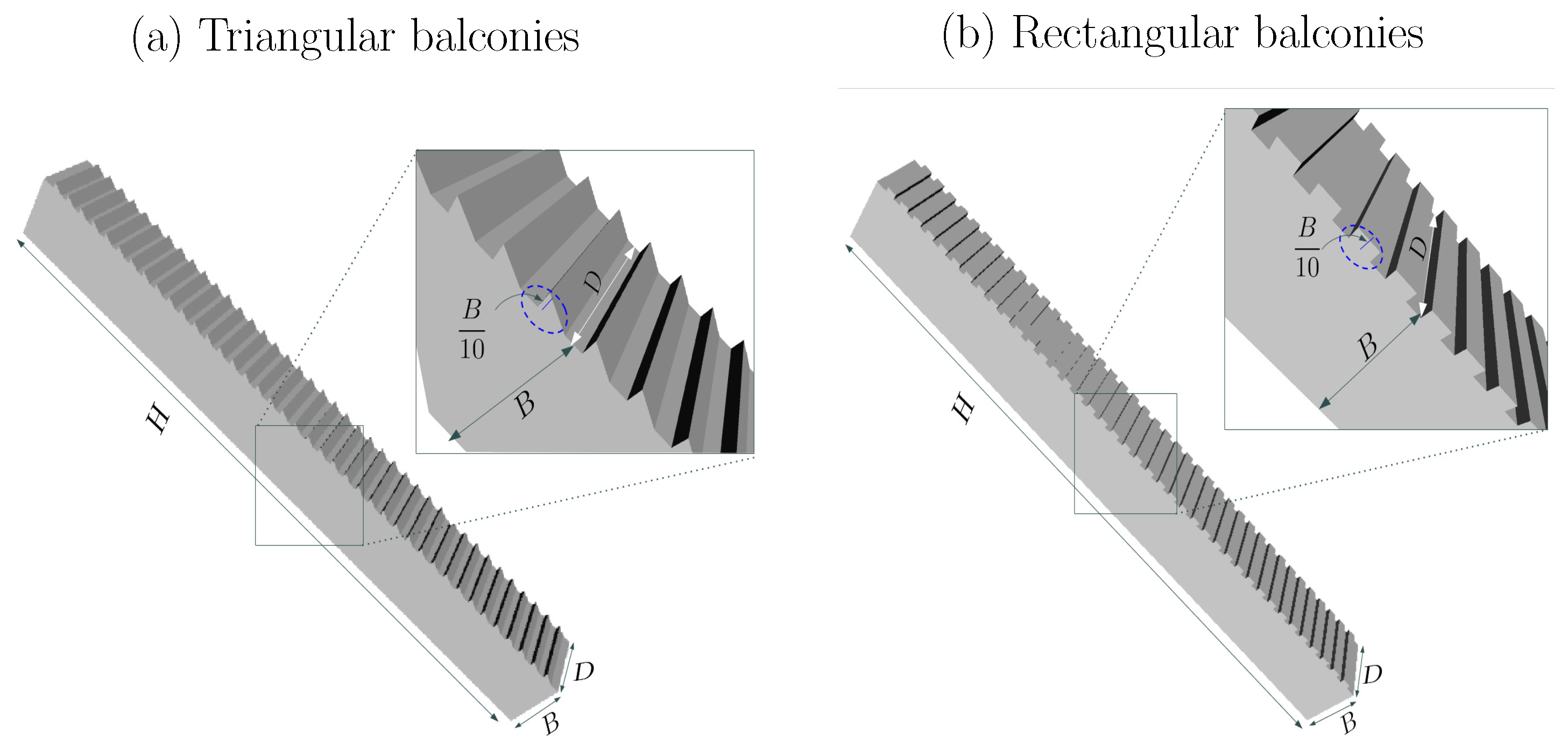
• Buildings considering (i) two types of balconies, (ii) equally spaced (40 floors), (iii) with fixed depth, (iv) without parapet walls or divisions, (v) located at the front, side and rear facades.
• Analysis focused on the averaged values of pressure $C{p}_{avg}$ and vorticity ${\Omega }_{avg}$ around the buildings

4. Numerical Results

Figure 7 and Figure 8 show the maps of average pressure coefficient ($C{p}_{avg}$) and magnitude of vorticity (${\Omega }_{avg}$) recorded at the frontal face of the seven buildings configurations introduced in Section 3.1. Cases (a), (f) and (g) represent the same situation, a flow incident on a smooth surface; cases (d) and (e) also have a smooth surface but with lateral protuberances; cases (b) and (c) receive the mainstream wind load on their balconies.

Figure 9 and Figure 10 show equivalent results for the lateral face (where balconies there exist for cases T90 and R90), and Figure 11 and Figure 12 show the results obtained at the rear face. Note, that the coordinates are expressed in dimensionless form after normalising them with the characteristic length B.

In Figure 7, a maximum pressure ($C{p}_{avg}\approx 0.85$) at the centre line of the facade around a normalised height of 6–9 is observed. From this point the pressure decreases up to a zero value ($C{p}_{avg}=0$) at the corners. One must note that around the pedestrian zone, the pressure slightly increases back again, see for example Figure 7a. Figure 8a, which refers to vorticity, shows the inverse behaviour: fewer vortexes shed at the centre line of the facade but more at the borders. Buildings with balconies at the frontal side, T0 and R0, show zig-zag pattern disturbances at the irregular borders which become more noticeable at the top and bottom of the building. These precise configurations show more extended regions of high (pressure) and low (vorticity) as well as an early flow separation at the building top, which is accompanied by low pressure and vorticity, which are associated with the roughness created by the balconies. As expected, buildings T180 and R180, which have no balconies on the front facade, present little variations with respect to the smooth case. Similar results are seen for cases T90 and R90 which, however, prolong the reduction in $C{p}_{avg}$ and the increase in ${\Omega }_{avg}$ along the position of the lateral protuberances.

When looking at the lateral facades, one can confirm the asymmetric force distributions that characterise flow detachment. This is evident in Figure 9 and Figure 10 for building types T90 and R90, which show a force decrease around the mid-height of these buildings in comparison with the smooth case. In these results, it is also observed that the triangular and rectangular balconies help to mitigate forces around the lateral pedestrian zone ($z/B<0.5$, the first 10 m). Cases (b) and (f) also present a significant local reduction of $C{p}_{avg}$ above $z/B\approx 8$ (160 m) compared with the smooth case. In turn, the high vorticity seen in other building facades is slightly lower with the balconies on T90 and R90, including at pedestrian level; the former does not show great improvements with respect to the smooth facade. Slight zig-zag patterns of pressure and vorticity are also seen for T90 and R90.

As seen in Figure 11 and Figure 12, forces at the rear facade vary across all building types but the best performance is seen on R0, T90 and R180 which show the lowest suction. Notably, T0 tends to increase the suction level at the top of the structure whereas, in terms of vorticity, the best performances are seen for buildings T180 and R180 including at pedestrian level for which T180 seems to provide the best experience. In more detail, cases T180 and R180 result in the zig-zag pattern but change in the distribution of vorticity: larger vorticity values in the lower quarter of the building for the case of triangular balconies, while the larger values are located in the third quarter for rectangular balconies.

The pressure and vorticity maps highlight interesting aspects of performance that could help to identify regions across the building envelope that could, in turn, be susceptible to exceeding target performance levels.

Table 4. Comparison of the main affected zones by the perturbed flow for each building case, in accordance to Figure 7, Figure 8, Figure 9, Figure 10, Figure 11 and Figure 12. Key: F: Front; S: Side; R: Rear; ZZ: zig-zag; SM: smooth; E: equivalent; L: lower; H: higher.

	Location of Roughness	${\mathit{Cp}}_{\mathit{avg}}/{\mathbf{\Omega }}_{\mathit{avg}}$ Pattern Front	${\mathit{Cp}}_{\mathit{avg}}/{\mathbf{\Omega }}_{\mathit{avg}}$ Pattern Side	${\mathit{Cp}}_{\mathit{avg}}/{\mathbf{\Omega }}_{\mathit{avg}}$ Pattern Rear	${\mathit{Cp}}_{\mathit{avg}}$ Amplitude Front	${\mathit{Cp}}_{\mathit{avg}}$ Amplitude Sides	${\mathit{Cp}}_{\mathit{avg}}$ Amplitude Rear	${\mathbf{\Omega }}_{\mathit{avg}}$ Amplitude Front	${\mathbf{\Omega }}_{\mathit{avg}}$ Amplitude Sides	${\mathbf{\Omega }}_{\mathit{avg}}$ Amplitude Rear
T0	F	ZZ	SM	SM	E	L	L	E	H	H
R0		ZZ	SM	SM	E	L	L	E	H	E
T90	S	SM	ZZ	SM	E	L	L	E	L	E
R90		SM	ZZ	SM	E	L	E	E	L	E
T180	R	SM	SM	ZZ	E	E	E	E	E	L
R180		SM	SM	ZZ	E	E	L	E	E	L

shows a summary that compares the main average local flow disturbs. From it, surface roughness tends to induce zig-zag patterns on the facade where balconies lie. It also shows that whereas little changes are observed in the aerodynamics on the front facade (for T90, R90, T180 and R180), the presence of balconies tends to improve or match performances at the side and rear walls. In some cases (see ${\Omega }_{avg}$ for T0 and R0) induce higher vorticity at the side and rear of the building which, as per $C{p}_{avg}$ values, decreases aerodynamic forces.

Following the estimation of local effects, average and RMS force coefficients were determined, which connects with Table 4. They are shown in Figure 13, where the flow disturbances induced by balconies spread across the front facade reduce average drag by about 3% on T0 and by 5.5% on R0. On T90, T180 and R180 lower variations are observed, while on R90 drag force increases in about 6%—considering the same frontal area (R90 produces an increase in drag of about 2% if a frontal area correction is applied). Notwithstanding the large fluctuations observed on R90 and T180, lateral forces do not show significant changes in comparison to the smooth case. This statement is supported by Figure 14 and Figure 15, which show the fluctuating pressure on the lateral and rear faces, respectively, of the buildings. As seen in the panels, no significant variation is reached, although the increasing values of (i) R90 and T180 in the middle zone of the lateral face, and (ii) R90 in the lower zone of the rear face.

5. Discussion

The results obtained highlight benefits and drawbacks derived from the presence of balconies which must be attended to by designers. On the one hand, one can observe an improvement in the aerodynamics around the mid-height of the building where the vortex shedding lowers aerodynamic forces at the corners and centre line, particularly on lateral and rear facades. But on the other hand, across the same lateral and rear facades, higher suction forces are observed at the top of the building, which allows to recommend facades with lower surface roughness at the top quartile of tall buildings. If balconies must be in place at the critical regions then windows, panels, and any non-structural elements must have higher safety factors to avoid failure.

Regarding the shape of the balcony, i.e., triangular vs rectangular did not highlight qualitative differences. The pressure distribution and vorticity are similar in either facade, whereas the magnitude of the observed values remained within $\pm 10$% in all cases and locations without a clear distinction, with the exceptions of (i) the large variations seen on the middle-upper rear facade by T0 and R0, see Figure 11b and Figure 12b and (ii) cases (f) T180 and (g) R180 along the same facade, the former showing larger vorticity values in the lower quarter of the building, while the latter producing similar values but in the third quarter.

In particular, the resulting zig-zag pattern of $C{p}_{avg}$ has been also observed in previous experimental works and CFD simulations dealing with middle and low-rise buildings, such as those carried out by [6,19,20,21,40], and in the systematic analysis of various geometrical arrangements of balconies in a 48 m height building performed by [21]. Therefore, the findings of this research agree, in general, with the references above but for a high-rise building, which allows us to capture larger effects at the top part of the frontal and rear facades that could be attributable to strong winds and the accumulation of loads in the middle parts, see cases T0 and R0 in Figure 7, Figure 8, Figure 11 and Figure 12. A complete comparison around the building is limited since most of those works focus on the study of the facade in which balconies are directly implemented. In turn, a comparison of results for cases T90, R90, T180 and R180 is difficult due to previous results considering azimuths up to ${45}^{\circ }$ from the front face. Nevertheless, this highlights the novelty in knowledge from the present study.

On the other hand, the proposed T0 and R0 facades tend to mitigate high pressure and vortex shedding at the corners. This also agrees with results using similar balconies, like those from [21]; however, it contrasts with experiments implementing balcony parapet walls and/or separated balconies [19], which lead to increased pressure load inside balconies on the lower part flanks.

6. Conclusions

This investigation aligns with on-going developments aiming to shape a modern wind design philosophy focused on performance. The results presented here aim to enhance our understanding of the aerodynamics of tall buildings with additional surface roughness on the front, side, and rear facades. The work differs from previous investigations that covered low- to medium-rise buildings with magnified roughness on single facades. The investigation also distinguishes from previous computational models through a more detailed simulation of the atmospheric boundary layer including proper calibration of turbulence intensity according to the roughness of the surrounding area and height. Wind actions were established through the simulation of wind gusts of 3 min and 20 m/s wind speed acting on tall buildings of $20\times 20\times 200$ m³, whose facades configured with equispaced triangular and rectangular shapes that resemble balconies. The main characteristic of the addition of balconies is the appearance of irregular (zig-zag) patterns on pressure and vorticity fields. There is a slight reduction in the drag forces on the front facade and a notable reduction on side and rear walls when balconies distribute across the front and lateral facades. The presence of balconies on side and rear facades also mitigate vorticity across those areas but notably, while vortex shedding helps to mitigate forces on the front, particularly at the corners.

With the purpose of highlighting other key findings, we summarise the results obtained with the following remarks:

• Buildings with balconies on their frontal face (T0 and R0) produce the largest local variations, producing a zig-zag pattern and reducing high pressure and vortex shedding at the corners, as long as they also reduce drag.
• In contrast with this, balconies on the lateral face (T90 and R90) only affect the distribution on their corresponding lateral faces but are the ones that most increase drag. From the frontal view of the building, pressure on the lateral side of the balconies is also reduced, while vorticity is increased. They also improve the building performance on its lateral face at pedestrian level.
• Balconies on the rear face (T180 and R180) produce similar variations than T0 and R0 on the face they are located.
• The use of triangular or rectangular balconies does not have a significant qualitative impact, causing only variations of no more than 10% for all the cases and locations, with exception of cases T0-R0 on the middle-upper part of the rear facade for both variables, and T180-R180 along the same facade but only vorticity.
• The observed zig-zag patterns agree with similar experiments considering middle and low-rise buildings, extending that previous knowledge to high-rise buildings while observing larger variations on the upper zones.

The evidence generated enables us to better understand how the presence of balconies modify the aerodynamics of buildings. In some areas, forces are mitigated due to more active vorticity whereas in others there is some pressure concentration, like that observed on the middle-top of the building. The latter could lead designers to configure building facades to avoid adverse effects, for example, by lowering roughness at the top of buildings or, if uniform facades must be used, then consider embedding mechanisms for energy harvesting, such as micro-wind turbines distributed on the roof or facades. Ultimately, it is concluded that passive control systems could expand in various ways to achieve target performances like those sought by new design philosophies, which are currently under development.

References

1. American Society of Civil Engineers. Prestandard for Performance-Based Wind Design; American Society of Civil Engineers: Reston, VA, USA, 2019. [Google Scholar] [CrossRef]
2. American Society of Civil Engineers. Minimum Design Loads and Associated Criteria for Buildings and Other Structures, ASCE/SEI 7-16; American Society of Civil Engineers: Reston, VA, USA, 2017. [Google Scholar] [CrossRef]
3. Stathopoulos, T.; Zhu, X. Wind pressures on building with appurtenances. J. Wind Eng. Ind. Aerodyn. 1988, 31, 265–281. [Google Scholar] [CrossRef]
4. Maruta, E.; Kanda, M.; Sato, J. Effects on surface roughness for wind pressure on glass and cladding of buildings. J. Wind Eng. Ind. Aerodyn. 1998, 74–76, 651–663. [Google Scholar] [CrossRef]
5. Yuan, K.; Hui, Y.; Chen, Z. Effects of facade appurtenances on the local pressure of high-rise building. J. Wind Eng. Ind. Aerodyn. 2018, 178, 26–37. [Google Scholar] [CrossRef]
6. Hui, Y.; Yuan, K.; Chen, Z.; Yang, Q. Characteristics of aerodynamic forces on high-rise buildings with various façade appurtenances. J. Wind Eng. Ind. Aerodyn. 2019, 191, 76–90. [Google Scholar] [CrossRef]
7. Shiba, K.; Mase, S.; Yabe, Y.; Tamura, K. Active/passive vibration control systems for tall buildings. Smart Mater. Struct. 1998, 7, 588. [Google Scholar] [CrossRef]
8. Oruç, V. Passive control of flow structures around a circular cylinder by using screen. J. Fluids Struct. 2012, 33, 229–242. [Google Scholar] [CrossRef]
9. Hu, G.; Hassanli, S.; Kwok, K.; Tse, K. Wind-induced responses of a tall building with a double-skin façade system. J. Wind Eng. Ind. Aerodyn. 2017, 168, 91–100. [Google Scholar] [CrossRef]
10. Hou, F.; Sarkar, P.P.; Alipour, A. A novel mechanism—Smart morphing façade system—To mitigate wind-induced vibration of tall buildings. Eng. Struct. 2023, 275, 115152. [Google Scholar] [CrossRef]
11. Jafari, M.; Alipour, A. Methodologies to mitigate wind-induced vibration of tall buildings: A state-of-the-art review. J. Build. Eng. 2021, 33, 101582. [Google Scholar] [CrossRef]
12. Phillips, D.A.; Soligo, M.J. Will CFD Ever Replace Wind Tunnels for Building Wind Simulations? Int. J. High-Rise Build. 2019, 8, 107–116. [Google Scholar] [CrossRef]
13. Thordal, M.S.; Bennetsen, J.C.; Koss, H.H.H. Review for practical application of CFD for the determination of wind load on high-rise buildings. J. Wind Eng. Ind. Aerodyn. 2019, 186, 155–168. [Google Scholar] [CrossRef]
14. Huang, S.; Li, Q.; Xu, S. Numerical evaluation of wind effects on a tall steel building by CFD. J. Constr. Steel Res. 2007, 63, 612–627. [Google Scholar] [CrossRef]
15. Bairagi, A.; Dalui, S. Estimation of Wind Load on Stepped Tall Building Using CFD Simulation. Iran. J. Sci. Technol. Trans. Civ. Eng. 2021, 45, 707–727. [Google Scholar] [CrossRef]
16. Verma, S.K.; Roy, A.K.; Lather, S.; Sood, M. CFD Simulation for Wind Load on Octagonal Tall Buildings. Int. J. Eng. Trends Technol. 2015, 24, 211–216. [Google Scholar] [CrossRef]
17. Ivánková, O.; Hubová, O.; Macák, M.; Vojteková, E.; Konečná, L.B. Wind Pressure Distribution on the Façade of Stand-Alone Atypically Shaped High-Rise Building Determined by CFD Simulation and Wind Tunnel Tests. Designs 2022, 6, 77. [Google Scholar] [CrossRef]
18. Goyal, P.K.; Kumari, S.L.; Singh, S.; Saroj, R.K.; Meena, R.K.; Raj, R. Numerical Study of Wind Loads on Y Plan-Shaped Tall Building Using CFD. Civ. Eng. J. 2022, 8, 263–277. [Google Scholar] [CrossRef]
19. Montazeri, H.; Blocken, B. CFD simulation of wind-induced pressure coefficients on buildings with and without balconies: Validation and sensitivity analysis. Build. Environ. 2013, 60, 137–149. [Google Scholar] [CrossRef]
20. Zheng, X.; Montazeri, H.; Blocken, B. CFD simulations of wind flow and mean surface pressure for buildings with balconies: Comparison of RANS and LES. Build. Environ. 2020, 173, 106747. [Google Scholar] [CrossRef]
21. Zheng, X.; Montazeri, H.; Blocken, B. CFD analysis of the impact of geometrical characteristics of building balconies on near-façade wind flow and surface pressure. Build. Environ. 2021, 200, 107904. [Google Scholar] [CrossRef]
22. Murakami, S. Preface. J. Wind Eng. Ind. Aerodyn. 1990, 35, ix–xi. [Google Scholar] [CrossRef]
23. Prianto, E.; Depecker, P. Characteristic of airflow as the effect of balcony, opening design and internal division on indoor velocity: A case study of traditional dwelling in urban living quarter in tropical humid region. Energy Build. 2002, 34, 401–409. [Google Scholar] [CrossRef]
24. Ai, Z.T.; Mak, C.M.; Niu, J.L. Numerical investigation of wind-induced airflow and interunit dispersion characteristics in multistory residential buildings. Indoor Air 2013, 23, 417–429. [Google Scholar] [CrossRef] [PubMed]
25. Ai, Z.T.; Mak, C.M. Large eddy simulation of wind-induced interunit dispersion around multistory buildings. Indoor Air 2016, 26, 259–273. [Google Scholar] [CrossRef]
26. Llaguno-Munitxa, M.; Bou-Zeid, E.; Hultmark, M. The influence of building geometry on street canyon air flow: Validation of large eddy simulations against wind tunnel experiments. J. Wind Eng. Ind. Aerodyn. 2017, 165, 115–130. [Google Scholar] [CrossRef]
27. Omrani, S.; Garcia-Hansen, V.; Capra, B.; Drogemuller, R. On the effect of provision of balconies on natural ventilation and thermal comfort in high-rise residential buildings. Build. Environ. 2017, 123, 504–516. [Google Scholar] [CrossRef]
28. Kahsay, M.T.; Bitsuamlak, G.T.; Tariku, F. CFD simulation of external CHTC on a high-rise building with and without façade appurtenances. Build. Environ. 2019, 165, 106350. [Google Scholar] [CrossRef]
29. Karkoulias, V.; Marazioti, P.; Georgiou, D.; Maraziotis, E. Computational Fluid Dynamics modeling of the trace elements dispersion and comparison with measurements in a street canyon with balconies in the city of Patras, Greece. Atmos. Environ. 2020, 223, 117210. [Google Scholar] [CrossRef]
30. OpenFOAM. OpenCFD Release OpenFOAM, v2012; OpenCFD Ltd.—ESI Group: Bracknell, UK, 2020. [Google Scholar]
31. Vuppala, R.K.S.S.; Krawczyk, Z.; Paul, R.; Kara, K. Modeling advanced air mobility aircraft in data-driven reduced order realistic urban winds. Sci. Rep. 2024, 14, 383. [Google Scholar] [CrossRef]
32. Elfverson, D.; Lejon, C. Use and Scalability of OpenFOAM for Wind Fields and Pollution Dispersion with Building- and Ground-Resolving Topography. Atmosphere 2021, 12, 1124. [Google Scholar] [CrossRef]
33. Mohan, R.; Sundararaj, S.; Thiagarajan, K.B. Numerical simulation of flow over buildings using OpenFOAM®. AIP Conf. Proc. 2019, 2112, 020149. [Google Scholar] [CrossRef]
34. Spalart, P.; Allmaras, S. A one-equation turbulence model for aerodynamic flows. In Proceedings of the 30th Aerospace Sciences Meeting and Exhibit, Reno, NV, USA, 6–9 January 1992; American Institute of Aeronautics and Astronautics: Reston, VA, USA, 1992; pp. 1–22. [Google Scholar] [CrossRef]
35. Spalart, P.R.; Deck, S.; Shur, M.L.; Squires, K.D.; Strelets, M.K.; Travin, A. A New Version of Detached-eddy Simulation, Resistant to Ambiguous Grid Densities. Theor. Comput. Fluid Dyn. 2006, 20, 181–195. [Google Scholar] [CrossRef]
36. OpenFOAM. Spalart-Allmaras Delayed Detached Eddy Simulation (DDES), v2012; OpenCFD Ltd.—ESI Group: Bracknell, UK, 2020. [Google Scholar]
37. OpenFOAM. Spalart-Allmaras Detached Eddy Simulation (DES), v2012; OpenCFD Ltd.—ESI Group: Bracknell, UK, 2020. [Google Scholar]
38. OpenFOAM. pisoFOAM Solver, v2112; OpenCFD Ltd.—ESI Group: Bracknell, UK, 2018. [Google Scholar]
39. OpenFOAM. ATM Boundary Layer, v2112; OpenCFD Ltd.—ESI Group: Bracknell, UK, 2018. [Google Scholar]
40. Liu, J.; Hui, Y.; Yang, Q.; Tamura, Y. Flow field investigation for aerodynamic effects of surface mounted ribs on square-sectioned high-rise buildings. J. Wind Eng. Ind. Aerodyn. 2021, 211, 104551. [Google Scholar] [CrossRef]
Figure 1. Scheme of the buildings with triangular (a) and rectangular (b) balconies. Size of balconies are defined by their circumscribed radius depending of the characteristic length B of the problem.
Buildings 14 01514 g001
Figure 2. Scheme of the computational array identifying its dimensions, the location of the building and the boundary conditions.
Buildings 14 01514 g002
Figure 3. The visualisation of the mesh refinement for the building with triangular balconies at the front side. (a) 2D view of the delimitation of the six refinement levels labeled with colors. Refinement increases as the cells are closer to the building: the coarsest zone (blue) is defined by l = 0 , producing a cell level of c 0 = 10 m; then, l = 1 (purple) produces c 1 = 5 m, l = 2 (cyan) produces c 2 = 2.5 m, l = 3 (green) produces c 3 = 1.25 m, l = 4 (yellow) produces c 4 0.63 m, and the finest zone l = 5 (red) produces c 5 0.31 m. (b) 3D zoom visualisation of the bottom part of the building, with l = 5 ( c 5 0.16 m) at its surface and the decreasing refinement of the terrain as it moves away from the building.
Buildings 14 01514 g003
Figure 4. Inflow boundary profiles of U x and I, according to Equations (5)–(7) and Table 2.
Buildings 14 01514 g004
Figure 5. Comparison of pressure coefficient around the smooth building at 2 3 H . The auxiliary variable of distance ξ goes around the building as illustrated in the inside draw. (a) Average. (b) RMS.
Buildings 14 01514 g005
Figure 6. Comparison of time series produced by M2, considering 3 min of wind simulation (black) and 10 min (black + blue). (a) Drag coefficient. (b) Lateral coefficient.
Buildings 14 01514 g006
Figure 7. Color maps of average pressure C p a v g at the frontal face of the buildings: (a) smooth; (b) T0-facade with triangular balconies; (c) R0-facade with rectangular balconies; (d) T90-triangular balconies in one the lateral side; (e) R90-rectangular balconies in one lateral side; (f) T180-triangular balconies in the rear side and (g) R180-rectangular balconies in the rear side of the building. Cases (a,f,g) represent the same situation, a flow including on a smooth surface. Cases (b,c) follow a horizontal striped pattern (zig-zag)—in these cases the pressure on the upper zone of the building is significantly reduced. Cases (d,e) show a reduction in pressure along the position of the lateral protuberances.
Buildings 14 01514 g007
Figure 8. Color maps of average vorticity Ω a v g at the frontal face of the buildings—the cases correspond to those in Figure 7: (a) smooth, (b) T0, (c) R0, (d) T90, (e) R90, (f) T180, (g) R180. In all cases, vorticity increases from the centreline of the facade to the lateral sides. In this respect, cases (a,dg) are similar. The presence of the roughness produces a zig-zag pattern along the vertical centreline, cases (b,c).
Buildings 14 01514 g008
Figure 9. Color maps of C p a v g on the lateral face, then the flow goes from left to right in all panels—the cases correspond to those in Figure 7: (a) smooth, (b) T0, (c) R0, (d) T90, (e) R90, (f) T180, (g) R180. Cases (b,f) present a significant increase in (negative relative) pressure above z / B = 8 (160 m) compared with the smooth case (a). For cases (d,e), the map in the upper half of the building shows a very smooth zig-zag pattern that resembles a crocodile tail pattern, due to the presence of balconies—these two cases also have lower values of pressure for z / B < 0.5 , the first 10 m (the pedestrian zone). On the other hand, cases (be) present a general decrease in the middle zone of their corresponding building. Roughly speaking, cases (f,g) are close to the solution for the smooth case (a), even though the increase in pressure in the upper zone for case (f).
Buildings 14 01514 g009
Figure 10. Color maps of average vorticity Ω a v g on the lateral face - the cases correspond to those in Figure 7: (a) smooth, (b) T0, (c) R0, (d) T90, (e) R90, (f) T180, (g) R180. A small extension of the high vorticity values in the middle-upper zone is obtained by balconies on the front side, cases (b,c). Balconies located on the lateral facade, (d,e), produce a striped pattern and a global reduction in vorticity. No significant changes are obtained by using balconies in the rear side, cases (f,g).
Buildings 14 01514 g010
Figure 11. Color maps of average pressure C p a v g on the rear face, then the flow goes from inside to outside of the page in all panels - the cases correspond to those in Figure 7: (a) smooth, (b) T0, (c) R0, (d) T90, (e) R90, (f) T180, (g) R180. Leaving aside the details, cases (ae) give similar distributions of pressure, although with significantly higher values on the upper zone for case (b), and lower values in the middle zone for cases (bd). Cases (f,g) result in the zig-zag pattern, the pressure value in the stripes along the vertical is strongly affected by the type of balcony.
Buildings 14 01514 g011
Figure 12. Color maps of average vorticity Ω a v g on the rear face - the cases correspond to those in Figure 7: (a) smooth, (b) T0, (c) R0, (d) T90, (e) R90, (f) T180, (g) R180. Cases (ae) produce a similar behavior, presenting large values of vorticity close to the border of the upper half of the buildings, with a larger effect for case (b) above at z / B = 6 (120 m). The lower values in the vertical center line of the smooth case (a) are also cut by the cases with balconies (be) around z / B = 6 7 . Cases (f,g) show the effect of balcony shape (triangle vs. square) in the distribution of vorticity, larger vorticity values in the lower quarter of the building in the case of triangular balconies, while greater values in the third quarter in the case of rectangles.
Buildings 14 01514 g012
Figure 13. Drag (blue) and lateral (red) coefficients for the considered buildings. Average values with dots and RMS values with error bars.
Buildings 14 01514 g013
Figure 14. Color maps of fluctuation pressure C p s t d on the lateral face, then the flow goes from left to right of the page in all panels—the cases correspond to those in Figure 7: (a) smooth, (b) T0, (c) R0, (d) T90, (e) R90, (f) T180, (g) R180.
Buildings 14 01514 g014
Figure 15. Color maps of fluctuation pressure C p s t d on the rear face, then the flow goes from inside to outside of the page in all panels—the cases correspond to those in Figure 7: (a) smooth, (b) T0, (c) R0, (d) T90, (e) R90, (f) T180, (g) R180.
Buildings 14 01514 g015