Abstract
Seismic vulnerability assessment in urban areas would, in principle, require the detailed modeling of every single building and the implementation of complex numerical calculations. This procedure is clearly difficult to apply at an urban scale where many buildings must be considered; therefore, it is essential to have simplified, but at the same time reliable, approaches to vulnerability assessment. Among the proposed strategies, one of the most interesting concerns is the application of machine learning algorithms, which are able to classify buildings according to their vulnerability on the basis of training procedures applied to existing datasets. In this paper, machine learning algorithms were applied to a dataset which collects and catalogs the structural characteristics of a large number of buildings and reports the damage observed in L’Aquila territory during the intense seismic activity that occurred in 2009. A combination of a trained neural network and a random forest algorithm allows us to identify an opportune “a-posteriori” vulnerability score, deduced from the observed damage, which is compared to an “a-priori” vulnerability one, evaluated taking into account characteristic indexes for building’s typologies. By means of this comparison, an inverse approach to seismic vulnerability assessment, which can be extended to different urban centers, is proposed.
1. Introduction
Several countries around the world have large territories characterized by the presence of buildings not designed according to seismic codes and, therefore, unsuitable to resist possible earthquakes. Therefore, a crucial aspect lies in the assessment of the seismic vulnerability of existing buildings, which can be performed by means of detailed individual models or simplified methods at an urban scale. The seismic vulnerability assessment of single buildings requires a deep knowledge of the structure and involves the construction of accurate numerical models. Since the task is very demanding, several simplified models of buildings have been analyzed in recent decades [1,2,3,4,5]. Although simplified, these approaches involve the execution of difficult calculations and, therefore, cannot be applied at the urban scale where a great number of buildings must be analyzed, and a fast, although reliable, vulnerability assessment is crucial in identifying the areas most exposed to seismic risk in which to intervene as a priority.
With this aim, many simplified methods for seismic vulnerability assessment at the urban scale have been presented in the scientific literature. For example, rapid visual screening (RVS) is a qualitative estimation procedure which can be used to classify the vulnerability of structures by means of observations made from the building exterior without taking into consideration the building inside [6]. This visual survey can be considered the first step in the vulnerability assessment for determining the risk priorities for buildings before going into further detail and classifying them according to their construction materials and structural systems. Other methodologies, called vulnerability index methods (VIM), are based on the estimation of some characteristic indexes. These approaches rely on the knowledge of a large number of damage survey data and structural information in order to investigate the influence of different parameters on the seismic vulnerability of the building [7,8]. For instance, they have been applied to seven European cities [9]. The macro-seismic approach combines the vulnerability index method with an analytical function which expresses the expected damage for a given earthquake intensity [10,11,12,13]. Another popular method is based on the damage probability matrix [14,15,16], which returns an estimate of vulnerability in numeric form; in particular, it expresses the likelihood of a certain level of damage for each seismic intensity. This method provides the seismic vulnerability as an estimation of the probability of occurrence of damage in buildings in terms of the intensity of the earthquake.
Several studies on seismic vulnerability at the urban scale follow a mechanical approach based on the consideration of ideal numerical models of existing building typologies [17] and aggregates of buildings [18]. Recurrent geometrical, structural, and technological features of buildings can be identified using the geographic information system [19]. Geometrical and mechanical uncertainties are modeled using information derived from available databases.
Since seismic assessment at an urban scale involves the use of a great amount of data, many of which are repeated for similar buildings, an interesting and promising approach is based on machine learning algorithms (MLA). These algorithms allow us to produce reliable results through a learning process applied to opportune training datasets, making precise predictions about new data. MLA, formerly of specific interest to computer scientists, have been largely developed in recent decades and applied to several engineering research fields. In recent years, a wide range of applications have been found in structural engineering since the algorithms are useful in dealing with problems associated with uncertainties due to their effectiveness and robustness in dealing with noise.
Several applications of MLA to seismic vulnerability analyses at the urban scale have been developed. For example, applications of an artificial neural network (ANN) model [20] and of a SWOT-quantitative strategic planning matrix (QSPM) [21] have been recently developed for the evaluation of seismic vulnerability in different municipalities in Iran. Other studies evaluated the seismic vulnerability of large sets of buildings in urban environments through a procedure based on the fast calculation of capacity curves of low-rise reinforced concrete buildings using neural networks [22]. Building capacity curves for 256 reinforced concrete buildings with between four and seven floors were obtained in [23], where the influence of the structural parameters on the seismic performance was quantified using a set of artificial neural network algorithms. In [24], the assessment of the vulnerability of urban blocks to earthquakes using an artificial neural network–multi-layer perceptron (ANN-MLP) was presented. To train the neural network and compute earthquake vulnerability maps, a combined multi-criteria decision analysis (MCDA) process was adopted. A combination of artificial neural network-based predictive models and decision-making methods based on a hierarchy process with the aim of improving the earthquake risk assessment was presented in [25,26] and applied to a city in Indonesia. They identified the major indicators required to create reliable vulnerability maps in seismic risk assessment. In particular, in [26], artificial neural networks were also used to train and optimize a database of 145 damaged buildings from the Haiti earthquake. The comparison between the performances of artificial neural networks and traditional regression models in the evaluation of the seismic vulnerability of a large set of buildings was presented in [27]. A hybrid approach of machine learning (random forest) and hierarchical analysis (Saaty matrix) was used for the seismic risk assessment of the Peruvian city of Pisco [28], and a double-entry table relating hazard and vulnerability levels was presented. Frequency ratio (FR), decision tree (DT), and random forest (RF) methods were also applied to seismic data for Gyeongju, South Korea, in [29]. Machine learning techniques were recently applied to define damage classification boundaries using data from six post-earthquake damage surveys [30] and predict the level of damage to reinforced concrete buildings by means of developed platform applications [31]. MLAs have also been applied to provide an indication of the seismic vulnerability of urban areas by exploiting building data from photographs [32]. Foresight into the damaged state of reinforced concrete buildings using ANN using databases from the Nepal and Ecuador earthquakes was presented in [33].
In this paper, our main goal is to calculate, through an opportune combination of a simple, fully connected ANN and a random forest classifier, a seismic vulnerability score for the buildings in a specific urban area based on a dataset reporting the damages produced by multiple seismic events. In particular, the region around the city of L’Aquila, Italy, has been considered in relation to the devastating sequence of earthquakes that occurred in April 2009. Our approach can be considered an inverse problem, according to which the “a posteriori” vulnerability of the buildings is inferred from the observed damages. The features of several buildings (such as date of construction, construction material, number of floors, and floor area) have been identified according to accredited building classification systems [34], and a thorough analysis of the contribution of each feature to overall vulnerability is performed.
Further comparison with another vulnerability score, built according to the main construction features of the buildings available in the chosen dataset and thus denoted as “a priori”, will be performed. From the comparison between these two scores, we can deduce some general trends that allow us to improve and enrich the estimate of the seismic vulnerability of buildings at an urban scale. This proposed procedure represents a flexible, feature-focused tool applicable to seismic vulnerability assessment of different urbanized territories and could be extremely useful in planning appropriate measures for risk management, particularly if combined with further information regarding road infrastructures when available.
2. Buildings Dataset and “a priori” Seismic Vulnerability Estimation
In 2009, a long sequence of seismic events occurred in the Abruzzo region of central Italy (see panels of Figure 1a,b), which can be attributed to its complex tectonic setting. In fact, this region is characterized by the convergence of the African and Eurasian plates that, accompanied by the extension of the Apennine Mountain range, generates significant seismic activity. The considered sequence started in December 2008 and culminated on 6 April 2009, with a main shock of magnitude Mw 6.3 registered at 3:32 AM local time, followed by several aftershocks. This earthquake had an epicenter located near the city of L’Aquila, the capital of the Abruzzo region, and occurred at a shallow depth of approximately 8.8 km, a detail which contributed to the significant damage experienced in the region.
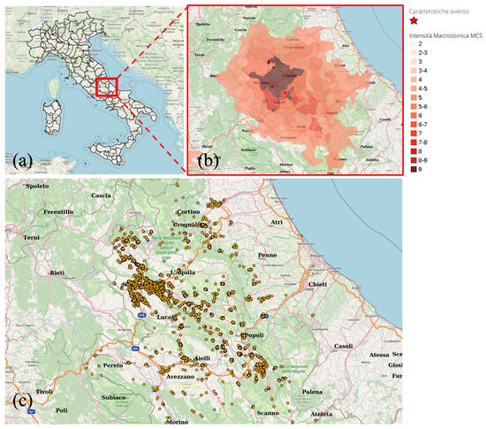
Figure 1.
(a) Map of Italy. (b) An enlargement of the region around L’Aquila reporting the epicenters of the April 6th five main shocks, represented as star symbols (the main event is also marked with a circle), (c) Geographical position of buildings present in the considered dataset [35].
In our analysis, we utilize the extensive Da.D.O. dataset [35], which includes a comprehensive record of 58,140 buildings in the proximity of L’Aquila. This dataset encompasses pre-event characteristics such as age, construction material, and geometry of the buildings, as well as post-event damage assessments following a series of the five most significant earthquakes, each with a magnitude greater than 5 ML that occurred between 6 and 9 April 2009. The epicenters of these earthquakes are represented as red star symbols in the panel of Figure 1b, while the main event of magnitude Mw 6.3 is marked with a circle. The geographical positions of the buildings present in the dataset are depicted in panel Figure 1c, highlighting their distribution in the affected area. Additionally, the data have been georeferenced and converted into shapefile format for effective analyses.
Based on the information reported on the Da.D.O. dataset, an “a priori” vulnerability score for each building in the considered area can be calculated based on the appropriate structural features, as shown in Table 1. This is a categorical score ranging from the maximum level A (highest vulnerability) to the minimum level D2 (lowest vulnerability). This “a priori” score will be later compared with an “a posteriori” one, evaluated on the basis of the observed damages, as explained in the following sections.

Table 1.
“A priori” vulnerability classes of buildings evaluated on the basis of some of their structural features, following the indications present on the Da.D.O web platform [35].
3. Machine Learning Models and Dataset Pre-Processing
The aim of our work is to use the information reported on the dataset for assessing the correlations of building features with damage levels and to propose a new vulnerability score for each building evaluated “a posteriori” on the basis of the observed damage. In this respect, we approached the problem of seismic vulnerability assessment as a multi-class classification task which employs machine learning algorithms.
3.1. ANN and Random Forest Algorithms
We have chosen to focus our study on a classification approach involving two machine learning models: a random forest classifier (RFC) and a custom-designed artificial neural network (ANN) [36,37].
- Random Forest Classifier (RFC): This model is an ensemble learning technique, well-regarded for its robustness and accuracy in various applications. The main key strength of random forest algorithms lies in their ability to prevent overfitting, a common challenge in machine learning models. This is achieved through its ensemble nature (see Figure 2), where multiple trees, each trained on subsets of the data with randomized feature selection, contribute to the final classification, thus ensuring a very reliable performance.
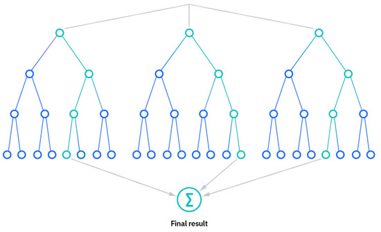 Figure 2. An example of a random forest classification tree [https://www.ibm.com/it-it/topics/random-forest, accessed on 23 November 2023].
 - Artificial Neural Network (ANN): This model is inspired by a brain’s neural networks, comprising layers of interconnected nodes or neurons. Each node processes the input data, which then travel through multiple layers, each altering the input uniquely. ANNs excel in learning intricate patterns in data by modifying the weights of the connections between neurons through backpropagation. Figure 3 shows the architecture of the ANN used in our work: after normalization, the data are passed onto the ‘Feature Augmentation’ module, which applies mathematical transformations to the numeric values (building coordinates and distance to the five main epicenters) in order to improve both the model’s ability to assign the correct vulnerability to each location and the overall performance.
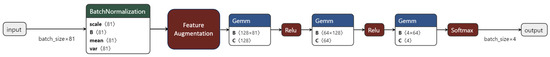 Figure 3. Architecture of the ANN used in our work (numbers in <brackets> record the size of each component): the input is a vector of 81 values combining numerical values with categorical ones. This vector is normalized and passed to a series of general matrix multiplications (Gemm). The feature augmentation module calculates squares and cubes of numeric values, as well as a selectable number of sine and cosine transformations for which the parameters (amplitude, phase frequency, and bias) are learned during training. We use a particular activation function (Relu) to introduce non-linearity in the model. The last layer is a function (Softmax) that normalizes the output to represent probability distribution across the 4 damage classes.
We also employed the one-hot encoding technique to represent categorical data within these machine learning models. This method converts categorical variables into a form that can be provided to ML algorithms to do a better job in prediction. It involves expanding each categorical class into a new binary column, which increases the efficiency of the process. This step is critical in ensuring that categorical data, such as building types or construction materials, are effectively incorporated into our vulnerability assessment models.
3.2. Data Pre-Processing and Features Selection
In the following section, we detail the taxonomy of buildings in our dataset. In order to ensure the compatibility of data with the analysis pipeline, we pre-processed them opportunely. In addition to usual normalization and data cleaning, the main steps were the following two:
- Since the original dataset employs highly detailed damage categorization, some simplification is necessary. First of all, we only refer to damage that occurred in vertical structures. The level of damage was originally classified according to what was proposed in the European Macroseismic Scale EMS-98, namely: D1 (light damage), D2 (moderate damage), D3 (extensive damage), D4 (total damage), and D5 (collapse). The zero damage class D0 was also added to the previous ones for completeness. Since, in the database, damages are reported for different portions of each building, the different combinations result in a complex matrix of 26 distinct damage classes with a non-homogeneous number of elements. To circumvent this issue, we condensed these classes, assuming the highest level of damage sustained by any of its portions for each building. Finally, merging the three highest damage classes (D3, D4, and D5) into a macro class representing general ‘high damage’ reduces the classification to four ordinal damage categories, ranging from D0 to D3. Alternative strategies, like assigning a numerical score to each of the 26 categories for regression analysis or experimenting with different class counts, were explored but did not enhance the model’s performance. This optimized approach is both efficient and practical, ensuring a more balanced and manageable dataset for analysis.
- Then, specific columns (Figure 4) from the original dataset were selected for analysis, including geographic, structural, and damage-related information. The considered characteristics of the buildings concern the following:
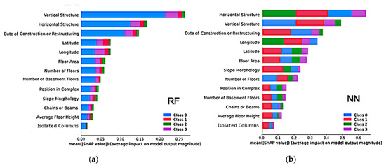 Figure 4. Impact of input features to the output of the proposed models, (a) random forest (RF) and (b) neural network (NN), expressed by the mean of their SHAP values. The output classes are reported in the legend from the one associated with the lower damage level (D0) to that associated with the highest one (D3). For each row (feature) in the bar graph, the classes are ordered from the one which, overall, has been mostly predicted from the model to the one which has been predicted for the least amount of time.
- Horizontal and vertical structure typologies;
- Chains, beams, or isolated columns;
- Year of construction or restructuring;
- Latitude and longitude of buildings;
- Number of floors, basement floors, floor height, and area;
- Slope morphology and position in the complex.
Our goal was to understand how different features influence the decisions of various models, particularly in classifying various levels of damage, in order to see if we can streamline these features.
To select the top predictive features, preliminary models were trained, utilizing the Shapley Additive exPlanations (SHAP) model for both a neural network and random forest. This model, initially introduced by Lloyd Shapley [38], employs game theory to explain the outputs of machine learning models. The core idea of SHAP is based on Shapley values, which calculate the contribution of each subset of features (from a total of ‘m’ features) to the model’s predictions [39]. Specifically, the impact of the ‘i-th’ feature is determined by comparing the predictions of the original model with those of a model trained without the ‘i-th’ feature. Since removing a feature can also affect others, this comparison must be made for every possible subset of features, excluding the ‘i-th’ one. The Shapley value is then the average of these comparison scores. The output of this process is the bar plot shown in Figure 4, where the overall impact of each feature on the prediction task is split into colors representing the contribution to each damage class in the dataset. Thus, SHAP was used to gain insight into which features are linked with specific damage levels, according to our data dataset and models.
From these graphs, it is evident that the random forest model tends to underfit the data and predict a lower level of damage compared to the neural network. Despite some differences in the importance ranking of features, which are expected due to the distinct nature of the two models, the top six influential features were the same for both. These significant features were mainly structural, like the type of vertical and horizontal structures and the construction year, aligning with the predefined vulnerability classes. On the other hand, features like “Chains or Beams”, “Average Floor Height”, and “Isolated Columns”, though part of the predefined vulnerability classes, were not influential in our models. These three less influential features were consistent across both models, allowing us to reduce the total number of input parameters from 13 to 10.
Finally, the data were augmented by pre-calculating the distances of each building from the five main epicenters to allow the model to easily learn the correct vulnerability of each location in the dataset.
4. “A posteriori” Seismic Vulnerability Estimation and Numerical Results
As already anticipated, the core of our analysis is the evaluation, on the basis of the observed damage levels, of an “a posteriori” vulnerability score for each feature present in the dataset, and by extension, for each building. This score is derived from the neural network and random forest models, with an average over the two models’ results taken to mitigate model-specific biases.
The first preliminary step simply involved training these models to predict the damage based on the available dataset information, dividing the data into training and validation sets, and reporting the performance of both models on the validation set (20% of the data).
The results reported in Figure 5 show the performance of both models when tested on the validation dataset; that is, on new data the models had not seen during training. One can see that the ANN achieved higher precision and recall on all classes, being especially capable of identifying the highest damage class (D3—severe damage) when compared to the random forest.
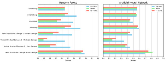
Figure 5.
Performances on validation data (20% of original dataset): we evaluated the standard metrics of precision, recall, and their geometric average, usually named F1 score; precision evaluates the percentage of true positives in classification, while recall is the percentage of buildings of any given class that were identified as such. We evaluated performance in each class and reported various weighted averages.
The second step was dedicated to evaluating the predictive power of our models and establishing the advantages of our vulnerability scoring method. In particular, we introduced an innovative technique to derive an “a posteriori” vulnerability score for each structural feature of the buildings in our dataset. In the following, we show how it works:
- Creation of dummy buildings: these are not real buildings but virtual ones created only for analysis. Each dummy building mirrors the actual buildings in all respects except for one chosen feature, which is held constant across the entire set. For instance, we might simulate a group of buildings with exactly two floors, regardless of their original design.
- Model predictions: we then input these dummy buildings into our pre-trained machine learning models: the neural network and random forest. The models assess each building and output a damage prediction, treating the fixed feature as a variable of interest.
- “A posteriori” vulnerability score derivation: by analyzing the predicted damage across all dummy buildings with the fixed feature, we can calculate an average predicted damage value. This average becomes a numerical representation, a score, of the vulnerability contributed by that specific feature (e.g., having two floors).
- Comprehensive feature analysis: this procedure is methodically applied to each categorical feature within our dataset. As a result, we establish a continuous “a posteriori” vulnerability score for every characteristic examined.
- Score averaging for robustness: to ensure our findings are not skewed by the idiosyncrasies of a single model, we further average the results of the “a posteriori” vulnerability scores obtained with both the neural network and the random forest models. This step enhances the reliability of our results, yielding a more balanced and comprehensive “a posteriori” vulnerability score for each building feature.
By systematically applying this method, we not only assigned a quantifiable score to the elements that contribute to building vulnerability but also provided a scalable approach to assess any number of features. The main advantage of this approach, when compared to traditional Bayesian analysis, is the ability to simultaneously deal with both numeric and categorical data in the evaluation of risk. For example, traditional probabilistic methods require discretization of the coordinate space into finite bins in order to properly define a probability space; instead, our method directly incorporates numerical and categorical variables into the model, bypassing the need for such discretization. This provides a more nuanced and detailed analysis of each feature’s impact on building vulnerability and increases the capability to interpolate a continuous vulnerability map with arbitrary resolution, as detailed in Section 4.1. Furthermore, our approach offers a significant advantage in handling large datasets. Where traditional methods may struggle with computational requirements and scalability issues, our machine learning models, especially the neural network one, can efficiently process and analyze vast amounts of data, allowing for quick fine-tuning in the optimization stage.
4.1. Demonstrating Spatial Independence in Seismic Vulnerability Prediction
As the first application, we showed that this method can be applied to continuous input features, such as building coordinates, by virtually ‘placing’ a batch of dummy buildings across a geographical grid and evaluating their average predicted damage for each location, thus interpolating a continuous vulnerability map that highlights the impact of seismic events within the urban area. The point of this was to show the model’s capacity to differentiate between the inherent vulnerability of individual buildings and the spatial dependency typically associated with seismic risk.
In Figure 6, we show the results of applying this method to our dataset. Maps (A) and (B) represent the vulnerability interpolation across a geographic grid by evaluating the average predicted damage at each grid point using our artificial neural network (ANN) model. The red crosses denote the epicenters of seismic events, with their size proportional to the magnitude of each event. Map (A) shows the results obtained without using the Feature Augmentation module (Figure 3). This provides us with a coarse macroscopic view of risk, highlighting a single zone of high vulnerability correlated with the main epicenters without distinguishing the impact of each one but still validating the model’s effectiveness in recognizing spatial patterns in seismic risk. Map (B) shows the effect of using the feature augmentation module described in Figure 3 to improve mapping ability. This produces a more refined vulnerability map that is able to resolve and distinguish the main epicenters, effectively capturing details that the simpler model misses. The result is a nuanced view of the risk distribution, with the gradations in color on the map indicating varying levels of vulnerability with greater precision. Finally, map (C) overlays the better vulnerability map (B) onto the geographical area. This overlay provides valuable insights into the correspondence of the model’s outputs with real-world locations.
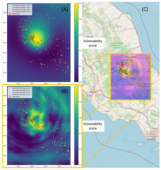
Figure 6.
Vulnerability maps interpolated using the ANN model shown in Figure 3. By placing dummy buildings across a grid and averaging the predicted damage for each location, it is possible to identify high-risk zones, with brighter zones representing high vulnerability (A); vulnerability map interpolated feeding the raw data to the model with no numerical feature augmentation (B): by pre-calculating nonlinear transformations of both the coordinates of buildings and distances from epicenters, using the ‘Feature augmentation’ module described in Figure 3, our model is able to learn a more detailed vulnerability map which is overlayed on the geographical map (C).
4.2. Feature Analysis and A-Posteriori Vulnerability Score
By leveraging the model’s ability to separate spatial dependencies from building vulnerability, we can now finally evaluate a new continuous vulnerability score for each building, which does not depend on its position with respect to the epicenters but exploits the information about observed damages. This point is critical because it allows such “a posteriori” vulnerability score to be potentially useful outside of the location and the events considered in the present study. As already explained, our approach consists of using virtual (dummy) buildings in order to extrapolate the impact of each feature for the prediction of damage. We do this by focusing on one feature at a time and averaging the prediction over a large sample of different buildings with different characteristics and positions but with the same chosen feature. Figure 7 provides a detailed view of the “a posteriori” vulnerability scores for each feature calculated by both the random forest (green bars) and the neural network (red bars) algorithms alongside their average (blue bars).
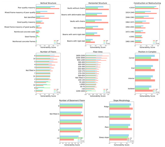
Figure 7.
“A posteriori” vulnerability scores for the 8 considered building features, calculated by both random forest (RF, green bars) and artificial neural network (ANN, red bars) models, highlighting the impact of specific attributes on overall building vulnerability. For each feature, the average score of the two models is also reported (blue bars), representing a more reliable measure of the true features’ vulnerability.
This analysis is instrumental in isolating the contribution of individual building attributes, ranging from the year of construction to employed materials, towards the overall vulnerability. By comparing the scores between models, we can evaluate the consistency of our predictive features, ensuring that our vulnerability assessment is both accurate and reliable.
4.3. Correlation Analysis at Fixed Distance
We aimed to analyze the correlation between various vulnerability metrics and observed damage. To achieve this, we focused on a subset of 13,678 buildings located within 6 km of the five major epicenters. We compared our continuous “a posteriori” vulnerability score with the “a priori” one, which categorizes buildings into five levels of vulnerability, scaled from the maximum level A (highest vulnerability) to the minimum level D2 (lowest vulnerability). This analysis is presented through separate graphical representations due to the different nature (continuous and categorized, respectively) of the two vulnerability scores.
In the bar chart distributions of Figure 8, the frequency of buildings for each damage level is plotted against both our derived “a posteriori” vulnerability score (a) and the “a priori” vulnerability one (b), which can be considered a benchmark. The “a posteriori” vulnerability score typically exhibits a continuous distribution that is more closely aligned with the actual damage levels. This alignment is especially pronounced for the extremes of the damage spectrum (damage levels D0 and D3), showing our method’s enhanced capability to differentiate between the most and least vulnerable structures.
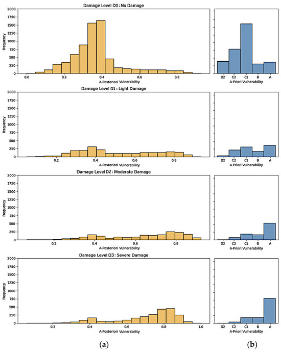
Figure 8.
Distribution bar chart comparing our continuous “a posteriori” vulnerability score (a) with the established categorical “a priori” classification method (b) for the four levels of damage, with a focus on 13,678 buildings within a distance of 6 km from the major epicenters.
In Figure 9, we compare the predictive power of the two methods in a more quantitative way. In panel Figure 9a, the violin plot allows us to appreciate the good linear correlation between the “a posteriori” vulnerability distributions and the observed damage classes, confirmed by the values of both the Spearman and Kendall coefficients reported in the box. On the other hand, in panel Figure 9b, the contingency matrix for the “a priori” vulnerability is reported, where the color gradient of each cell reflects the corresponding number of buildings in the dataset. The matrix shows a less evident correlation with the observed damage, confirmed again by the lower values of the considered coefficients with respect to the “a posteriori” ones. This result further identifies the “a posteriori” vulnerability score as a better predictor of damage, particularly at higher damage levels.
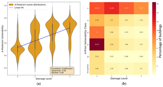
Figure 9.
(a) Violin plot showing the linear correlation between the “a posteriori” vulnerability scores and the observed damage, with good values for both Spearman (0.62) and Kendall (0.48) coefficients. (b) A less evident correlation with the damage emerges from the contingency matrix of the “a priori” vulnerability score, where darker colors indicate a higher percentage of buildings: lower values of Spearman (0.52) and Kendall (0.44) confirm the worse predictive power of this score with respect to the “a posteriori” one.
4.4. Correlation Analysis over Distance
In contrast to the previous section, where we focused on buildings within a 6 km radius of any epicenter, let us now explore the impact of varying this maximum distance. By plotting the Spearman and Kendall correlation coefficients as a function of increasing distances from the epicenters in Figure 10, we effectively illustrate the enhanced accuracy of our vulnerability scoring system.
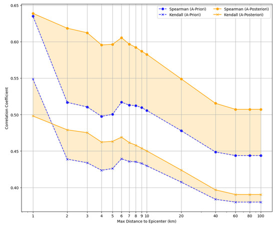
Figure 10.
Spearman and Kendall correlation coefficients plotted against increasing distances from the main earthquakes’ epicenters, illustrating the robustness and accuracy of our “a posteriori” vulnerability scoring system (orange continuous lines) over different proximities, also compared with the “a priori” scores (blue dashed lines).
Looking at the figure, both the “a priori” scores and the derived “a posteriori” ones exhibit a predictable correlation decrease with the increases of the distance from the epicenter, aligning with the expected lower impact of the earthquake. However, our “a posteriori” vulnerability score consistently maintains a notably higher correlation with the damage level, even at large distances. This trend not only underlines the robustness of our approach but also highlights its predictive power in assessing earthquake vulnerability across varying proximities to epicenters.
5. Discussion and Conclusions
Our methodology, as explained in detail in the previous sections, offers a novel and promising approach to seismic vulnerability assessment of buildings in urban areas. The procedure was developed on the basis of the results obtained from a large dataset reporting the damage that occurred in the buildings in the region around L’Aquila (Italy) after the devastating sequence of earthquakes that occurred in April 2009. By focusing on the generation of an “a posteriori” vulnerability score based on the observed damage for each building, we developed a more refined and adaptable tool for seismic vulnerability assessment.
The core of our method lies in the use of machine learning models, specifically a neural network and a random forest classifier, to predict damage based on building features. This approach relies on the introduction of virtual dummy buildings able to assess the impact of individual features on the overall vulnerability, ensuring spatial independence and broad applicability across diverse locations. After a preliminary training of the models with the observed damage data, where geographical information has been used as a bias for separating spatial dependency from building feature analysis, we introduced our “a posteriori” scoring system through the analysis of simulated buildings over various distances from any epicenter. Such an approach showed an improved performance with respect to a more traditional “a priori” method, which assigns categorical vulnerability scores based only on the building’s characteristics. On the contrary, our “a posteriori” method assigns continuous numerical scores to each building, thus allowing for a more detailed and dynamic representation of vulnerability.
Finally, to better appreciate the difference between the two approaches, in Figure 11, we plot the distribution of our “a posteriori” vulnerability score within each “a priori” vulnerability class, from the least vulnerable (D2) to the most vulnerable (A). This visual data representation enables us to discern the considerable improvement in both the quality and the quantity of information yielded by our novel scoring system.
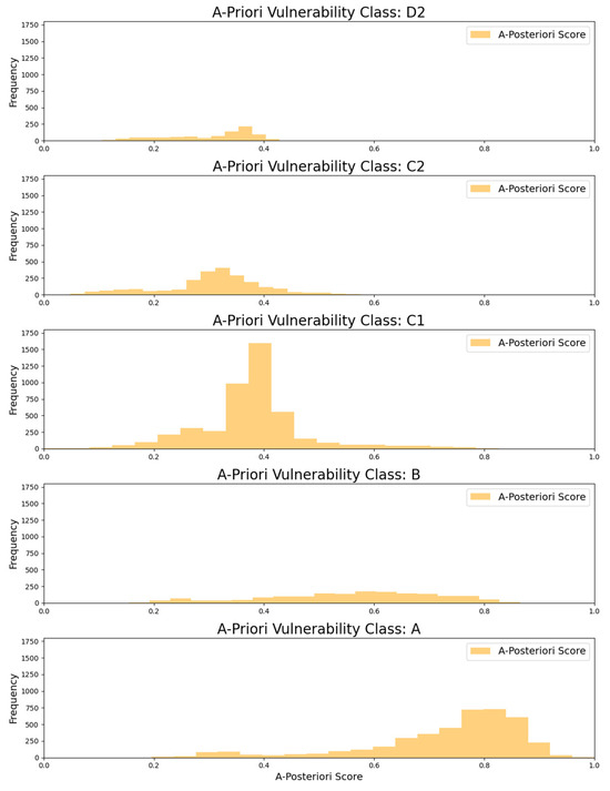
Figure 11.
The distribution of the “a posteriori” vulnerability score is reported for each predefined “a priori” vulnerability category. Here, we clearly observe a wide spectrum of “a posteriori” scores for each “a priori” vulnerability one. This pattern indicates that the “a priori” classification may lack the granularity inherent to the different building features, which could reflect different degrees of seismic resilience.
In fact, looking at the various panels, it becomes evident that a significant number of buildings classified as highly vulnerable based on their categorical “a priori” score (see classes A, B, and C1) can be identified as slightly vulnerable by our continuous “a posteriori” score, which always shows a broad distribution of values, and vice versa (see classes D2 and C2).
In conclusion, the flexibility of our approach, which focuses on building features rather than specific geographic locations, makes it highly transferable to various urban settings with different building typologies and seismic histories. The presented machine learning method, calibrated and trained on our dataset, can, in fact, be applied to other urbanized contexts where information about seismic damages is not available, thus allowing us to obtain a vulnerability ranking of buildings based on our “a posteriori” score. This could help urban planners and policymakers to develop effective vulnerability management strategies in the corresponding regions.
Author Contributions
Conceptualization: A.G., A.P. and A.R.; methodology: G.F.; software: G.F.; validation: G.F. and A.S.; feature selection: A.S. and G.F.; formal analysis: all authors; investigation: G.F.; resources: A.G., A.P. and A.R.; data curation: G.F. and A.S.; writing—original draft preparation, all authors; writing—review and editing: all authors; visualization: all authors; supervision: A.G., A.P. and A.R.; project administration: A.G., A.P. and A.R.; funding acquisition: A.G., A.P. and A.R.; G.F. has also realized a supplementary website [40] containing more technical details regarding the machine learning models employed and a practical demonstration of our method through interactive simulations of buildings and damage prediction. All authors have read and agreed to the published version of the manuscript.
Funding
This research was funded by the Italian Ministry of University and Research (MUR) with the projects “PRIN2017 linea Sud: Stochastic forecasting in complex systems” and PRIN2020 #20209F3A37.
Data Availability Statement
http://egeos.eucentre.it/danno_osservato/web/danno_osservato, accessed on 22 June 2023.
Conflicts of Interest
The authors declare no conflicts of interest.
References
- Ramhormozian, S.; Clifton, G.C.; Latour, M.; MacRae, G.A. Proposed Simplified Approach for the Seismic Analysis of Multi-Storey Moment Resisting Framed Buildings Incorporating Friction Sliders. Buildings 2019, 9, 130. [Google Scholar] [CrossRef]
- Greco, A.; Fiore, I.; Occhipinti, G.; Caddemi, S.; Spina, D.; Caliò, I. An Equivalent Non-Uniform Beam-like Model for Dynamic Analysis of Multi-Storey Irregular Buildings. Appl. Sci. 2020, 10, 3212. [Google Scholar] [CrossRef]
- Blasone, V.; Basaglia, A.; De Risi, R.; De Luca, F.; Spacone, E. A simplified model for seismic safety assessment of reinforced concrete buildings: Framework and application to a 3-storey plan-irregular moment resisting frame. Eng. Struct. 2022, 250, 113348. [Google Scholar] [CrossRef]
- Greco, A.; Caddemi, S.; Caliò, I.; Fiore, I. A Review of Simplified Numerical Beam-like Models of Multi-Storey Framed Buildings. Buildings 2022, 12, 1397. [Google Scholar] [CrossRef]
- Lin, J.; Chuang, M. Simplified nonlinear modeling for estimating the seismic response of buildings. Eng. Struct. 2023, 279, 115590. [Google Scholar] [CrossRef]
- Perrone, D.; Aiello, M.A.; Pecce, M.; Rossi, F. Rapid visual screening for seismic evaluation of RC hospital buildings. Structures 2015, 3, 57–70. [Google Scholar] [CrossRef]
- Lagomarsino, S.; Giovinazzi, S. Macroseismic and mechanical models for the vulnerability and damage assessment of current buildings. Bullet. Earthq. Eng. 2006, 4, 415–443. [Google Scholar] [CrossRef]
- Benedetti, D.; Benzoni, G.; Parisi, M.A. Seismic vulnerability and risk evaluation for old urban nuclei. Earthq. Eng. Struct. Dyn. 1988, 16, 183–201. [Google Scholar] [CrossRef]
- Mourous, P.; Le Brun, B. Risk-UE Project: An Advanced Approach to Earthquake Risk Scenarios with Application to Different European Towns. In Assessing and Managing Earthquake Risk. Geotechnical, Geological and Earthquake Engineering; Oliveira, C.S., Roca, A., Goula, X., Eds.; Springer: Dordrecht, The Netherlands, 2008; Volume 2. [Google Scholar]
- Bernardini, A.; Giovinazzi, S.; Lagomarsino, S.; Parodi, S. Vulnerabilità e Previsione di Danno a Scala Territoriale Secondo una Metodologia Macrosismica Soerente con la Scala EMS-98. In Proceedings of the 12th Italian Conference on Earthquake Engineering, Pisa, Italy, 10–14 June 2007. [Google Scholar]
- Vicente, R.; Parodi, S.; Lagomarsino, S.; Varum, H.; Silva, J. Seismic vulnerability and risk assessment: Case study of the historic city centre of Coimbra, Portugal. Bullet. Earthq. Eng. 2011, 9, 1067–1096. [Google Scholar] [CrossRef]
- Greco, A.; Pluchino, A.; Barbarossa, L.; Barreca, G.; Caliò, I.; Martinico, F.; Rapisarda, A. A New Agent-Based Methodology for the Seismic Vulnerability Assessment of Urban Areas. ISPRS Int. J. Geo-Inf. 2019, 8, 274. [Google Scholar] [CrossRef]
- Fischer, E.; Barreca, G.; Greco, A.; Martinico, F.; Pluchino, A.; Rapisarda, A. Seismic risk assessment of a large metropolitan area by means of simulated earthquakes. Nat. Hazards 2023, 118, 117–153. [Google Scholar] [CrossRef]
- Eleftheriadou, A.K.; Karabinis, A.I. Evaluation of damage probability matrices from observational seismic damage data. Earthquakes Struct. 2013, 4, 299–324. [Google Scholar] [CrossRef]
- Surana, M.; Meslem, A.; Singh, Y.; Lang, D.H. Analytical evaluation of damage probability matrices for hill-side RC buildings using different seismic intensity measures. Eng. Struct. 2020, 207, 110254. [Google Scholar] [CrossRef]
- Li, S.-Q.; Chen, Y.-S. Analysis of the probability matrix model for the seismic damage vulnerability of empirical structures. Nat. Hazards 2020, 104, 705–730. [Google Scholar] [CrossRef]
- Ruggieri, S.; Calò, M.; Cardellicchio, A.; Uva, G. Analytical-mechanical based framework for seismic overall fragility analysis of existing RC buildings in town compartments. Bullet. Earthq. Eng. 2022, 20, 8179–8216. [Google Scholar] [CrossRef]
- Ruggieri, S.; Liguori, F.S.; Leggieri, V.; Bilotta, A.; Madeo, A.; Casolo, S.; Uva, G. An archetype-based automated procedure to derive global-local seismic fragility of masonry building aggregates: META-FORMA-XL. Int. J. Disaster Risk Reduct. 2023, 95, 103903. [Google Scholar] [CrossRef]
- Leggieri, V.; Mastrodonato, G.; Uva, G. GIS Multisource Data for the Seismic Vulnerability Assessment of Buildings at the Urban Scale. Buildings 2022, 12, 523. [Google Scholar] [CrossRef]
- Alizadeh, M.; Ngah, I.; Hashim, M.; Pradhan, B.; Pour, A.B. A Hybrid Analytic Network Process and Artificial Neural Network (ANP-ANN) Model for Urban Earthquake Vulnerability Assessment. Remote Sens. 2018, 10, 975. [Google Scholar] [CrossRef]
- Alizadeh, M.; Zabihi, H.; Rezaie, F.; Asadzadeh, A.; Wolf, I.D.; Langat, P.K.; Khosravi, I.; Pour, A.B.; Nataj, M.M.; Pradhan, B. Earthquake Vulnerability Assessment for Urban Areas Using an ANN and Hybrid SWOT-QSPM Model. Remote Sens. 2021, 13, 4519. [Google Scholar] [CrossRef]
- De-Miguel-Rodríguez, J.; Morales-Esteban, A.; Requena-García-Cruz, M.-V.; Zapico-Blanco, B.; Segovia-Verjel, M.-L.; Romero-Sánchez, E.; Carvalho-Estêvão, J.M. Fast Seismic Assessment of Built Urban Areas with the Accuracy of Mechanical Methods Using a Feedforward Neural Network. Sustainability 2022, 14, 5274. [Google Scholar] [CrossRef]
- Arslan, M.H. An evaluation of effective design parameters on earthquake performance of RC buildings using neural networks. Eng. Struct. 2010, 32, 1888–1898. [Google Scholar] [CrossRef]
- Afsari, R.; Shorabeh, S.N.; Lomer, A.R.B.; Homaee, M.; Arsanjani, J.J. Using Artificial Neural Networks to Assess Earthquake Vulnerability in Urban Blocks of Tehran. Remote Sens. 2023, 15, 1248. [Google Scholar] [CrossRef]
- Jena, R.; Pradhan, B. Integrated ANN-cross-validation and AHP-TOPSIS model to improve earthquake risk assessment. Int. J. Disaster Risk Reduct. 2020, 50, 101723. [Google Scholar] [CrossRef]
- Harirchian, E.; Lahmer, T. Improved Rapid Assessment of Earthquake Hazard Safety of Structures via Artificial Neural Net-works. IOP Conf. Ser. Mater. Sci. Eng. 2020, 897, 012014. [Google Scholar] [CrossRef]
- Kalakonas, P.; Silva, V. Seismic vulnerability modelling of building portfolios using artificial neural networks. Earthq. Eng. Struct. Dyn. 2022, 51, 310–327. [Google Scholar] [CrossRef]
- Izquierdo-Horna, L.; Zevallos, J.; Yepez, Y. An integrated approach to seismic risk assessment using random forest and hierarchical analysis: Pisco, Peru. Heliyon 2022, 8, e10926. [Google Scholar] [CrossRef]
- Han, J.; Kim, J.; Park, S.; Son, S.; Ryu, M. Seismic Vulnerability Assessment and Mapping of Gyeongju, South Korea Using Frequency Ratio, Decision Tree, and Random Forest. Sustainability 2020, 12, 7787. [Google Scholar] [CrossRef]
- Elyasi, N.; Kim, E.; Yeum, C. A Machine-Learning-Based Seismic Vulnerability Assessment Approach for Low-Rise RC Buildings. J. Earthq. Eng. 2023, 1–17. [Google Scholar] [CrossRef]
- Saadati, D.; Moghadam, A. EZRVS: An AI-Based Web Application to Significantly Enhance Seismic Rapid Visual Screening of Buildings. J. Earthq. Eng. 2023, 1–18. [Google Scholar] [CrossRef]
- Ruggieri, S.; Cardellicchio, A.; Leggieri, V.; Uva, G. Machine-learning based vulnerability analysis of existing buildings. Autom. Constr. 2021, 132, 103936. [Google Scholar] [CrossRef]
- Harirchian, E.; Jadhav, K.; Kumari, V.; Lahmer, T. ML-EHSAPP: A prototype for machine learning-based earthquake hazard safety assessment of structures by using a smartphone app. Eur. J. Environ. Civ. Eng. 2022, 26, 5279–5299. [Google Scholar] [CrossRef]
- Silva, V.; Brzev, S.; Scawthorn, C.; Yepes, C.; Dabbeek, J.; Crowley, H. A Building Classification System for Multi-hazard Risk Assessment. Int. J. Disaster Risk Sci. 2022, 13, 161–177. [Google Scholar] [CrossRef]
- Dataset Developed by Eucentre European Center for Training and Research in Seismic Engineering. Available online: https://egeos.eucentre.it/danno_osservato/web/danno_osservato (accessed on 22 June 2023).
- Mahesh, B. Machine learning algorithms-a review. Int. J. Sci. Res. 2020, 9, 381–386. [Google Scholar]
- Kotsiantis, S.B. Supervised machine learning: A review of classification techniques. Informatica 2007, 31, 249–268. [Google Scholar]
- Shapley, L.S. A Value for N-Person Games. In Contributions to the Theory of Games; Princeton University Press: Princeton, NJ, USA, 1952. [Google Scholar]
- Marcilio, W.E.; Eler, D.M. From Explanations to Feature Selection: Assessing SHAP Values as Feature Selection Mechanism. In Proceedings of the 2020 33rd SIBGRAPI Conference on Graphics, Patterns and Images (SIBGRAPI), Porto de Galinhas, Brazil, 7–10 November 2020; pp. 340–347. [Google Scholar]
- Ferranti, G. Machine Learning for Earthquake Damage Prediction and Vulnerability Assessment. Available online: https://earthquake-vulnerability-ml.streamlit.app/ (accessed on 9 January 2024).
Disclaimer/Publisher’s Note: The statements, opinions and data contained in all publications are solely those of the individual author(s) and contributor(s) and not of MDPI and/or the editor(s). MDPI and/or the editor(s) disclaim responsibility for any injury to people or property resulting from any ideas, methods, instructions or products referred to in the content. |
© 2024 by the authors. Licensee MDPI, Basel, Switzerland. This article is an open access article distributed under the terms and conditions of the Creative Commons Attribution (CC BY) license (https://creativecommons.org/licenses/by/4.0/).