
Digital Industrial Design Method in Architectural Design by Machine Learning Optimization: Towards Sustainable Construction Practices of Geopolymer Concrete
Abstract
1. Introduction
2. Research Methodology
- 1.
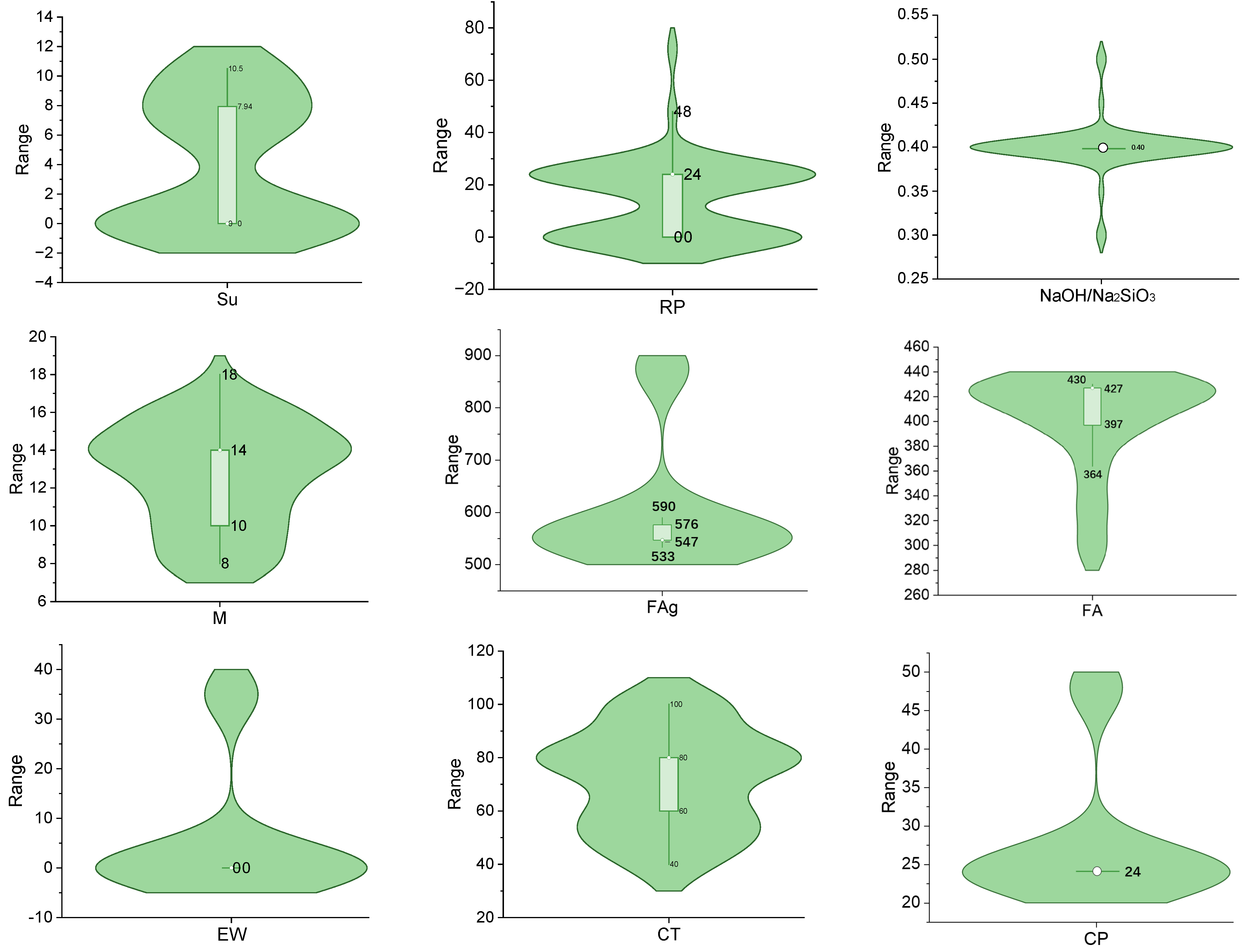
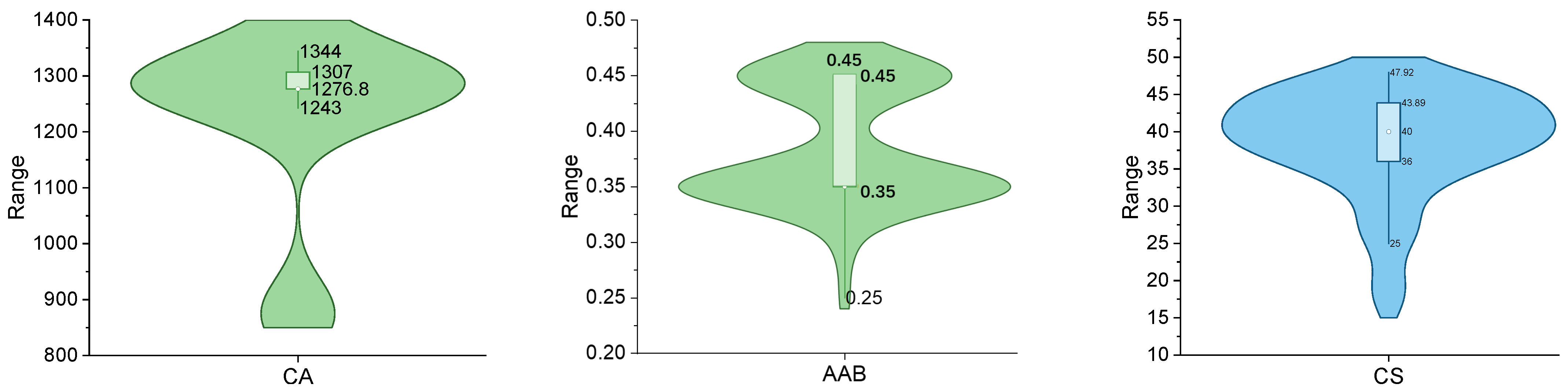
- Data Collection and Preprocessing: A dataset consisting of 63 observations of GeC was collected from a quarry mine in Malaysia. The dataset includes 11 input parameters, such as fly ash content, curing temperature, and alkaline activator ratio. These input features were normalized to the range [−1, 1] to ensure consistency in the model training process.
- 2.
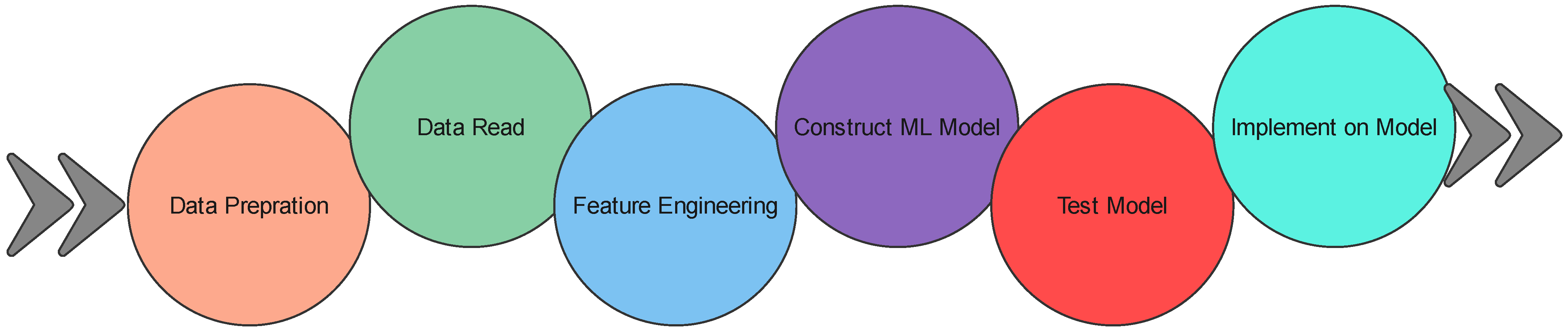
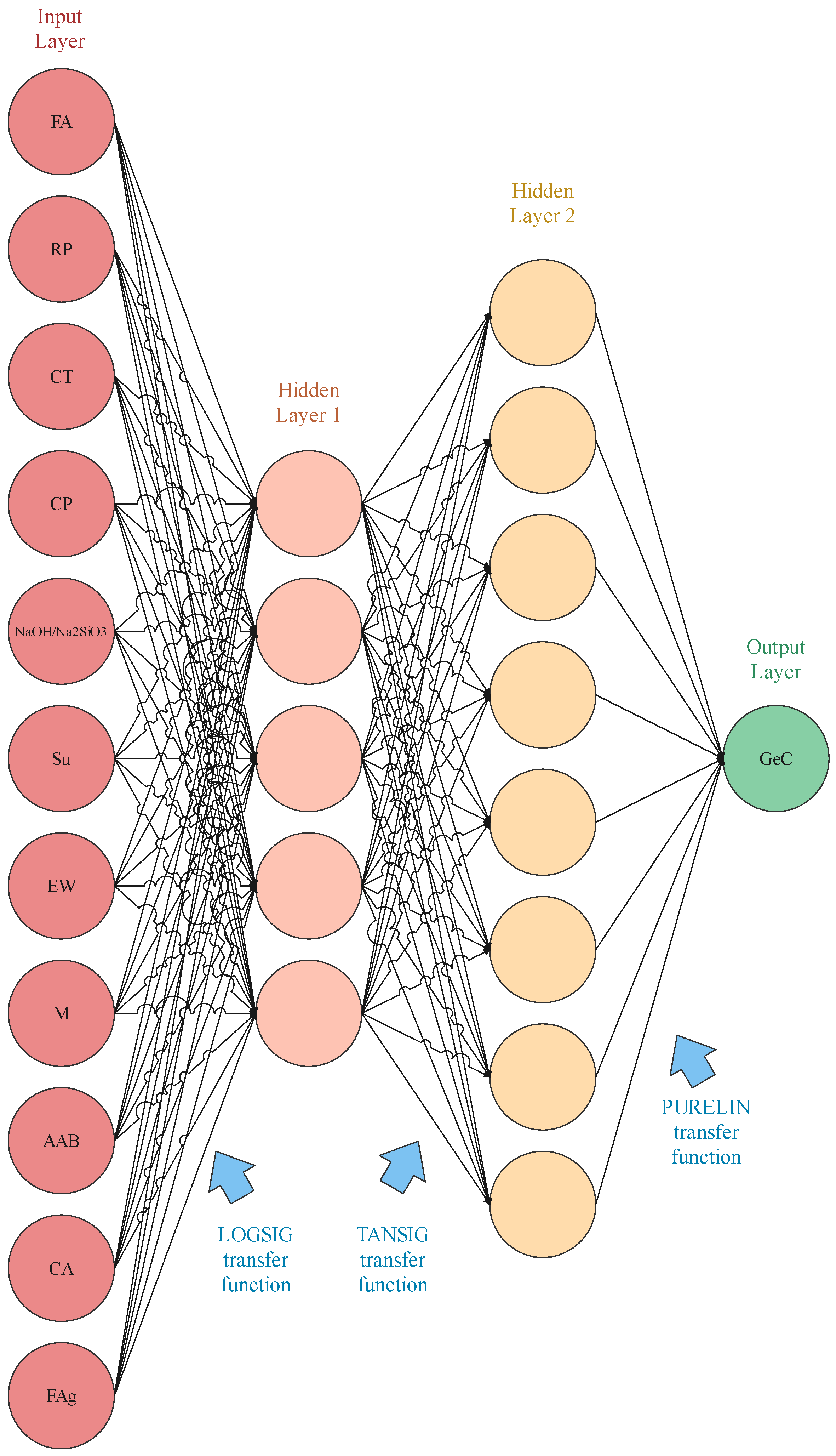
- Model Development: Three machine learning models were developed to predict the compressive strength of GeC:
- MLP Model: A basic neural network with varying numbers of hidden layers and neurons, trained using standard backpropagation.
- GOA–MLP Model: The MLP model optimized using the Gannet Optimization Algorithm (GOA) to tune the network’s hyperparameters.
- GWO–MLP Model: The MLP model optimized using the Grey Wolf Optimizer (GWO) to improve the model’s accuracy.
- 3.
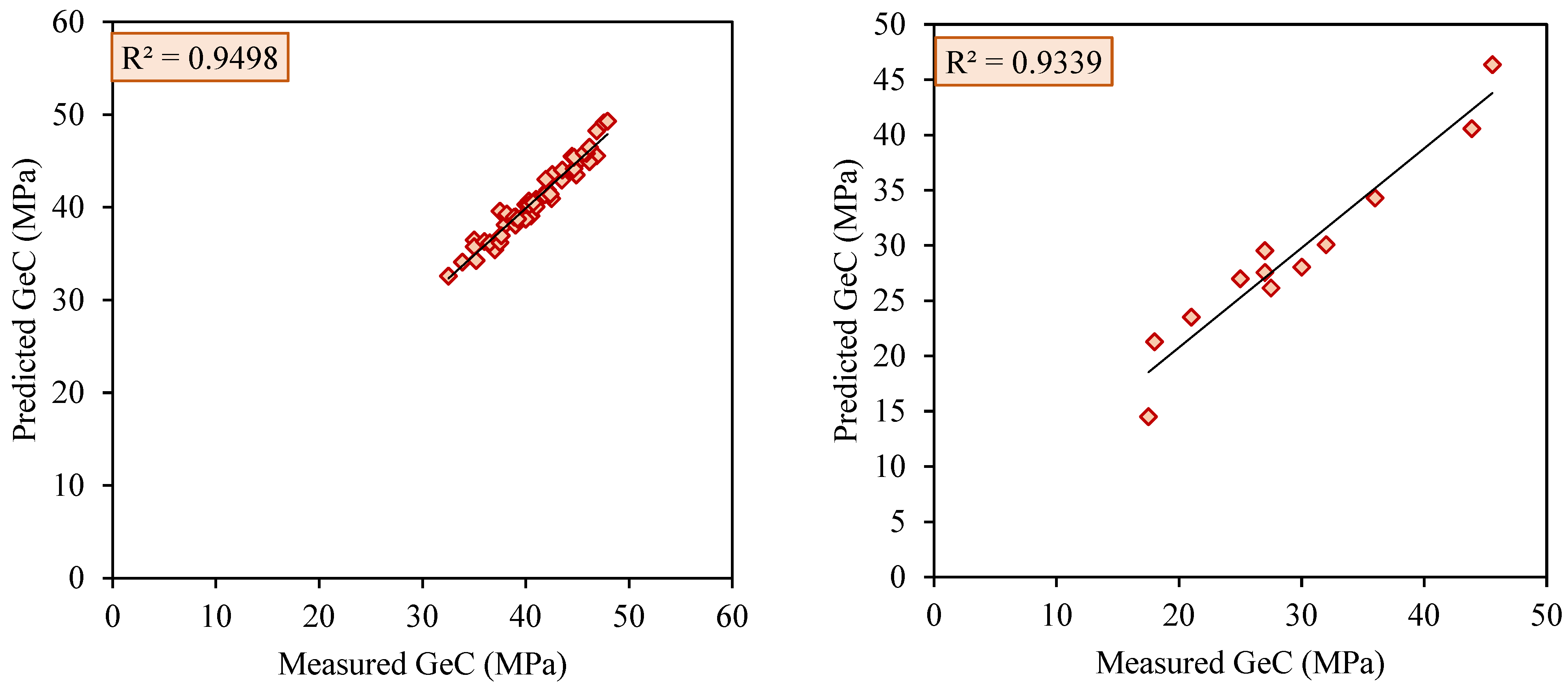
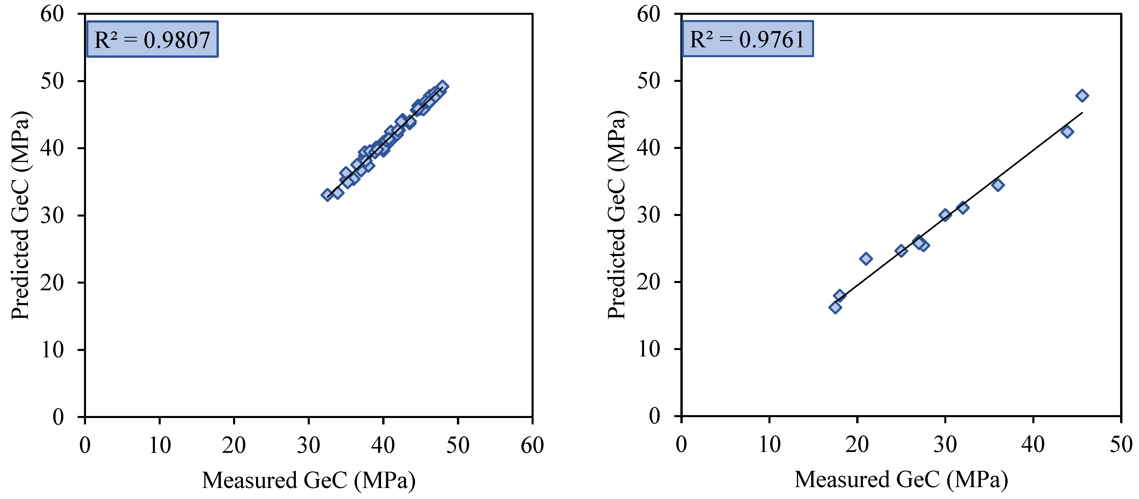
- Model Evaluation: The performance of each model was evaluated using R2, Root Mean Squared Error (RMSE), and Variance Accounted For (VAF) during both the training and testing phases. The models were trained on 80% of the data and tested on the remaining 20%. The hybrid models (GOA–MLP and GWO–MLP) were compared to the baseline MLP model to assess improvements in predictive accuracy.
- 4.
- Sensitivity Analysis: Sensitivity analysis was conducted to identify the key parameters influencing GeC’s compressive strength. This analysis helps to highlight the most critical factors that affect the material’s performance and provides insights into the optimal mix design for GeC.
- 5.
- Model Comparison and Discussion: The results were analyzed and compared to highlight the advantages of hybrid optimization algorithms (GOA and GWO) over the standard MLP model in improving prediction accuracy. The implications of the sensitivity analysis were also discussed to guide future research and practical applications of the models.
2.1. Research Techniques
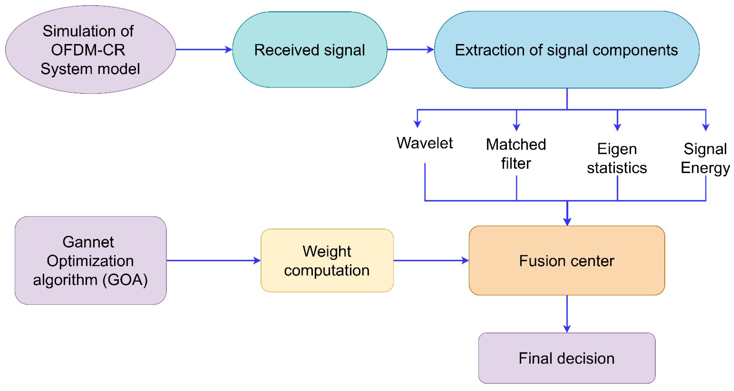
2.1.1. Gannet Optimization Algorithm (GOA)
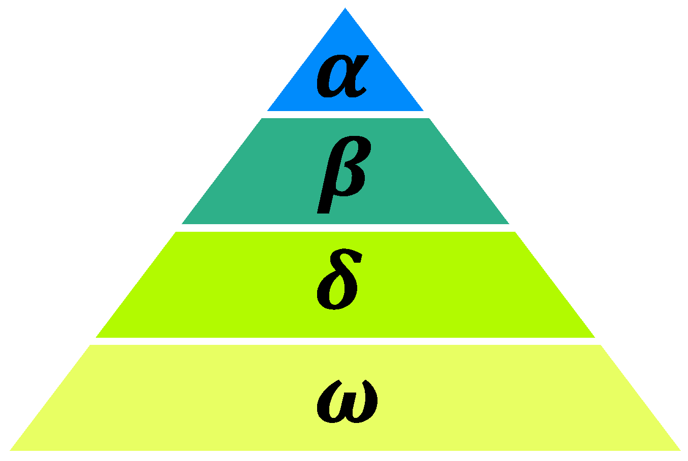
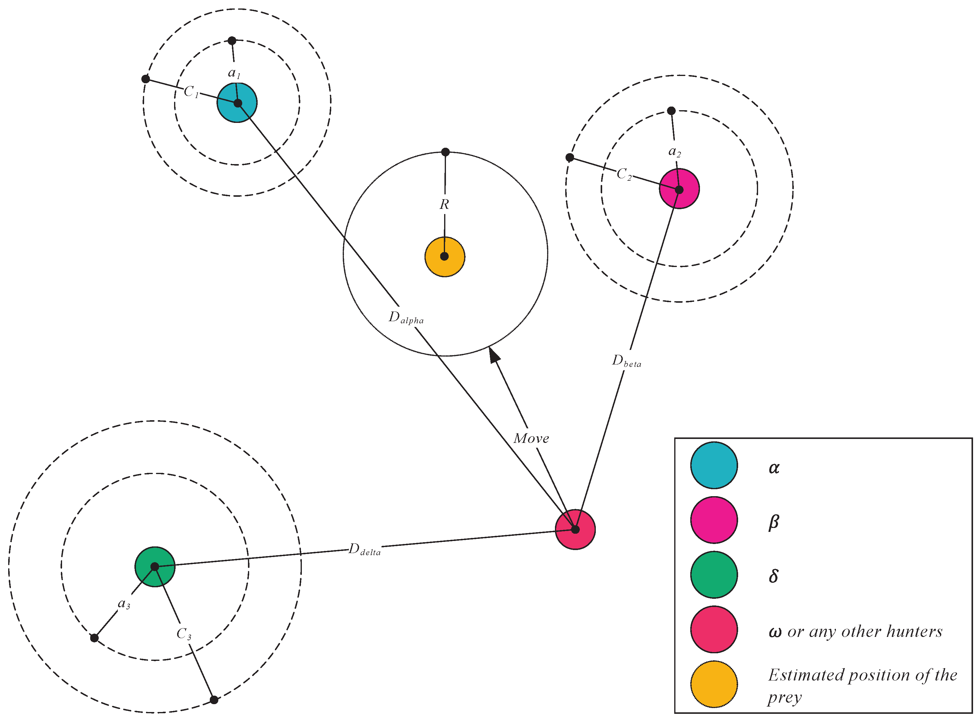
2.1.2. Grey Wolf Optimizer (GWO)
2.1.3. Artificial Neural Network
2.2. Case Study and Data Analysis
3. Model Development
3.1. MLP
3.2. Development of Hybrid Models
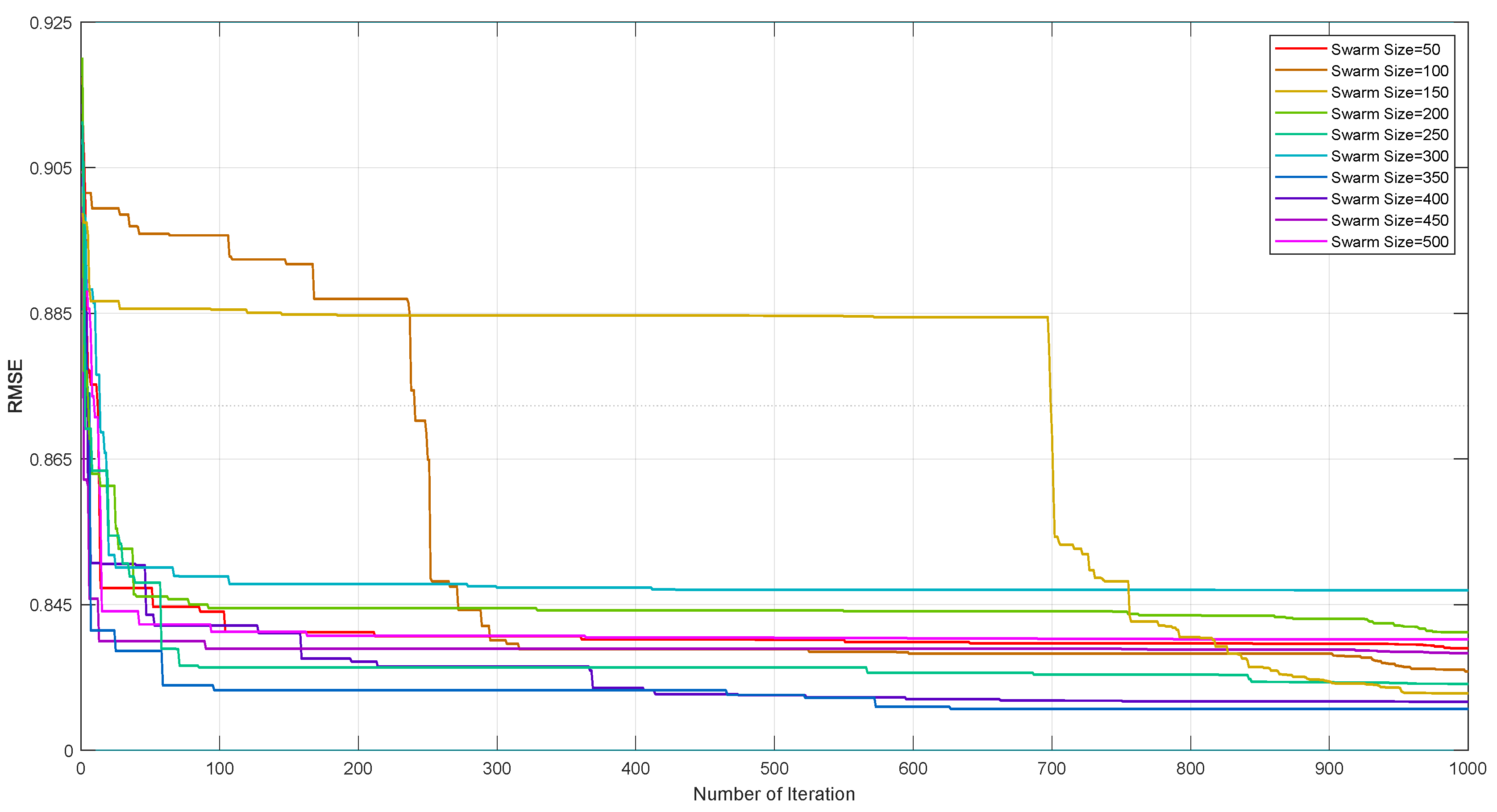
3.2.1. GOA–MLP
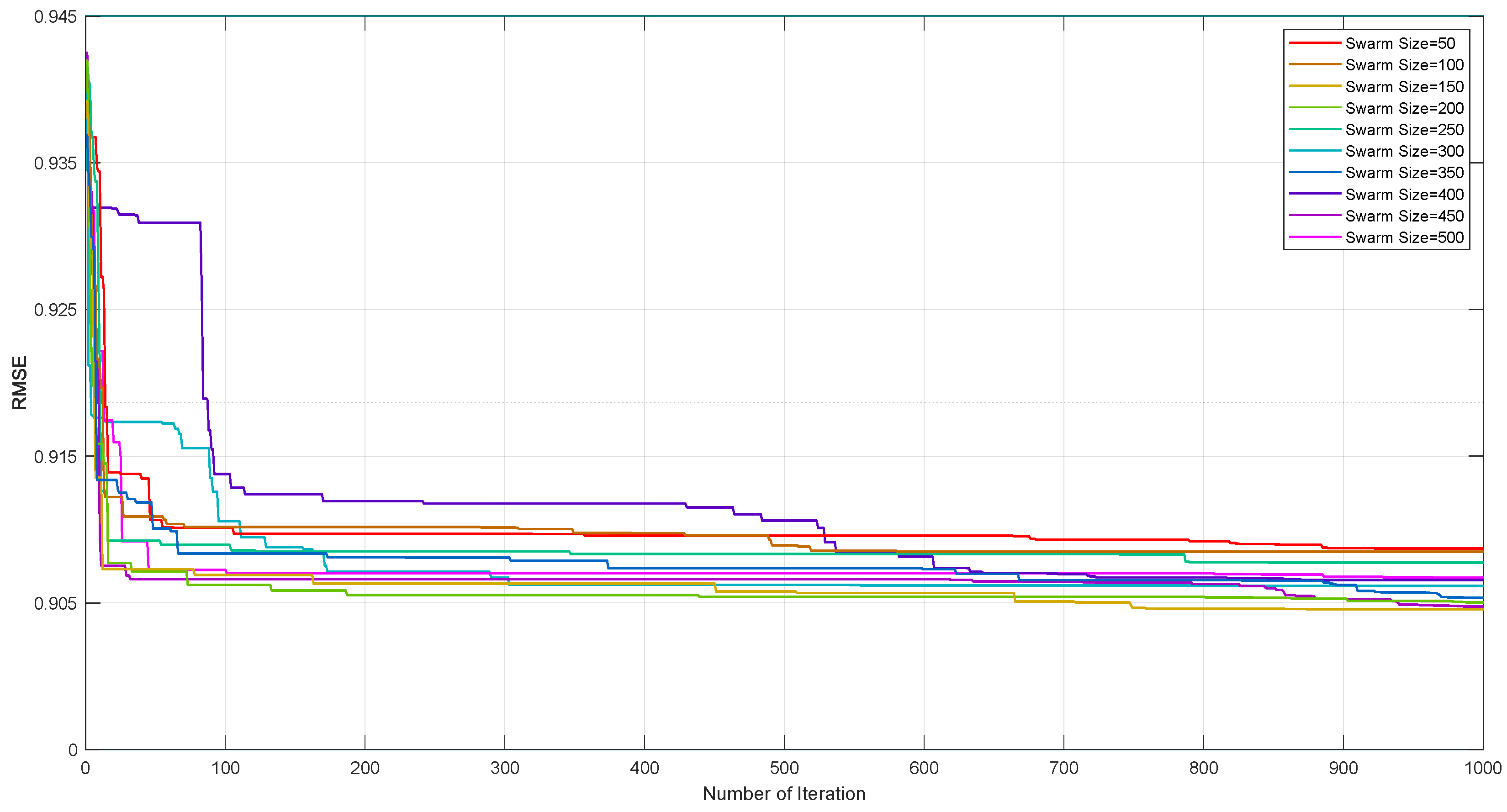
3.2.2. GWO–MLP
4. Results and Discussion
5. Sensitivity Analysis
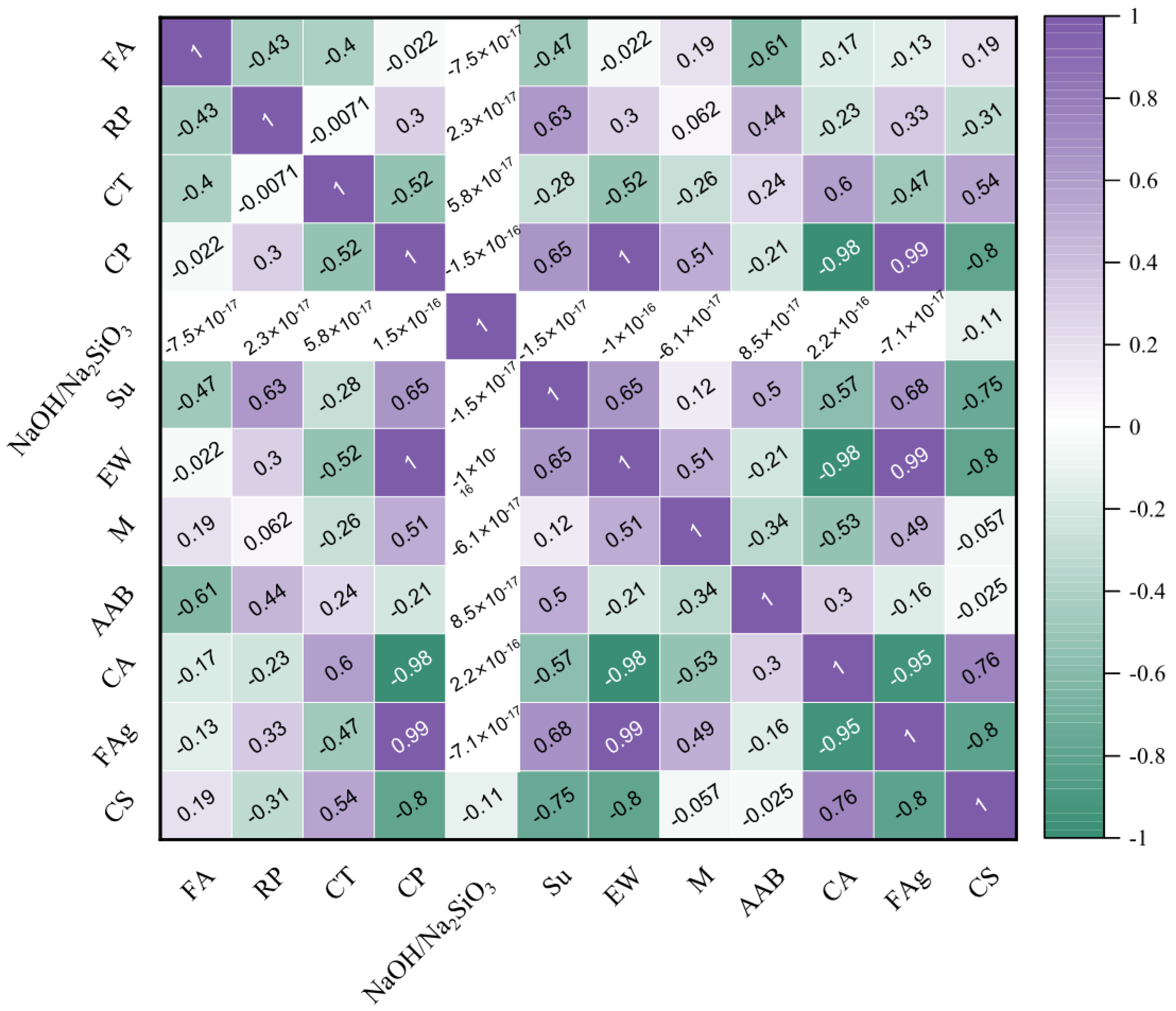
- CA: Ranked 1st, indicating that the calcium activator has the highest sensitivity and strongest influence on compressive strength. This suggests that variations in calcium activator content significantly affect concrete strength.
- FA: Ranked 2nd, showing a high sensitivity to changes in fly ash content. Fly ash is a crucial component in geopolymer concrete, influencing its mechanical properties.
- NaOH/Na2SiO3 Ratio: Ranked 3rd, indicating that the ratio of sodium hydroxide to sodium silicate affects compressive strength considerably. This ratio plays a vital role in geopolymerization reactions.
- CT: Ranked 4th, implying that curing temperature affects compressive strength but to a slightly lesser extent than the aforementioned parameters. Proper curing conditions are essential for achieving desired concrete strength.
- AAB: Ranked 5th, showing its significant but slightly lower impact compared to other parameters.
- M: Ranked 6th, indicating its moderate sensitivity to changes. Modulus of elasticity influences concrete’s ability to deform under stress.
- FAg: Ranked 7th, suggesting its sensitivity to compressive strength, albeit less than other parameters.
- CP: Ranked 8th, indicating that the duration of curing affects compressive strength, but it is relatively less influential compared to other factors.
- RP: Ranked 9th, implying that the presence and amount of reinforcement have a moderate impact on compressive strength.
- Su: Ranked 10th, suggesting its lower sensitivity compared to other parameters. Superplasticizers are used to improve workability but have a relatively minor effect on compressive strength.
- EW: Ranked 11th, indicating it has the least influence on compressive strength among the parameters analyzed.
6. Conclusions
Author Contributions
Funding
Data Availability Statement
Conflicts of Interest
References
- Jeyasehar, C.A.; Saravanan, G.; Salahuddin, M.; Thirugnanasambandam, S. Development of fly ash based geopolymer precast concrete elements. Asian J. Civ. Eng. 2013, 14, 605–615. [Google Scholar]
- Murthy, T.S.; Rai, D.A. Geopolymer Concrete, An Earth Friendly Concrete, Very Promising in the Industry. Int. J. Civ. Eng. Technol. 2014, 5, 113–122. [Google Scholar]
- CEA (Central Electricity Authority). Fly Ash Generation at Coal/Lignite Based Thermal Power Stations and Its Utilization in the Country Report; Central Electricity Authority: New Delhi, India, 2015. [Google Scholar]
- Kumar, R.; Dev, N. Effect of acids and freeze–thaw on the durability of modified rubberized concrete with optimum rubber crumb content. J. Appl. Polym. Sci. 2022, 139, 52191. [Google Scholar] [CrossRef]
- Verma, M.; Dev, N. Effect of ground granulated blast furnace slag and fly ash ratio and the curing conditions on the mechanical properties of geopolymer concrete. Struct. Concr. 2022, 23, 2015–2029. [Google Scholar] [CrossRef]
- Kumar, R.; Dev, N.; Ram, S.; Verma, M. Investigation of dry-wet cycles effect on the durability of modified rubberised concrete. Forces Mech. 2023, 10, 100168. [Google Scholar] [CrossRef]
- Borges, P.H.R.; Fonseca, L.F.; Nunes, V.A.; Panzera, T.H.; Martuscelli, C.C. Andreasen Particle Packing Method on the Development of Geopolymer Concrete for Civil Engineering. J. Mater. Civ. Eng. 2014, 26, 692–697. [Google Scholar] [CrossRef]
- Biondi, L.; Perry, M.; Vlachakis, C.; Wu, Z.; Hamilton, A.; McAlorum, J. Ambient cured fly ash geopolymer coatings for concrete. Materials 2019, 12, 923. [Google Scholar] [CrossRef] [PubMed]
- Gupta, A.; Gupta, N.; Saxena, K.K. Mechanical and durability characteristics assessment of geopolymer composite (gpc) at varying silica fume content. J. Compos. Sci. 2021, 5, 237. [Google Scholar] [CrossRef]
- Das, S.K.; Shrivastava, S. Siliceous fly ash and blast furnace slag based geopolymer concrete under ambient temperature curing condition. Struct. Concr. 2021, 22, E341–E351. [Google Scholar] [CrossRef]
- Zhou, J.; Su, Z.; Hosseini, S.; Tian, Q.; Lu, Y.; Luo, H.; Xu, X.; Chen, C.; Huang, J. Decision tree models for the estimation of geo-polymer concrete compressive strength. Math. Biosci. Eng. 2024, 21, 1413–1444. [Google Scholar] [CrossRef] [PubMed]
- Wang, Q.; Qi, J.; Hosseini, S.; Rasekh, H.; Huang, J. ICA-LightGBM Algorithm for Predicting Compressive Strength of Geo-Polymer Concrete. Buildings 2023, 13, 2278. [Google Scholar] [CrossRef]
- Indraratna, B.; Armaghani, D.J.; Correia, A.G.; Hunt, H.; Ngo, T. Prediction of resilient modulus of ballast under cyclic loading using machine learning techniques. Transp. Geotech. 2022, 38, 100895. [Google Scholar] [CrossRef]
- Medawela, S.; Armaghani, D.J.; Indraratna, B.; Rowe, R.K.; Thamwattana, N. Development of an advanced machine learning model to predict the pH of groundwater in permeable reactive barriers (PRBs) located in acidic terrain. Comput. Geotech. 2023, 161, 105557. [Google Scholar] [CrossRef]
- Armaghani, D.J.; Ming, Y.Y.; Mohammed, A.S.; Momeni, E.; Maizir, H. Effect of SVM Kernel Functions on Bearing Capacity Assessment of Deep Foundations. J. Soft Comput. Civ. Eng. 2023, 7, 111–128. [Google Scholar]
- Momeni, E.; He, B.; Abdi, Y.; Armaghani, D.J. Novel Hybrid XGBoost Model to Forecast Soil Shear Strength Based on Some Soil Index Tests. Comput. Model. Eng. Sci. 2023, 136, 2527–2550. [Google Scholar] [CrossRef]
- Zhou, J.; Wang, Z.; Li, C.; Wei, W.; Wang, S.; Armaghani, D.J.; Peng, K. Hybridized random forest with population-based optimization for predicting shear properties of rock fractures. J. Comput. Sci. 2023, 72, 102097. [Google Scholar] [CrossRef]
- Armaghani, D.J.; Asteris, P.G. A comparative study of ANN and ANFIS models for the prediction of cement-based mortar materials compressive strength. Neural Comput. Appl. 2021, 33, 4501–4532. [Google Scholar] [CrossRef]
- Skentou, A.D.; Bardhan, A.; Mamou, A.; Lemonis, M.E.; Kumar, G.; Samui, P.; Armaghani, D.J.; Asteris, P.G. Closed-Form Equation for Estimating Unconfined Compressive Strength of Granite from Three Non-destructive Tests Using Soft Computing Models. Rock Mech. Rock Eng. 2023, 56, 487–514. [Google Scholar] [CrossRef]
- Mahmood, W.; Mohammed, A.S.; Asteris, P.G.; Kurda, R.; Armaghani, D.J. Modeling Flexural and Compressive Strengths Behaviour of Cement-Grouted Sands Modified with Water Reducer Polymer. Appl. Sci. 2022, 12, 1016. [Google Scholar] [CrossRef]
- Asteris, P.G.; Lourenço, P.B.; Roussis, P.C.; Adami, C.E.; Armaghani, D.J.; Cavaleri, L.; Chalioris, C.E.; Hajihassani, M.; Lemonis, M.E.; Mohammed, A.S.; et al. Revealing the nature of metakaolin-based concrete materials using artificial intelligence techniques. Constr. Build. Mater. 2022, 322, 126500. [Google Scholar] [CrossRef]
- Barkhordari, M.S.; Armaghani, D.J.; Asteris, P.G. Structural Damage Identification Using Ensemble Deep Convolutional Neural Network Models. Comput. Model. Eng. Sci. 2022, 134, 835–855. [Google Scholar] [CrossRef]
- Cavaleri, L.; Barkhordari, M.S.; Repapis, C.C.; Armaghani, D.J.; Ulrikh, D.V.; Asteris, P.G. Convolution-based ensemble learning algorithms to estimate the bond strength of the corroded reinforced concrete. Constr. Build. Mater. 2022, 359, 129504. [Google Scholar] [CrossRef]
- Koopialipoor, M.; Asteris, P.G.; Mohammed, A.S.; Alexakis, D.E.; Mamou, A.; Armaghani, D.J. Introducing stacking machine learning approaches for the prediction of rock deformation. Transp. Geotech. 2022, 34, 100756. [Google Scholar] [CrossRef]
- Parsajoo, M.; Armaghani, D.J.; Mohammed, A.S.; Khari, M.; Jahandari, S. Tensile strength prediction of rock material using non-destructive tests: A comparative intelligent study. Transp. Geotech. 2021, 31, 100652. [Google Scholar] [CrossRef]
- Ahmad, A.; Ahmad, W.; Aslam, F.; Joyklad, P. Compressive strength prediction of fly ash-based geopolymer concrete via advanced machine learning techniques. Case Stud. Constr. Mater. 2022, 16, e00840. [Google Scholar] [CrossRef]
- Ahmad, A.; Chaiyasarn, K.; Farooq, F.; Ahmad, W.; Suparp, S.; Aslam, F. Compressive strength prediction via gene expression programming (Gep) and artificial neural network (ann) for concrete containing rca. Buildings 2021, 11, 324. [Google Scholar] [CrossRef]
- Song, H.; Ahmad, A.; Ostrowski, K.A.; Dudek, M. Analyzing the compressive strength of ceramic waste-based concrete using experiment and artificial neural network (Ann) approach. Materials 2021, 14, 4518. [Google Scholar] [CrossRef]
- Nguyen, H.; Vu, T.; Vo, T.P.; Thai, H.-T. Efficient machine learning models for prediction of concrete strengths. Constr. Build. Mater. 2021, 266, 120950. [Google Scholar] [CrossRef]
- Huang, J.; Sun, Y.; Zhang, J. Reduction of computational error by optimizing SVR kernel coefficients to simulate concrete compressive strength through the use of a human learning optimization algorithm. Eng. Comput. 2022, 38, 3151–3168. [Google Scholar] [CrossRef]
- Sarir, P.; Chen, J.; Asteris, P.G.; Armaghani, D.J.; Tahir, M.M. Developing GEP tree-based, neuro-swarm, and whale optimization models for evaluation of bearing capacity of concrete-filled steel tube columns. Eng. Comput. 2021, 37, 1–19. [Google Scholar] [CrossRef]
- Balf, F.R.; Kordkheili, H.M.; Kordkheili, A.M. A New Method for Predicting the Ingredients of Self-Compacting Concrete (SCC) Including Fly Ash (FA) Using Data Envelopment Analysis (DEA). Arab. J. Sci. Eng. 2021, 46, 4439–4460. [Google Scholar] [CrossRef]
- Ahmad, A.; Farooq, F.; Ostrowski, K.A.; Śliwa-Wieczorek, K.; Czarnecki, S. Application of novel machine learning techniques for predicting the surface chloride concentration in concrete containing waste material. Materials 2021, 14, 2297. [Google Scholar] [CrossRef] [PubMed]
- Azimi-Pour, M.; Eskandari-Naddaf, H.; Pakzad, A. Linear and non-linear SVM prediction for fresh properties and compressive strength of high volume fly ash self-compacting concrete. Constr. Build. Mater. 2020, 230, 117021. [Google Scholar] [CrossRef]
- Saha, P.; Debnath, P.; Thomas, P. Prediction of fresh and hardened properties of self-compacting concrete using support vector regression approach. Neural Comput. Appl. 2020, 32, 7995–8010. [Google Scholar] [CrossRef]
- Shahmansouri, A.A.; Bengar, H.A.; Jahani, E. Predicting compressive strength and electrical resistivity of eco-friendly concrete containing natural zeolite via GEP algorithm. Constr. Build. Mater. 2019, 229, 116883. [Google Scholar] [CrossRef]
- Aslam, F.; Farooq, F.; Amin, M.N.; Khan, K.; Waheed, A.; Akbar, A.; Javed, M.F.; Alyousef, R.; Alabdulijabbar, H. Applications of gene expression programming for estimating compressive strength of high-strength concrete. Adv. Civ. Eng. 2020, 2020, 8850535. [Google Scholar] [CrossRef]
- Farooq, F.; Amin, M.N.; Khan, K.; Sadiq, M.R.; Javed, M.F.; Aslam, F.; Alyousef, R. A comparative study of random forest and genetic engineering programming for the prediction of compressive strength of high strength concrete (HSC). Appl. Sci. 2020, 10, 7330. [Google Scholar] [CrossRef]
- Asteris, P.G.; Kolovos, K. Self-compacting concrete strength prediction using surrogate models. Neural Comput. Appl. 2019, 31, 409–424. [Google Scholar] [CrossRef]
- Huang, J.; Zhang, J.; Li, X.; Qiao, Y.; Zhang, R.; Kumar, G.S. Investigating the effects of ensemble and weight optimization approaches on neural networks’ performance to estimate the dynamic modulus of asphalt concrete. Road Mater. Pavement Des. 2023, 24, 1939–1959. [Google Scholar] [CrossRef]
- Zhang, J.; Ma, G.; Huang, Y.; Sun, J.; Aslani, F.; Nener, B. Modelling uniaxial compressive strength of lightweight self-compacting concrete using random forest regression. Constr. Build. Mater. 2019, 210, 713–719. [Google Scholar] [CrossRef]
- Kaveh, A.; Bakhshpoori, T.; Hamze-Ziabari, S.M. M5′ and mars based prediction models for properties of selfcompacting concrete containing fly ash. Period. Polytech. Civ. Eng. 2018, 62, 281–294. [Google Scholar] [CrossRef]
- Sathyan, D.; Anand, K.B.; Prakash, A.J.; Premjith, B. Modeling the Fresh and Hardened Stage Properties of Self-Compacting Concrete using Random Kitchen Sink Algorithm. Int. J. Concr. Struct. Mater. 2018, 12, 24. [Google Scholar] [CrossRef]
- Vakhshouri, B.; Nejadi, S. Prediction of compressive strength of self-compacting concrete by ANFIS models. Neurocomputing 2018, 280, 13–22. [Google Scholar] [CrossRef]
- Douma, O.B.; Boukhatem, B.; Ghrici, M.; Tagnit-Hamou, A. Prediction of properties of self-compacting concrete containing fly ash using artificial neural network. Neural Comput. Appl. 2017, 28, 707–718. [Google Scholar] [CrossRef]
- Abu Yaman, M.; Elaty, M.A.; Taman, M. Predicting the ingredients of self compacting concrete using artificial neural network. Alex. Eng. J. 2017, 56, 523–532. [Google Scholar] [CrossRef]
- Ahmad, A.; Farooq, F.; Niewiadomski, P.; Ostrowski, K.; Akbar, A.; Aslam, F.; Alyousef, R. Prediction of compressive strength of fly ash based concrete using individual and ensemble algorithm. Materials 2021, 14, 794. [Google Scholar] [CrossRef]
- Farooq, F.; Ahmed, W.; Akbar, A.; Aslam, F.; Alyousef, R. Predictive modeling for sustainable high-performance concrete from industrial wastes: A comparison and optimization of models using ensemble learners. J. Clean. Prod. 2021, 292, 126032. [Google Scholar] [CrossRef]
- Bušić, R. Prediction Models for the Mechanical Properties of Self-Compacting Concrete with Recycled Rubber and Silica Fume. Materials 2020, 13, 1821. [Google Scholar] [CrossRef] [PubMed]
- Javed, M.F.; Farooq, F.; Memon, S.A.; Akbar, A.; Khan, M.A.; Aslam, F.; Alyousef, R.; Alabduljabbar, H.; Rehman, S.K.U.; Rehman, S.K.U.; et al. New prediction model for the ultimate axial capacity of concrete-filled steel tubes: An evolutionary approach. Crystals 2020, 10, 741. [Google Scholar] [CrossRef]
- Nematzadeh, M.; Shahmansouri, A.A.; Fakoor, M. Post-fire compressive strength of recycled PET aggregate concrete reinforced with steel fibers: Optimization and prediction via RSM and GEP. Constr. Build. Mater. 2020, 252, 119057. [Google Scholar] [CrossRef]
- Verma, M.; Nigam, M. Mechanical Behaviour of Self Compacting and Self Curing Concrete. Int. J. Innov. Res. Sci. Eng. Technol. 2017, 6, 14361–14366. [Google Scholar] [CrossRef]
- Verma, M.; Dev, N. Sodium hydroxide effect on the mechanical properties of flyash-slag based geopolymer concrete. Struct. Concr. 2021, 22, E368–E379. [Google Scholar] [CrossRef]
- Chouksey, A.; Verma, M.; Dev, N.; Rahman, I.; Upreti, K. An investigation on the effect of curing conditions on the mechanical and microstructural properties of the geopolymer concrete. Mater. Res. Express 2022, 9, 055003. [Google Scholar] [CrossRef]
- Reddy, K.C. Investigation of Mechanical and Microstructural Properties of Fiber-Reinforced Geopolymer Concrete with GGBFS and Metakaolin: Novel Raw Material for Geopolymerisation. Silicon 2021, 13, 4565–4573. [Google Scholar] [CrossRef]
- Hasanipanah, M.; Monjezi, M.; Shahnazar, A.; Jahed Armaghani, D.; Farazmand, A. Feasibility of indirect determination of blast induced ground vibration based on support vector machine. Meas. J. Int. Meas. Confed. 2015, 75, 289–297. [Google Scholar] [CrossRef]
- Momeni, E.; Nazir, R.; Armaghani, D.J.; Maizir, H. Prediction of pile bearing capacity using a hybrid genetic algorithm-based ANN. Measurement 2014, 57, 122–131. [Google Scholar] [CrossRef]
- He, B.; Armaghani, D.J.; Lai, S.H. Assessment of tunnel blasting-induced overbreak: A novel metaheuristic-based random forest approach. Tunn. Undergr. Space Technol. 2023, 133, 104979. [Google Scholar] [CrossRef]
- Li, D.; Liu, Z.; Armaghani, D.J.; Xiao, P.; Zhou, J. Novel Ensemble Tree Solution for Rockburst Prediction Using Deep Forest. Mathematics 2022, 10, 787. [Google Scholar] [CrossRef]
- Asteris, P.G.; Rizal, F.I.M.; Koopialipoor, M.; Roussis, P.C.; Ferentinou, M.; Armaghani, D.J.; Gordan, B. Slope Stability Classification under Seismic Conditions Using Several Tree-Based Intelligent Techniques. Appl. Sci. 2022, 12, 1753. [Google Scholar] [CrossRef]
- Zhou, J.; Huang, S.; Zhou, T.; Armaghani, D.J.; Qiu, Y. Employing a genetic algorithm and grey wolf optimizer for optimizing RF models to evaluate soil liquefaction potential. Artif. Intell. Rev. 2022, 55, 5673–5705. [Google Scholar] [CrossRef]
- Xie, C.; Nguyen, H.; Choi, Y.; Armaghani, D.J. Optimized functional linked neural network for predicting diaphragm wall deflection induced by braced excavations in clays. Geosci. Front. 2022, 13, 101313. [Google Scholar] [CrossRef]
- Zhou, J.; Qiu, Y.; Zhu, S.; Armaghani, D.J.; Khandelwal, M.; Mohamad, E.T. Estimation of the TBM advance rate under hard rock conditions using XGBoost and Bayesian optimization. Undergr. Space 2021, 6, 506–515. [Google Scholar] [CrossRef]
- Zhou, J.; Qiu, Y.; Zhu, S.; Armaghani, D.J.; Li, C.; Nguyen, H.; Yagiz, S. Optimization of support vector machine through the use of metaheuristic algorithms in forecasting TBM advance rate. Eng. Appl. Artif. Intell. 2021, 97, 104015. [Google Scholar] [CrossRef]
- Armaghani, D.J.; Koopialipoor, M.; Marto, A.; Yagiz, S. Application of several optimization techniques for estimating TBM advance rate in granitic rocks. J. Rock Mech. Geotech. Eng. 2019, 11, 779–789. [Google Scholar] [CrossRef]
- Jiskani, I.M.; Yasli, F.; Hosseini, S.; Rehman, A.U.; Uddin, S. Improved Z-number based fuzzy fault tree approach to analyze health and safety risks in surface mines. Resour. Policy 2022, 76, 102591. [Google Scholar] [CrossRef]
- Poormirzaee, R.; Hosseini, S.; Taghizadeh, R. Smart mining policy: Integrating fuzzy-VIKOR technique and the Z-number concept to implement industry 4.0 strategies in mining engineering. Resour. Policy 2022, 77, 102768. [Google Scholar] [CrossRef]
- Hosseini, S.; Lawal, A.I.; Kwon, S. A causality-weighted approach for prioritizing mining 4.0 strategies integrating reliability-based fuzzy cognitive map and hybrid decision-making methods: A case study of Nigerian Mining Sector. Resour. Policy 2023, 82, 103426. [Google Scholar] [CrossRef]
- Mikaeil, R.; Bakhtavar, E.; Hosseini, S.; Jafarpour, A. Fuzzy classification of rock engineering indices using rock texture characteristics. Bull. Eng. Geol. Environ. 2022, 81, 312. [Google Scholar] [CrossRef]
- Poormirzaee, R.; Hosseini, S.S.; Taghizadeh, R. Choosing the Appropriate Strategy of 4.0 Industries for the Implementation of Intelligent Methods in Mining Engineering. J. Miner. Resour. Eng. 2023, 8, 71–93. [Google Scholar]
- Hosseini, S.S.; Poormirzaee, R.; Moosazadeh, S. Study of Hazards in Underground Mining: Using Fuzzy Cognitive Map and Z-Number Theory for Prioritizing of effective Factors on Occupational Hazards in Underground Mines. J. Min. Eng. 2022, 17, 11–20. [Google Scholar]
- Kaveh, A.; Khalegi, A. Prediction of Strength for Concrete Specimens using Artificial Neural Networks. In Advances in Engineering Computational Technology; Civil-Comp Press: Edinburgh, UK, 1998. [Google Scholar] [CrossRef]
- Pan, J.-S.; Zhang, L.-G.; Wang, R.-B.; Snášel, V.; Chu, S.-C. Gannet optimization algorithm: A new metaheuristic algorithm for solving engineering optimization problems. Math. Comput. Simul. 2022, 202, 343–373. [Google Scholar] [CrossRef]
- Alkahtani, M.; Abidi, M.H.; Bin Obaid, H.S.; Alotaik, O. Modified gannet optimization algorithm for reducing system operation cost in engine parts industry with pooling management and transport optimization. Sustainability 2023, 15, 13815. [Google Scholar] [CrossRef]
- Rao, D.R.; Prasad, T.J.; Prasad, M.N.G. Gannet optimization algorithm enabled framework for spectrum sensing in OFDM based CR network. Wirel. Netw. 2023, 29, 2863–2872. [Google Scholar] [CrossRef]
- Yanzhen, X.; Donghui, W. An improved grey wolf optimization algorithm based on convergence factor. Netw. New Media Technol. 2020, 9, 28–34. [Google Scholar]
- Wu, Z.; Zhao, X.; Fan, D. Research on the Influence of Traction Load on Transient Stability of Power Grid Based on Parameter Identification. Energies 2023, 16, 7553. [Google Scholar] [CrossRef]
- Feng, J.; Sun, C.; Zhang, J.; Du, Y.; Liu, Z.; Ding, Y. A UAV Path Planning Method in Three-Dimensional Space Based on a Hybrid Gray Wolf Optimization Algorithm. Electronics 2023, 13, 68. [Google Scholar] [CrossRef]
- Mirjalili, S.; Mirjalili, S.M.; Lewis, A. Grey Wolf Optimizer. Adv. Eng. Softw. 2014, 69, 46–61. [Google Scholar] [CrossRef]
- Esangbedo, M.O.; Taiwo, B.O.; Abbas, H.H.; Hosseini, S.; Sazid, M.; Fissha, Y. Enhancing the exploitation of natural resources for green energy: An application of LSTM-based meta-model for aluminum prices forecasting. Resour. Policy 2024, 92, 105014. [Google Scholar] [CrossRef]
- Verma, M. Prediction of compressive strength of geopolymer concrete using random forest machine and deep learning. Asian J. Civ. Eng. 2023, 24, 2659–2668. [Google Scholar] [CrossRef]
- Hosseini, S.; Entezam, S.; Shokri, B.J.; Mirzaghorbanali, A.; Nourizadeh, H.; Motallebiyan, A.; Entezam, A.; McDougall, K.; Karunasena, W.; Aziz, N. Predicting grout’s uniaxial compressive strength (UCS) for fully grouted rock bolting system by applying ensemble machine learning techniques. Neural Comput. Appl. 2024, 36, 18387–18412. [Google Scholar] [CrossRef]
- Shokri, B.J.; Mirzaghorbanali, A.; McDougall, K.; Karunasena, W.; Nourizadeh, H.; Entezam, S.; Hosseini, S.; Aziz, N. Data-Driven Optimised XGBoost for Predicting the Performance of Axial Load Bearing Capacity of Fully Cementitious Grouted Rock Bolting Systems. Appl. Sci. 2024, 14, 9925. [Google Scholar] [CrossRef]
- Bin, F.; Hosseini, S.; Chen, J.; Samui, P.; Fattahi, H.; Armaghani, D.J. Proposing Optimized Random Forest Models for Predicting Compressive Strength of Geopolymer Composites. Infrastructures 2024, 9, 181. [Google Scholar] [CrossRef]
- Akber, M.Z.; Chan, W.-K.; Lee, H.-H.; Anwar, G.A. TPE-Optimized DNN with Attention Mechanism for Prediction of Tower Crane Payload Moving Conditions. Mathematics 2024, 12, 3006. [Google Scholar] [CrossRef]
- Hosseini, S.; Khatti, J.; Taiwo, B.O.; Fissha, Y.; Grover, K.S.; Ikeda, H.; Pushkarna, M.; Berhanu, M.; Ali, M. Assessment of the ground vibration during blasting in mining projects using different computational approaches. Sci. Rep. 2023, 13, 18582. [Google Scholar] [CrossRef] [PubMed]
- Hosseini, S.; Poormirzaee, R.; Gilani, S.-O.; Jiskani, I.M. A reliability-based rock engineering system for clean blasting: Risk analysis and dust emissions forecasting. Clean Technol. Environ. Policy 2023, 25, 1903–1920. [Google Scholar] [CrossRef]
- Taiwo, B.O.; Hosseini, S.; Fissha, Y.; Kilic, K.; Olusola, O.A.; Chandrahas, N.S.; Li, E.; Akinlabi, A.A.; Khan, N.M. Indirect Evaluation of the Influence of Rock Boulders in Blasting to the Geohazard: Unearthing Geologic Insights Fused with Tree Seed based LSTM Algorithm. Geohazard Mech. 2024, in press. [Google Scholar] [CrossRef]
- Hosseini, S.; Pourmirzaee, R.; Armaghani, D.J.; Sabri, M.M.S. Prediction of ground vibration due to mine blasting in a surface lead–zinc mine using machine learning ensemble techniques. Sci. Rep. 2023, 13, 6591. [Google Scholar] [CrossRef] [PubMed]
- Hosseini, S.; Mousavi, A.; Monjezi, M.; Khandelwal, M. Mine-to-crusher policy: Planning of mine blasting patterns for environmentally friendly and optimum fragmentation using Monte Carlo simulation-based multi-objective grey wolf optimization approach. Resour. Policy 2022, 79, 103087. [Google Scholar] [CrossRef]
- Hosseini, S.; Monjezi, M.; Bakhtavar, E. Minimization of blast-induced dust emission using gene-expression programming and grasshopper optimization algorithm: A smart mining solution based on blasting plan optimization. Clean Technol. Environ. Policy 2022, 24, 2313–2328. [Google Scholar] [CrossRef]
- Hosseini, S.; Monjezi, M.; Bakhtavar, E.; Mousavi, A. Prediction of Dust Emission Due to Open Pit Mine Blasting Using a Hybrid Artificial Neural Network. Nat. Resour. Res. 2021, 30, 4773–4788. [Google Scholar] [CrossRef]
- Bakhtavar, E.; Hosseini, S.; Hewage, K.; Sadiq, R. Air Pollution Risk Assessment Using a Hybrid Fuzzy Intelligent Probability-Based Approach: Mine Blasting Dust Impacts. Nat. Resour. Res. 2021, 30, 2607–2627. [Google Scholar] [CrossRef]
- Bakhtavar, E.; Hosseini, S.; Hewage, K.; Sadiq, R. Green blasting policy: Simultaneous forecast of vertical and horizontal distribution of dust emissions using artificial causality-weighted neural network. J. Clean. Prod. 2021, 283, 124562. [Google Scholar] [CrossRef]
- Taiwo, B.O.; Fissha, Y.; Hosseini, S.; Khishe, M.; Kahraman, E.; Adebayo, B.; Sazid, M.; Adesida, P.A.; Famobuwa, O.V.; Faluyi, J.O.; et al. Machine learning based prediction of flyrock distance in rock blasting: A safe and sustainable mining approach. Green Smart Min. Eng. 2024, 1, 346–361. [Google Scholar] [CrossRef]
- Hosseini, S.; Shokri, B.J.; Mirzaghorbanali, A.; Nourizadeh, H.; Entezam, S.; Motallebiyan, A.; Entezam, A.; McDougall, K.; Karunasena, W.; Aziz, N. Predicting axial-bearing capacity of fully grouted rock bolting systems by applying an ensemble system. Soft Comput. 2024, 28, 10491–10518. [Google Scholar] [CrossRef]
- Hosseini, S.; Poormirzaee, R.; Hajihassani, M. An uncertainty hybrid model for risk assessment and prediction of blast-induced rock mass fragmentation. Int. J. Rock Mech. Min. Sci. 2022, 160, 105250. [Google Scholar] [CrossRef]
- Kamran, M.; Chaudhry, W.; Taiwo, B.O.; Hosseini, S.; Rehman, H. Decision intelligence-based predictive modelling of hard rock pillar stability using k-nearest neighbour coupled with grey wolf optimization algorithm. Processes 2024, 12, 783. [Google Scholar] [CrossRef]
- Wang, X.; Hosseini, S.; Armaghani, D.J.; Mohamad, E.T. Data-Driven Optimized Artificial Neural Network Technique for Prediction of Flyrock Induced by Boulder Blasting. Mathematics 2023, 11, 2358. [Google Scholar] [CrossRef]
- Hosseini, S.; Gordan, B.; Kalkan, E. Development of Z number-based fuzzy inference system to predict bearing capacity of circular foundations. Artif. Intell. Rev. 2024, 57, 146. [Google Scholar] [CrossRef]
- Hosseini, S.; Mousavi, A.; Monjezi, M. Prediction of blast-induced dust emissions in surface mines using integration of dimensional analysis and multivariate regression analysis. Arab. J. Geosci. 2022, 15, 163. [Google Scholar] [CrossRef]
- Hosseini, S.; Poormirzaee, R.; Hajihassani, M. Application of reliability-based back-propagation causality-weighted neural networks to estimate air-overpressure due to mine blasting. Eng. Appl. Artif. Intell. 2022, 115, 105281. [Google Scholar] [CrossRef]
- Hosseini, S.; Poormirzaee, R.; Hajihassani, M.; Kalatehjari, R. An ANN-Fuzzy Cognitive Map-Based Z-Number Theory to Predict Flyrock Induced by Blasting in Open-Pit Mines. Rock Mech. Rock Eng. 2022, 55, 4373–4390. [Google Scholar] [CrossRef]
- Lawal, A.I.; Hosseini, S.; Kim, M.; Ogunsola, N.O.; Kwon, S. Prediction of factor of safety of slopes using stochastically modified ANN and classical methods: A rigorous statistical model selection approach. Nat. Hazards 2023, 120, 2035–2056. [Google Scholar] [CrossRef]
- Pourmirzaee, R.; Hosseini, S. Development of an ANN-Based Technique for Inversion of Seismic Refraction Travel Times. J. Environ. Eng. Geophys. 2024, 29, 75–90. [Google Scholar] [CrossRef]
- Zhang, Z.; Hosseini, S.; Monjezi, M.; Yari, M. Extension of reliability information of Z-numbers and fuzzy cognitive map: Development of causality-weighted rock engineering system to predict and risk assessment of blast-induced rock size distribution. Int. J. Rock Mech. Min. Sci. 2024, 178, 105779. [Google Scholar] [CrossRef]
- Hosseini, S.; Javanshir, S.; Sabeti, H.; Tahmasebizadeh, P. Mathematical-Based Gene Expression Programming (GEP): A Novel Model to Predict Zinc Separation from a Bench-Scale Bioleaching Process. J. Sustain. Met. 2023, 9, 1601–1619. [Google Scholar] [CrossRef]
- Hosseini, S.; Pourmirzaee, R. Green Policy for Managing Blasting Induced Dust Dispersion in Open-pit Mines Using Probability-based Deep Learning Algorithm. Expert Syst. Appl. 2023, 240, 122469. [Google Scholar] [CrossRef]
- Kahraman, E.; Hosseini, S.; Taiwo, B.O.; Fissha, Y.; Jebutu, V.A.; Akinlabi, A.A.; Adachi, T. Fostering Sustainable Mining Practices in Rock Blasting: Assessment of Blast Toe Volume Prediction using Comparative Analysis of Hybrid Ensemble Machine Learning Techniques. J. Saf. Sustain. 2024, 1, 75–88. [Google Scholar] [CrossRef]
- Bolón-Canedo, V.; Remeseiro, B. Feature selection in image analysis: A survey. Artif. Intell. Rev. 2020, 53, 2905–2931. [Google Scholar] [CrossRef]
- Kabir, H.; Garg, N. Machine learning enabled orthogonal camera goniometry for accurate and robust contact angle measurements. Sci. Rep. 2023, 13, 1497. [Google Scholar] [CrossRef]
- Yang, Y.; Zhang, Q. A hierarchical analysis for rock engineering using artificial neural networks. Rock Mech. Rock Eng. 1997, 30, 207–222. [Google Scholar] [CrossRef]
- Zhao, J.; Hosseini, S.; Chen, Q.; Armaghani, D.J. Super learner ensemble model: A novel approach for predicting monthly copper price in future. Resour. Policy 2023, 85, 103903. [Google Scholar] [CrossRef]


| Author | Year | Technique | Number of Data |
|---|---|---|---|
| Huang et al. [30] | 2021 | SVM | 114 |
| Sarir et al. [31] | 2019 | GEP | 303 |
| Balf et al. [32] | 2021 | DEA | 114 |
| Ahmad et al. [33] | 2021 | GEP, ANN, DT | 642 |
| Azimi-Pour et al. [34] | 2020 | SVM | - |
| Saha et al. [35] | 2020 | SVM | 115 |
| Hahmansouri et al. [36] | 2020 | GEP | 351 |
| Hahmansouri et al. [36] | 2019 | GEP | 54 |
| Aslam et al. [37] | 2020 | GEP | 357 |
| Farooq et al. [38] | 2020 | RF and GEP | 357 |
| Asteris and Kolovos [39] | 2019 | ANN | 205 |
| Huang et al. [40] | 2019 | IREMSVM-FR withRSM | 114 |
| Zhang et al. [41] | 2019 | RF | 131 |
| Kaveh et al. [42] | 2018 | M5MARS | 114 |
| Sathyan et al. [43] | 2018 | RKSA | 40 |
| Vakhshouri and Nejadi [44] | 2018 | ANFIS | 55 |
| Belalia Douma et al. [45] | 2017 | ANN | 114 |
| Abu Yaman et al. [46] | 2017 | ANN | 69 |
| Ahmad et al. [47] | 2021 | GEP, DT and Bagging | 270 |
| Farooq et al. [48] | 2021 | ANN, bagging and boosting | 1030 |
| Bušić et al. [49] | 2020 | MV | 21 |
| Javad et al. [50] | 2020 | GEP | 277 |
| Nematzadeh et al. [51] | 2020 | RSM, GEP | 108 |
| Parameter | Symbol | Unit | Minimum | Average | Maximum | StD | |
|---|---|---|---|---|---|---|---|
| 1 | Fly ash | FA | (kg/m3) | 298.000 | 401.918 | 430.000 | 39.127 |
| 2 | Restperiod | RP | (hr) | 0.000 | 14.164 | 72.000 | 14.780 |
| 3 | Curingtemperature | CT | (°C) | 40.000 | 71.803 | 100.000 | 18.664 |
| 4 | Curingperiod | CP | (hr) | 24.000 | 27.934 | 48.000 | 8.959 |
| 5 | NaOH/Na2SiO3 | NaOH/Na2SiO3 | - | 0.300 | 0.400 | 0.500 | 0.027 |
| 6 | Superplasticizer | Su | (kg/m3) | 0.000 | 4.108 | 10.500 | 4.379 |
| 7 | Extrawater added | EW | (kg/m3) | 0.000 | 5.738 | 35.000 | 13.065 |
| 8 | Molarity | M | - | 8.000 | 12.656 | 18.000 | 2.774 |
| 9 | Alkalineactivator/binder ratio | AAB | - | 0.250 | 0.384 | 0.450 | 0.053 |
| 10 | Coarseaggregate | CA | (kg/m3) | 875.000 | 1223.915 | 1377.000 | 158.900 |
| 11 | Fineaggregate | FAg | (kg/m3) | 533.000 | 605.557 | 875.000 | 121.045 |
| 12 | Compressive strength | GeC | (MPa) | 17.500 | 38.713 | 47.920 | 7.077 |
| Model No. | Training | Testing | Training Rates | Testing Rates | Total Rate | Rank | ||||||||
|---|---|---|---|---|---|---|---|---|---|---|---|---|---|---|
| R2 | RMSE | VAF | R2 | RMSE | VAF | R2 | RMSE | VAF | R2 | RMSE | VAF | |||
| 1 | 0.929 | 10.941 | 92.483 | 0.9123 | 11.569 | 59.771 | 4 | 3 | 8 | 7 | 3 | 3 | 28 | 7 |
| 2 | 0.9486 | 7.255 | 83.183 | 0.8756 | 8.861 | 59.732 | 9 | 9 | 5 | 3 | 9 | 2 | 37 | 4 |
| 3 | 0.898 | 13.496 | 64.683 | 0.8671 | 13.086 | 54.826 | 1 | 1 | 1 | 2 | 1 | 1 | 7 | 10 |
| 4 | 0.9498 | 6.132 | 97.71 | 0.9339 | 8.863 | 94.961 | 10 | 10 | 10 | 10 | 8 | 10 | 58 | 1 |
| 5 | 0.9365 | 10.944 | 72.489 | 0.8643 | 9.547 | 65.395 | 7 | 2 | 2 | 1 | 6 | 5 | 23 | 9 |
| 6 | 0.9094 | 10.692 | 82.858 | 0.8951 | 10.743 | 64.812 | 2 | 5 | 4 | 6 | 4 | 4 | 25 | 8 |
| 7 | 0.9196 | 10.705 | 87.583 | 0.8785 | 10.445 | 75.625 | 3 | 4 | 7 | 4 | 5 | 8 | 31 | 5 |
| 8 | 0.9344 | 8.569 | 95.339 | 0.9171 | 9.491 | 75.572 | 6 | 8 | 9 | 8 | 7 | 7 | 45 | 3 |
| 9 | 0.9477 | 10.324 | 80.389 | 0.8795 | 11.74 | 66.188 | 8 | 6 | 3 | 5 | 2 | 6 | 30 | 6 |
| 10 | 0.9341 | 10.164 | 86.772 | 0.9226 | 8.699 | 78.966 | 5 | 7 | 6 | 9 | 10 | 9 | 46 | 2 |
| R2 | |||||||
|---|---|---|---|---|---|---|---|
| Model | Fold 1 | Fold 2 | Fold 3 | Fold 4 | Fold 5 | Mean | Std Dev |
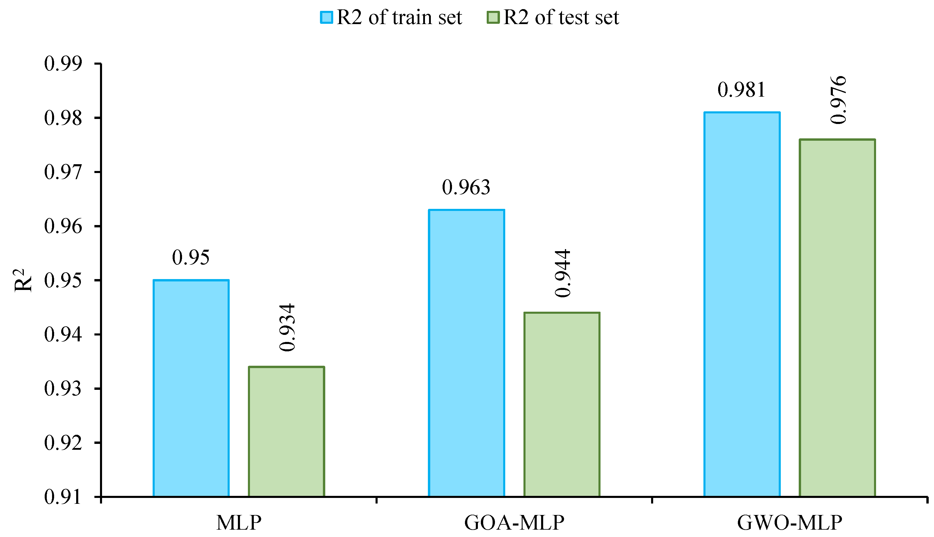
| MLP | 0.934 | 0.931 | 0.936 | 0.937 | 0.934 | 0.934 | 0.002 |
| GOA–MLP | 0.943 | 0.943 | 0.942 | 0.945 | 0.946 | 0.944 | 0.001 |
| GWO–MLP | 0.974 | 0.976 | 0.976 | 0.977 | 0.975 | 0.976 | 0.001 |
| RMSE | |||||||
| Model | Fold 1 | Fold 2 | Fold 3 | Fold 4 | Fold 5 | Mean | Std Dev |
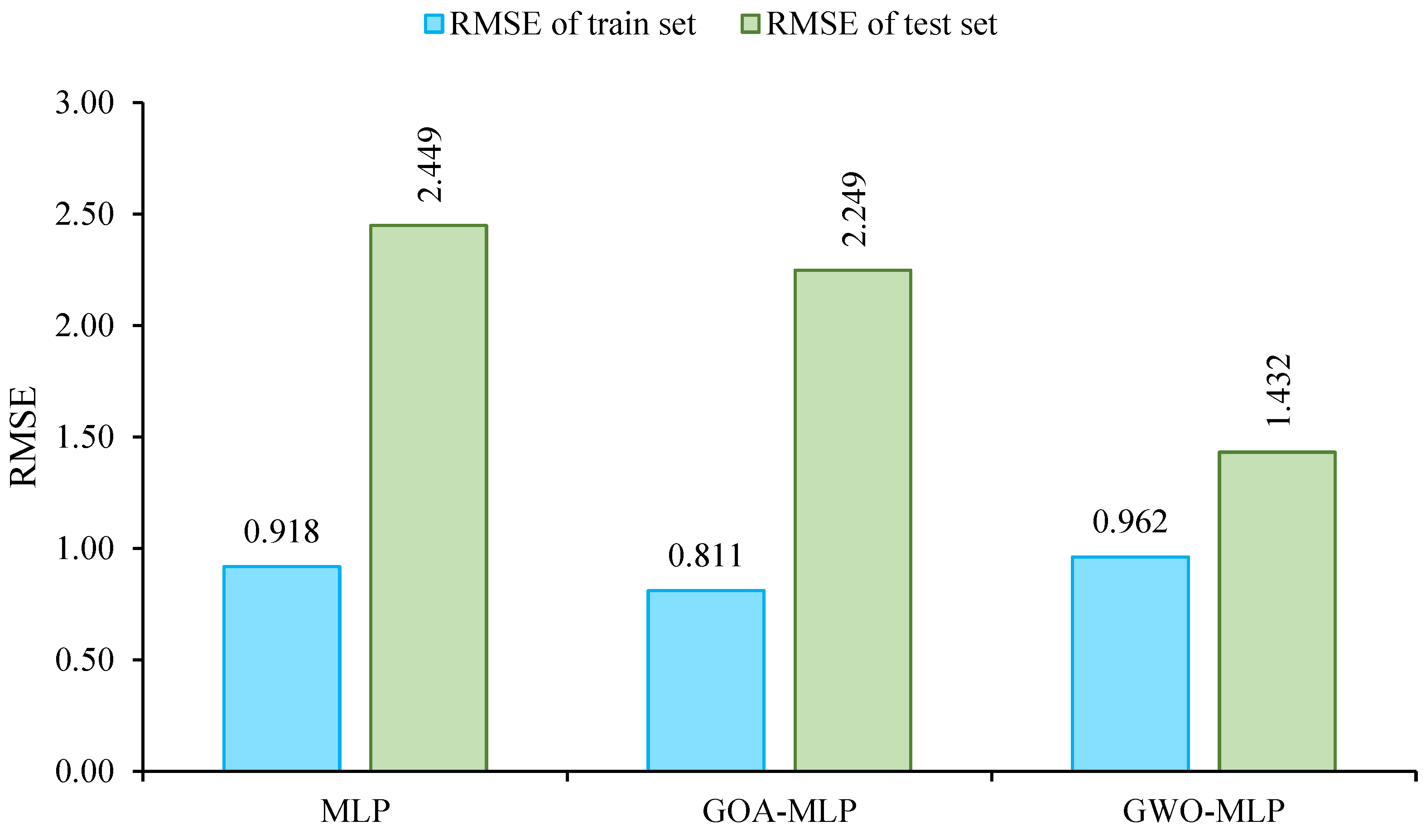
| MLP | 2.448 | 2.449 | 2.45 | 2.447 | 2.451 | 2.449 | 0.001 |
| GOA–MLP | 2.248 | 2.249 | 2.25 | 2.247 | 2.251 | 2.249 | 0.001 |
| GWO–MLP | 1.431 | 1.432 | 1.433 | 1.43 | 1.434 | 1.432 | 0.001 |
| VAF | |||||||
| Model | Fold 1 | Fold 2 | Fold 3 | Fold 4 | Fold 5 | VAF | Std Dev |
| MLP | 91.266 | 92.266 | 93.266 | 94.266 | 95.266 | 93.266 | 1.291 |
| GOA–MLP | 90.862 | 91.862 | 92.862 | 93.862 | 94.862 | 92.862 | 1.291 |
| GWO–MLP | 95.507 | 96.507 | 97.507 | 98.507 | 99.507 | 97.507 | 1.291 |
| Technique | Train Phase | Test Phase | Train Phase | Test Phase | Total Rate | Rank | ||||||||
|---|---|---|---|---|---|---|---|---|---|---|---|---|---|---|
| R2 | RMSE | VAF | R2 | RMSE | VAF | R2 | RMSE | VAF | R2 | RMSE | VAF | |||
| MLP | 0.950 | 0.918 | 94.591 | 0.934 | 2.449 | 93.266 | 1 | 2 | 1 | 1 | 2 | 2 | 9 | 3 |
| GOA–MLP | 0.963 | 0.811 | 95.781 | 0.944 | 2.249 | 92.862 | 2 | 3 | 2 | 2 | 1 | 1 | 11 | 2 |
| GWO–MLP | 0.981 | 0.962 | 97.438 | 0.976 | 1.432 | 97.507 | 3 | 1 | 3 | 3 | 3 | 3 | 16 | 1 |
| Comparison | Training Phase | Testing Phase | ||
|---|---|---|---|---|
| Statistic | p-Value | Statistic | p-Value | |
| MLP vs. GOA–MLP (Train) | 493 | 0.0388474 | 29 | 0.0069727 |
| MLP vs. GWO–MLP (Train) | 175.5 | 0.0000038 | 34 | 0.0339844 |
| GOA–MLP vs. GWO–MLP (Train) | 238 | 0.0001101 | 17 | 0.0122852 |
Disclaimer/Publisher’s Note: The statements, opinions and data contained in all publications are solely those of the individual author(s) and contributor(s) and not of MDPI and/or the editor(s). MDPI and/or the editor(s) disclaim responsibility for any injury to people or property resulting from any ideas, methods, instructions or products referred to in the content. |
© 2024 by the authors. Licensee MDPI, Basel, Switzerland. This article is an open access article distributed under the terms and conditions of the Creative Commons Attribution (CC BY) license (https://creativecommons.org/licenses/by/4.0/).
Share and Cite
Wang, X.; Zhong, Y.; Zhu, F.; Huang, J. Digital Industrial Design Method in Architectural Design by Machine Learning Optimization: Towards Sustainable Construction Practices of Geopolymer Concrete. Buildings 2024, 14, 3998. https://doi.org/10.3390/buildings14123998
Wang X, Zhong Y, Zhu F, Huang J. Digital Industrial Design Method in Architectural Design by Machine Learning Optimization: Towards Sustainable Construction Practices of Geopolymer Concrete. Buildings. 2024; 14(12):3998. https://doi.org/10.3390/buildings14123998
Chicago/Turabian StyleWang, Xiaoyan, Yantao Zhong, Fei Zhu, and Jiandong Huang. 2024. "Digital Industrial Design Method in Architectural Design by Machine Learning Optimization: Towards Sustainable Construction Practices of Geopolymer Concrete" Buildings 14, no. 12: 3998. https://doi.org/10.3390/buildings14123998
APA StyleWang, X., Zhong, Y., Zhu, F., & Huang, J. (2024). Digital Industrial Design Method in Architectural Design by Machine Learning Optimization: Towards Sustainable Construction Practices of Geopolymer Concrete. Buildings, 14(12), 3998. https://doi.org/10.3390/buildings14123998