Statistical Evaluation of Uniform Temperature and Thermal Gradients for Composite Girder of Tibet Region Using Meteorological Data

Abstract

To accurately assess the temperature action and effect of steel-concrete composite girder bridges in plateau and cold areas, this paper investigated nearly 50 years of historical meteorological data from 26 meteorological observation stations in the Tibet region of China. Based on the most unfavorable extreme meteorological data at each meteorological station, a finite element model was used to analyze the temperature field of the composite girder. The most unfavorable values of temperature were obtained. The regional differences in temperature actions at different meteorological stations were analyzed, and the isotherm maps of the extreme values of the uniform temperature and thermal gradients were further obtained based on spatial interpolation methods in the ArcGIS program. The study shows that the uniform temperature is significantly affected by the climatic environment, and the isotherm maps provide a visual representation of the geographic distribution pattern of temperature extremes. The maximum and minimum uniform temperatures in Tibet range from 18.28 °C to 42.27 °C and from −41.07 °C to 4.71 °C respectively. The maximum regional difference of positive and negative thermal gradient reaches 11.32 °C and 7.69 °C respectively. The temperature effects calculated using the most unfavorable values of the isotherm map are all more unfavorable than the specification calculations. In particular, the tensile stress of the concrete under the positive thermal gradient reaches 2.91 MPa, which exceeds the standard value of the tensile strength of concrete. This is a significant risk factor for cracking. The compressive stress of the steel girder under a negative thermal gradient reaches 19.35 MPa, which represents a 136% increase compared to the specified value. This increase elevates the risk of instability in the steel girder.

1. Introduction

Steel-concrete composite girders can fully exploit the advantages of two materials, steel and concrete. Due to the advantages of low weight, high load capacity, good dynamic performance, ease of construction and lower cost, steel-concrete composite girders have become a very competitive bridge type for small and medium-span bridges [1].

Bridge structures exposed to the environment are directly affected by solar radiation, air, temperature and wind speed. The temperature action has a significant impact on the safety and durability of bridges [1,2,3]. The composite girder consists of two types of materials with the thermal conductivity of steel being much higher than that of concrete, which makes the temperature effect more complicated than that of concrete bridges. Temperature actions in bridges can be divided into two categories, in which the uniform temperature action controls the longitudinal deformation of the main girder, which is a key factor in determining the length of the girder bridge splitting coupling as well as the selection of the bearing and expansion joints [4,5], and unreasonably uniform temperatures may result in increased manufacturing costs for bearings and expansion joints. The other category is the thermal gradient action, the thermal stress caused by the non-uniformity of the temperature distribution of the cross-section is an important cause of concrete cracking [6,7].

The temperature-action value obtained in a particular region is often difficult to apply to other regions due to significant regional differences in meteorological conditions. Therefore, it is reasonable to suggest that full consideration of the regional differences in meteorological factors for zoning values is essential. National codes have made provisions for regional differences in the uniform temperature extremes of concrete main girders. The AASHTO-LRFD specification employs two methodologies to account for the uniform temperature extremes of concrete main girders [8]. The first method delineates the United States into cold and mild regions, thereby establishing the uniform temperature extremes of concrete bridges in each region. The second method presents an isothermal map of the design temperature extremes of concrete bridges across the United States. The Eurocode [9] provides the uniform temperature extremes of concrete bridges based on the shade air temperature extremes, which are obtained through isothermal plots. The General Specifications for Design of Highway Bridges and Culverts divides China into three regions based on temperature extremes: extremely cold, cold, and warm. It stipulates the uniform temperature extremes for bridges in each region and refers to the British specification to give the formula for calculating the uniform temperature extremes based on the average daily temperature extremes of the local calendar year. National Railway Administration of the People’s Republic of China Code for design on railway bridges and culverts (TB 10002-2017) [10] establishes the uniform temperature extremes based on the style and size of the structure and the local outside air temperature, among other factors. The outside air temperature is determined based on the national average air temperature charts for January and July. A review of the aforementioned codes reveals that, with the exception of the General Specifications for Design of Highway Bridges and Culverts, the remaining codes employ the isothermal map to calculate uniform temperature extremes. In comparison to the zonal value of temperature actions, the isothermal map represents a more precise methodology for accounting for the regional differences of temperature actions in the context of value determination. It can thus be concluded that the zoning method employed in the General Specifications for Design of Highway Bridges and Culverts may result in the determination of inaccurate values for the uniform temperature extremes.

The systematic investigation of thermal gradient research also shows obvious regional variations [11], paralleling those seen in uniform temperatures. Potgieter et al. [12] employed numerical simulation based on historical meteorological data from 26 meteorological stations in the United States to investigate the role of thermal gradients for concrete box girders in different regions of the United States. Accordingly, the AASHTO code subdivides the United States into four regions for the purpose of thermal gradient consideration, based on the level of solar radiation intensity. Mirambell [13] provided isotherm maps for the temperature difference taken of concrete girders in cross-sections in different regions of the Iberian Peninsula, taking into account various meteorological parameters in the summer season. In contrast, Liu Jiang et al. [14] divided China into four regions for thermal gradient taking by establishing a correlation between the temperature action of concrete box girders and geographic and meteorological parameters in terms of cities. The General Specifications for Design of Highway Bridges and Culverts stipulates that the thermal gradient action in different regions be taken as the same value, without considering the regional differences. With the development of bridge construction to the cold region, the codal specified values of uniform temperature and thermal gradient for the design of composite girders may lead to non-conservatism in design, which brings a a great risk for the safety and durability of bridges in extreme regions. The implementation of the ‘One Belt, One Road’ initiative and the ‘Western Development Strategy’ is facilitating the gradual extension of construction activities to the cold regions of the plateau. In the construction of the Qinghai-Tibet Plateau Golmud to Lhasa section of the highway, approximately 125 km of bridge will be constructed using composite girder bridges, marking the first instance of composite girder bridges being built at such an altitude. The construction of bridges in the plateau and cold regions is subject to the dual challenges of extreme solar radiation and extreme air temperature. The temperature-related effects are more complex and pronounced, with the detrimental impact on bridge safety being particularly pronounced in these harsh environments.

It is time-consuming and laborious to measure the meteorological data and the temperature field of the main girder cross-section in different areas on site, and it is impossible to measure the temperature data at all locations of the main girder cross-section and the temperature field of the main girder cross-section under the extreme meteorological conditions due to the limited number of measuring points and the length of monitoring time [15,16,17,18]. Therefore, in the absence of on-site measured meteorological information, the use of long-term historical meteorological data from meteorological stations to simulate the temperature field of the bridge cross-section under extreme meteorological conditions has become the key to accurately predicting the value of the bridge temperature action [19,20].

In this paper, 26 meteorological observation stations in Tibet, China, were investigated for nearly 50 years of historical meteorological data. Based on the most unfavorable meteorological data at each meteorological station, a finite element model was used to analyze the temperature field of the composite girder. The most unfavorable values of uniform temperature and positive and negative vertical thermal gradients were obtained. Then, the regional differences of the temperature actions at different meteorological stations are analyzed, and the Isotherm maps of the extreme values of the uniform temperature and thermal gradient actions are further obtained by using the spatial interpolation method, which improves the accuracy of the temperature actions. Related research can provide guidance for the refined design of composite girder bridges.

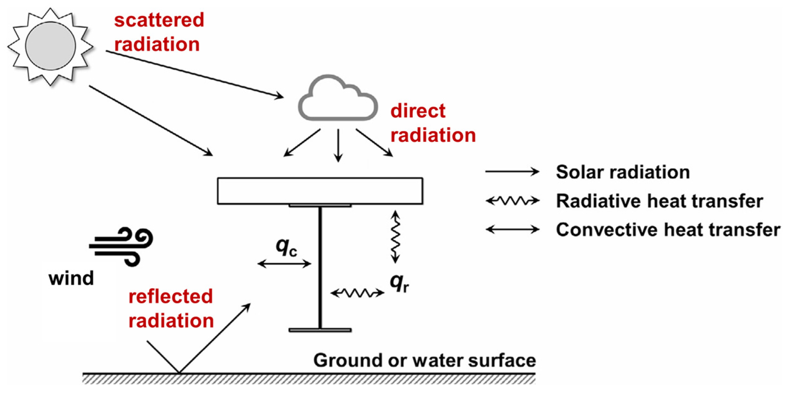
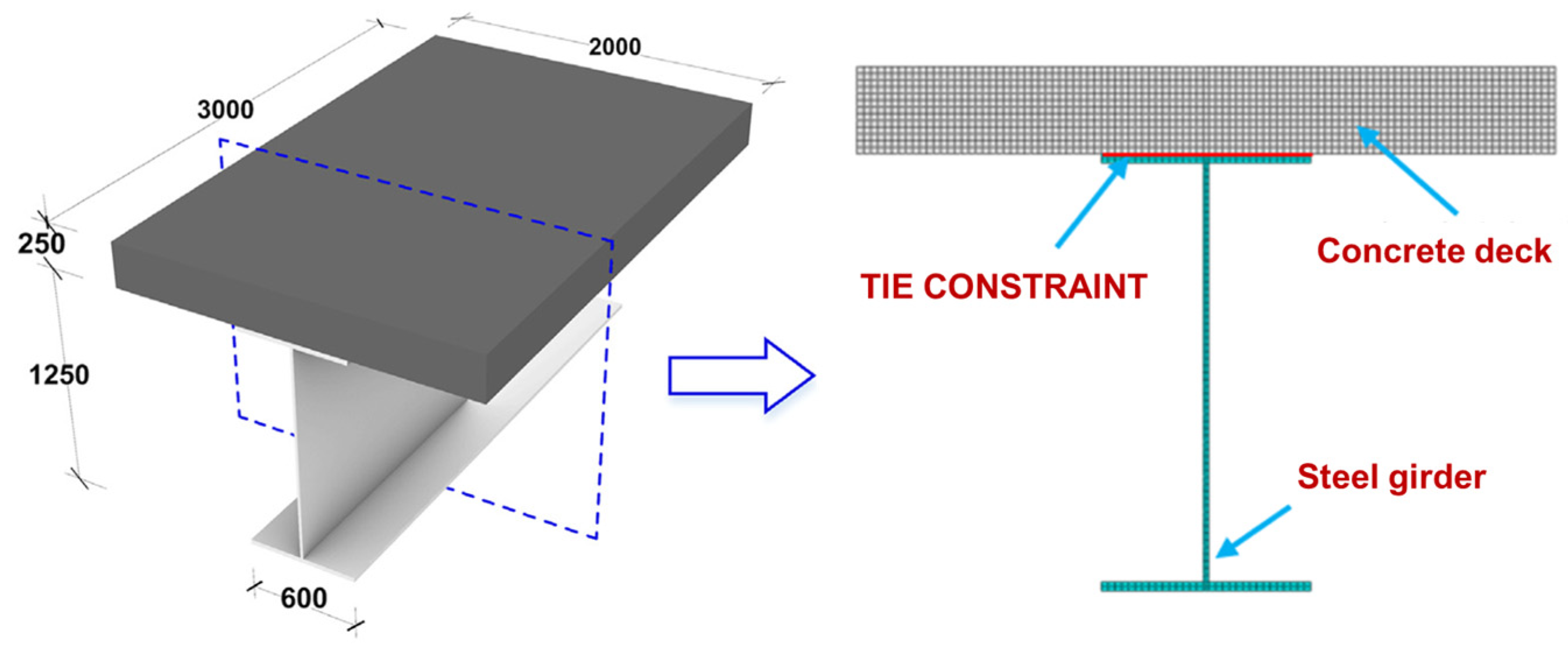
2. Numerical Simulation Method for Temperature Field

The temperature distribution of a bridge structure under insolation depends on both heat exchange with the outside world and heat conduction inside. The accuracy of numerical simulation results also depends on this [21,22].

Solving the temperature field of a bridge structure involves addressing a spatial heat conduction problem. The heat conduction within the bridge structure is governed by the partial differential equation for heat conduction proposed by Fourier (see Equation (1)).

$$\rho c{\displaystyle \frac{\partial T}{\partial t}}={\displaystyle \frac{\partial }{\partial x}}\left(k{\displaystyle \frac{\partial T}{\partial x}}\right)+{\displaystyle \frac{\partial }{\partial y}}\left(k{\displaystyle \frac{\partial T}{\partial y}}\right)+{\displaystyle \frac{\partial }{\partial z}}\left(k{\displaystyle \frac{\partial T}{\partial z}}\right)+Q$$

(1)

where: t, x, y, z are the time and space coordinates; T is the temperature of the bridge; ρ, is the density, c, is specific heat capacity, k is thermal conductivity; Q is the heat generated by the structure per unit of volume of itself.

The transfer of heat between the bridge structure and the external environment under the influence of solar radiation is primarily attributable to three mechanisms: solar radiation, convection heat transfer, and radiation heat transfer. This phenomenon represents the boundary condition for the solution of the aforementioned partial differential equation of heat transfer. For further clarification, please refer to Figure 1. See Appendix A for detailed calculations.

3. Temperature Actions on Composite Girder Bridges

3.1. Uniform Temperature

The temperature of a composite girder section can be categorized into four parts: uniform temperature, transverse linear temperature difference, vertical linear temperature difference, and residual temperature difference [15], where the uniform temperature causes longitudinal elongation and shortening of the bridge. Composite girder consists of two materials with very different thermophysical properties, steel and concrete, the temperature-induced longitudinal deformation of the steel girder and concrete deck slab must be coordinated, and its uniform temperature can be calculated by the following equation [15].

$$T_{\mathrm{e}}={\displaystyle \frac{{\displaystyle \sum E_{\mathrm{s}}{A}_{\mathrm{s}\mathrm{i}}}{T}_{\mathrm{s}\mathrm{i}}+{\displaystyle \sum E_{\mathrm{c}}{A}_{\mathrm{c}\mathrm{i}}{T}_{\mathrm{c}\mathrm{i}}}}{{\displaystyle \sum E_{\mathrm{s}}{A}_{\mathrm{s}\mathrm{i}}}+{\displaystyle \sum E_{\mathrm{c}}{A}_{\mathrm{c}\mathrm{i}}}}}$$

(2)

where T_e is the uniform temperature of the composite girder section, E_s and E_c are the modulus of elasticity, and T_si, T_ci, A_si, and A_ci are the temperature value and cross-sectional area, respectively.

3.2. Thermal Gradient

The nonlinear temperature difference in the bridge cross-section due to daytime warming and nighttime cooling is usually defined as positive and negative thermal gradients, respectively.

The thermal gradient curves of bridges can generally be expressed in the form of multiple parabolas, exponential curves and multifolds, which can better reflect the effect of insolation on the warming of the top of bridges, in which the Chinese JTG D60-2015 [23], AASHTO and Eurocode-1 general model adopt the form of bifold line.

For the negative thermal gradient mode, China JTG D60-2015 and AASHTO take −0.5 and −0.3 of the respective positive thermal gradient, respectively. Only the general mode of Eurocode-1 considers that there exists an obvious nonlinear distribution of temperature on the steel girder. The measured and calculated studies have shown that the negative thermal gradient model of Eurocode-1 is more in line with the form of temperature distribution of the composite girder at night or cold wave cooling, in the daytime sunshine the concrete temperature is higher than that of the steel girder, at night or cold wave cooling, the top of the concrete deck plate cools down quickly while the interior cools down slowly, forming a negative temperature difference in the bridge deck plate, while the heat conductivity of the steel girder is about 50 times of that of the concrete deck plate. The temperature drops rapidly, but not as rapidly at the top where it is connected to the concrete; so a significant negative temperature difference is formed at the top of the steel girder.

For comprehensive consideration, the positive thermal gradient model in China JTG D60-2015 is selected for the subsequent analysis, which is more in line with the characteristics of China’s climate environment. Eurocode-1 negative thermal gradient model is selected for negative thermal gradient analysis, which better reflects the temperature distribution characteristics of composite girders under cooling conditions (see Figure 2).

4. Temperature Action Extremes Based on Meteorological Data

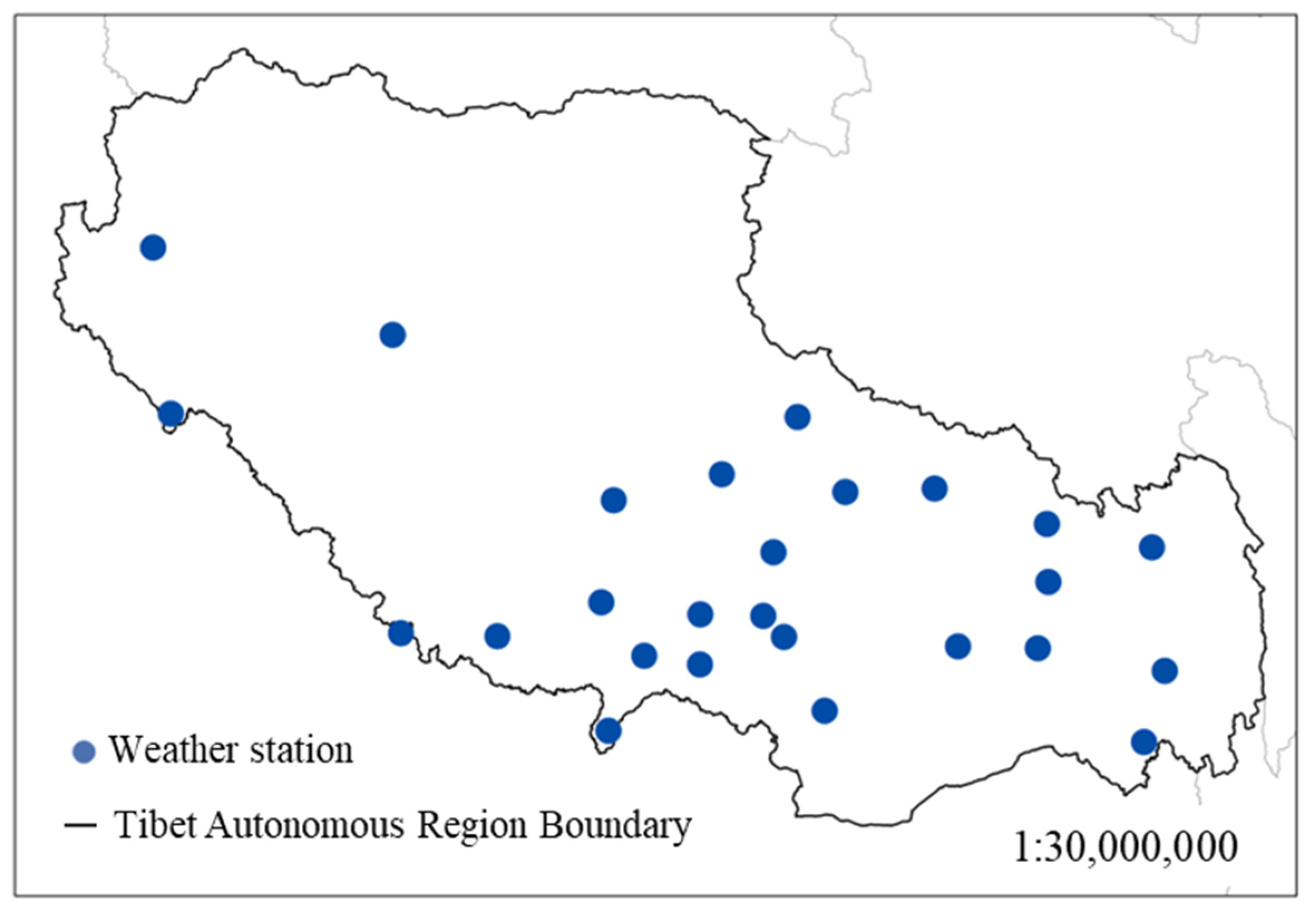
4.1. Historical Meteorological Data Research

The temperature of the bridge structure is significantly affected by environmental factors; in order to investigate the differences in temperature actions in different regions, 26 meteorological stations were collected, and the distribution of those is shown in Figure 3. The meteorological data collected include daily maximum and minimum temperatures, daily average wind speed and total solar radiation. The meteorological data cover the period from 1 January 1953 to 31 December 2015. Meteorological data have been processed for outliers using the Hampel filter method [24].

4.2. Extreme Meteorological Conditions

It is essential to ascertain the impact of extreme temperature on the bridge by analysing meteorological data representing extreme conditions. Consequently, an extreme value analysis was conducted using long-term data on air temperature, solar radiation, and wind speed, resulting in the identification of extreme meteorological values for each meteorological station over a 100-year period. These values exhibited a normal distribution with a 95% confidence level. The daily value data were decomposed into hourly segments using the methodology in the literature [25,26].

A sinusoidal function is used to simulate the daily ambient temperature profile. When the daily maximum temperature T_max and daily minimum temperature T_min are known, the temperature at any moment of the day can be obtained by the following formula [27,28].

$$T\left(t\right)={\displaystyle \frac{T_{\max }+T_{\min }}{2}}+{\displaystyle \frac{T_{\max }-T_{\min }}{2}}\sin \left[\left(t-t_0\right){\displaystyle \frac{\pi }{12}}\right]$$

(3)

where, T(t) is the daily change of air temperature; T_max and T_min are the Maximum and minimum air temperature; t₀ indicates the time of occurrence of the maximum and minimum temperatures.

4.3. Extreme Value Calculation of Temperature Action

4.3.1. Computational Models

The quadrilateral heat-transfer element DC2D4 with 4-node was employed for the modelling of the cross-section. The dimensions of the element were selected to be approximately 3.0 × 2.5 cm and 3.0 × 1.0 cm for the concrete deck and steel beam, respectively, with a total of 848 elements and 1014 nodes over the cross-section. The interface between the concrete deck and the steel girder in the model was defined as a bond constraint, ensuring the continuity of temperature and heat flux at the interface, which is a reasonable approximation [29]. The finite element model is illustrated in Figure 4 and the thermal parameters of steel, concrete and asphalt in the model are shown in

Table 1. Material properties used in FE analysis.

Characteristics	Steel	Concrete
Density $\rho /(\mathrm{k}g\cdot {\mathrm{m}}^{-3})$	7840	2150
Specific heat capacity $c/[\mathrm{J}/\left(\mathrm{kg}\cdot °\mathrm{C}\right)]$	465	910
Thermal conductivity $\lambda /[W/\left(\mathrm{m}\cdot °\mathrm{C}\right)]$	55	2.8
Absorptivity $\xi$	0.5	0.45
Emittivity $\epsilon$	0.8	0.85

.

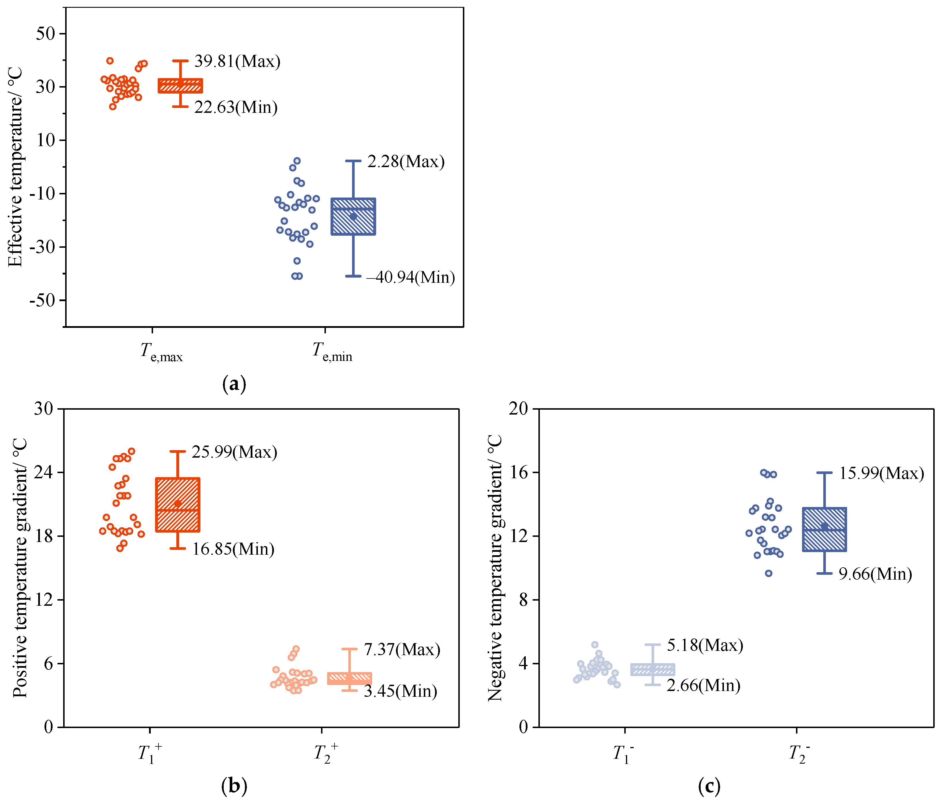
4.3.2. Calculation Results

Based on the aforementioned extreme meteorological conditions setting method, the most unfavorable meteorological boundary conditions of 26 meteorological stations in Tibet were obtained. ABAQUS 6.14 software is used to establish the temperature field calculation model of the composite girder. Finally, each meteorological station has uniform temperature and thermal gradient extremes, see

Table 2. Extreme value of temperature actions in Tibet.

Meteorological Station Information			Geographic Information			Uniform Temperature/°C		Positive Gradient/°C		Negative Gradient/°C
Serial	Station Number	Name of Meteorological Station	Latitude	Longitude	Altitude/m	Te,max	Te,min	T1+	T2+	T1−	T2−
1	55228	Shiquan River	32.3	80.05	4278.6	33.00	−35.25	25.50	6.91	4.22	14.19
2	55248	Gerze	32.09	84.25	4414.9	32.69	−40.94	25.30	6.56	5.18	13.90
3	55279	Bangor	31.23	90.01	4700	29.53	−40.94	25.30	3.45	3.60	15.87
4	55294	Amdo	32.21	91.06	4800	26.51	−25.24	25.30	4.34	3.47	15.87
5	55299	Nagchu	31.29	92.04	4507	27.22	−26.66	25.99	5.18	4.63	13.19
6	55437	Burang	30.17	81.15	3900	28.26	−27.07	21.80	3.90	3.76	11.03
7	55472	Shenzha	30.57	88.38	4672	30.84	−24.39	21.80	7.37	3.35	11.03
8	55493	Dangxiong	30.29	91.06	4200	27.42	−24.51	22.85	5.09	3.90	13.16
9	55578	Shigatse	29.15	88.53	3836	31.27	−13.33	18.50	4.21	3.81	12.43
10	55585	Nimu	29.26	90.1	3809.4	31.45	−15.15	18.24	4.14	3.76	12.42
11	55591	Lhasa	29.4	91.08	3648.9	32.02	−14.03	18.38	4.09	3.36	11.08
12	55598	Tsedang	29.16	91.46	3560	32.52	−10.42	18.47	4.24	3.45	11.53
13	55655	Nyalam	28.11	85.58	3810	33.45	−11.74	18.47	4.42	3.16	9.66
14	55664	Tingri	28.38	87.05	4300	25.21	−15.35	21.80	5.02	4.03	15.99
15	55680	Gyangzê	28.55	89.36	4040	28.07	−20.30	21.10	4.82	3.94	12.33
16	55681	Nankazi	28.58	90.24	4431.7	30.59	−16.17	18.89	4.19	3.30	11.03
17	55696	Lhunzi	28.25	92.28	3860	22.63	−28.96	19.76	4.46	4.23	13.76
18	55773	Pari	27.44	89.05	4300	29.28	−14.42	19.76	5.07	3.82	13.76
19	56106	Suo County	31.53	93.47	4022.8	39.81	−5.20	19.09	4.19	3.65	11.74
20	56116	Tingqing	31.25	95.36	3873.1	29.49	−23.70	22.73	4.36	2.87	12.04
21	56137	Chamdo	31.09	97.1	3315	36.90	−11.92	24.50	5.42	3.98	13.57
22	56223	Lhokhorn	30.45	95.5	3640	26.08	−22.24	23.43	4.45	2.98	12.17
23	56227	Bomi	29.52	95.46	2736	32.34	−12.31	18.47	3.95	3.09	12.18
24	56312	Linzhi	29.4	94.2	2991.8	38.52	−0.35	17.33	4.01	3.40	10.86
25	56331	Zuogang	29.4	97.5	3780	32.87	−6.13	18.18	3.73	2.97	12.42
26	56434	Qasumi	28.39	97.28	2327.6	38.79	2.28	16.85	3.46	2.66	10.80

. To illustrate, the change pattern of the maximum and minimum uniform temperatures within a day at the Linzhi station is presented in Figure 5.

5. Temperature Actions Extremes Based on Geographic Variation

5.1. Regional Differences in Temperature Actions

The box plots of the results of uniform temperature and thermal gradient calculations for the composite girders are given in Figure 6, and the maximum and minimum values of each temperature action in the 26 meteorological stations are indicated. It can be clearly seen that the representative values of each temperature action have significant variability in each station. Among them, the values of T_e,max and T_e,min in the 26 stations range from 22.63 to 39.81 °C and −40.94 to −2.28 °C, respectively, and the maximum difference between stations reaches 17.18 °C and 43.22 °C, respectively; the values of T₁⁺ and T₂⁺ in the positive thermal gradient range from 16.85 to 25.99 °C and 3.45 to 7.37 °C, respectively, with the maximum difference reaching 9.14 °C. The values of T₁⁺ and T₂⁺ in the positive thermal gradient ranged from 16.85 to 25.99 °C and 3.45 to 7.37 °C, with the maximum difference of 9.14 °C and 3.92 °C, respectively; the values of T₁⁻ and T₂⁻ in the negative thermal gradient ranged from 2.66 to 5.18 °C and 9.66 to 15.99 °C, with the maximum difference of 2.52 °C and 6.33 °C, respectively; and the regional differences of T_e,min was the most significant.

5.2. Isotherm Maps of Extreme Temperatures Actions

On the basis of the long-term calculation of the temperature-action representative values of the 26 stations using finite elements, the spatial interpolation calculation is carried out by using ArcGIS 10.7 software, and the temperature action Isotherm maps are further drawn. To ensure that the data of the sample points remain unchanged after spatial interpolation and that the interpolation curve is smooth, spatial interpolation calculation using the spline function method averaging is performed.

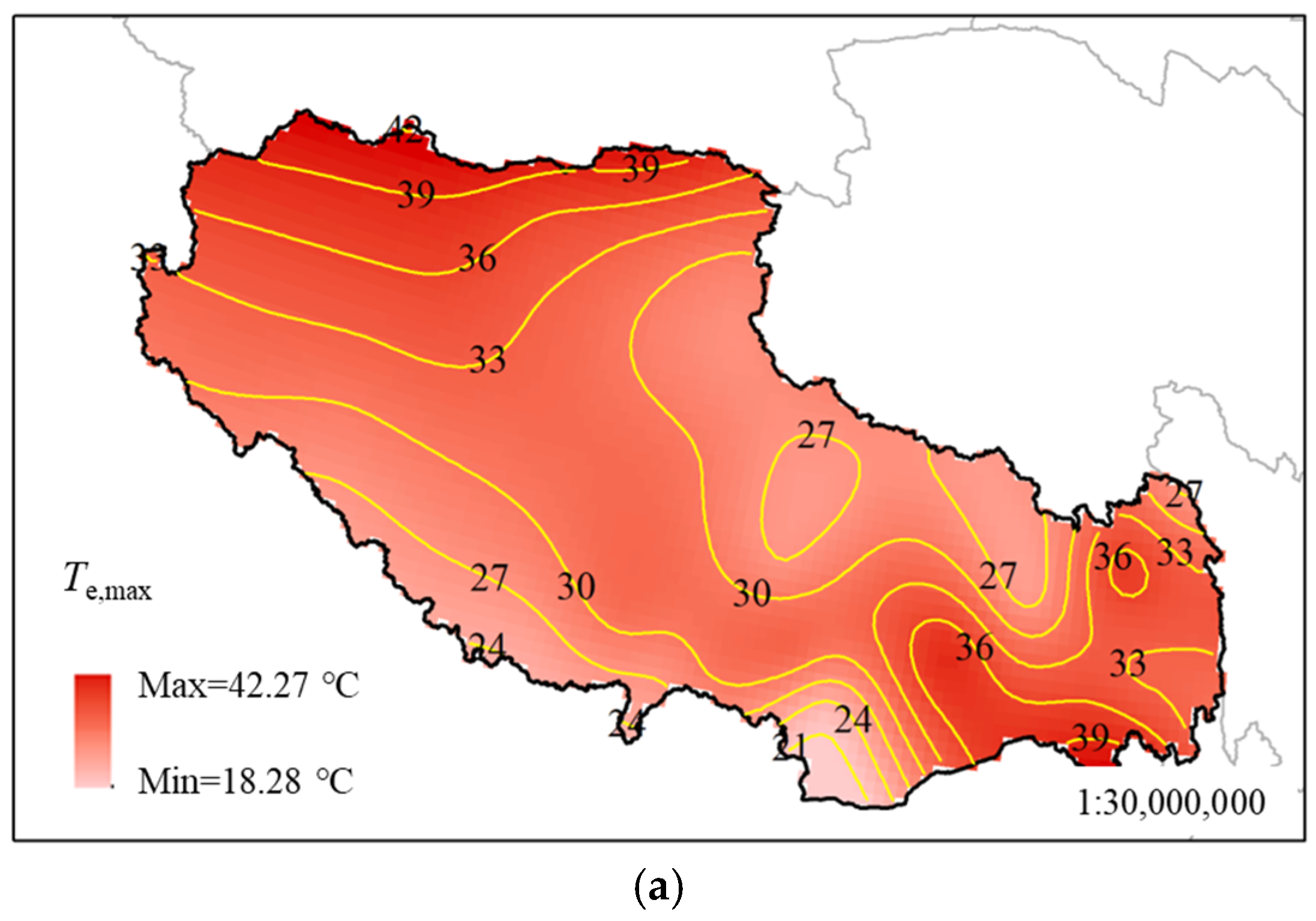
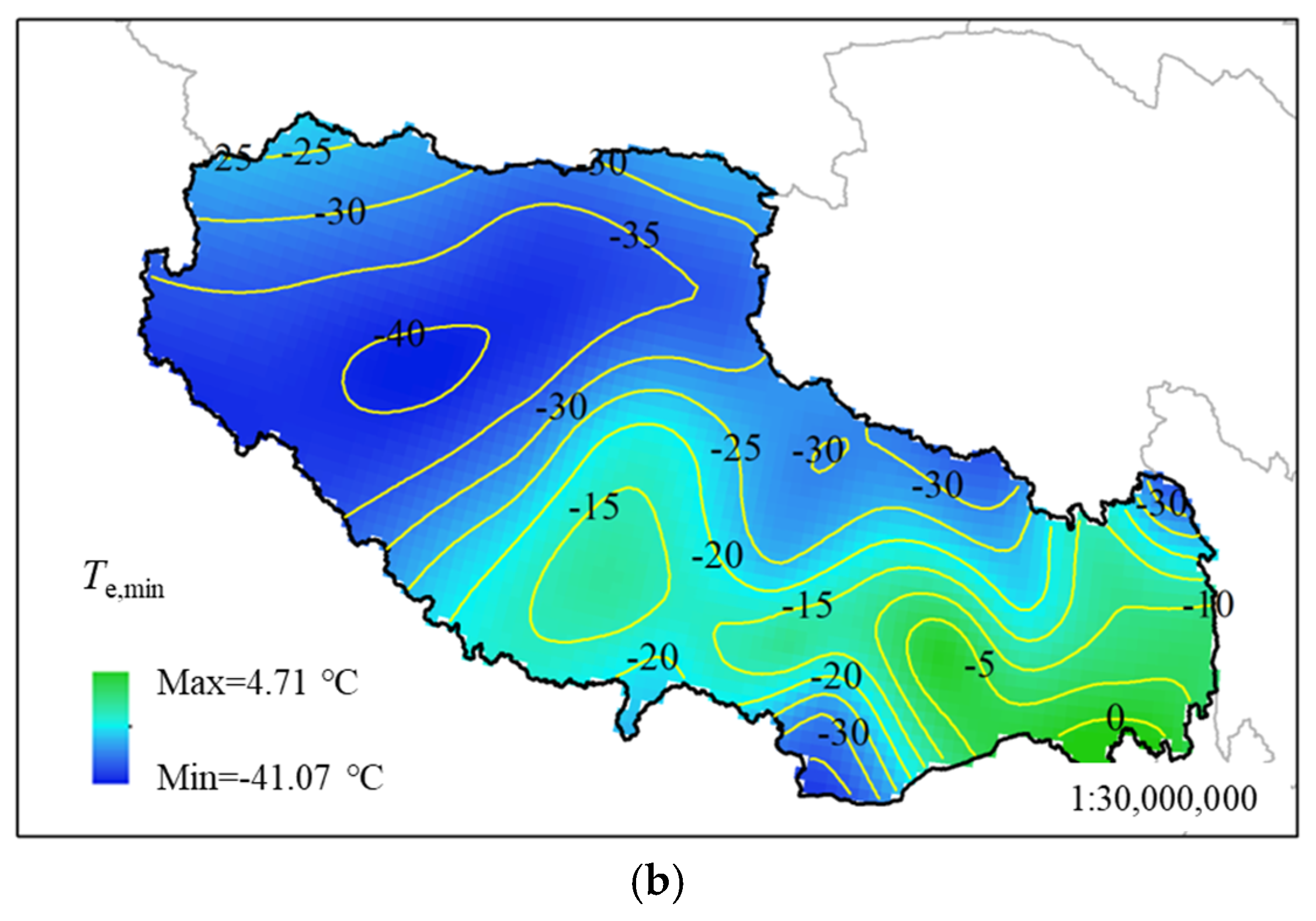
5.2.1. Uniform Temperature

The Isotherm map of the maximum uniform temperature in Tibet is plotted in Figure 7a. For the uniform temperature T_e, the interpolated maximum uniform temperature T_e,max takes values ranging from 18.28 °C to 42.27 °C, and the range of variation is slightly larger than that of the finite element calculation results, which also explains the reasonableness of the spatial interpolation method to some extent. Among them, the highest T_e,max occurs at the junction of northern Tibet and Xinjiang Tarim Basin, and the T_e,max is also larger at the junction of eastern Tibet and Sichuan and Yunnan. This is due to the fact that the uniform temperature is mainly affected by the annual average temperature, and these areas have lower altitudes and higher temperatures. The lowest T_e,max occurs at the border of southwest Xinjiang and India, which is located on the Tibetan Plateau and has lower annual temperatures. Figure 7b shows the Isotherm map of the minimum uniform temperature, and it can be seen that the value of the minimum uniform temperature, T_e,min, ranges from −41.07 °C to 4.71 °C. The variation range of T_e,min reaches 45.47 °C, which is significantly higher than that of the maximum uniform temperature, T_e,min is also significantly affected by the air temperature, and the minimum value mainly occurs in the Tibetan Plateau region of northwestern Tibet, mainly due to the sharp decrease of the minimum temperature with the increase in altitude. This is mainly due to the sharp decrease in the minimum temperature with the increase in altitude.

Figure 8 shows the zoning map of the uniform temperature in the General Specifications for Design of Highway Bridges and Culverts, and the comparison with the General Specifications for Design of Highway Bridges and Culverts, it can be seen that in the General Specifications for Design of Highway Bridges and Culverts, the northern part of Tibet is in the cold region, the southern part is in the cold region, and the maximum uniform temperature code suggests that the values are all 39 °C, and comparing with the results of this paper, except for a few areas in the northern part of Tibet, the other areas are all less than the code suggests the value. This shows that the Chinese code for the maximum uniform temperature is safe enough, but the economy may be insufficient. The normative recommended values for the minimum uniform temperature in severe cold regions and cold regions are −32 °C and −15 °C, respectively, and the range of variation is much smaller than the calculated results of this paper, which are −41.07 °C to 4.71 °C. The minimum uniform temperature in cold regions is −41.07 °C to −4.71 °C. If the value is taken according to the specification, it is obviously too rough, and the minimum uniform temperature of the composite girder in most areas of the plateau region in northern Tibet is seriously underestimated, while the design of the composite girder bridge in the southern region of Tibet may be too conservative.

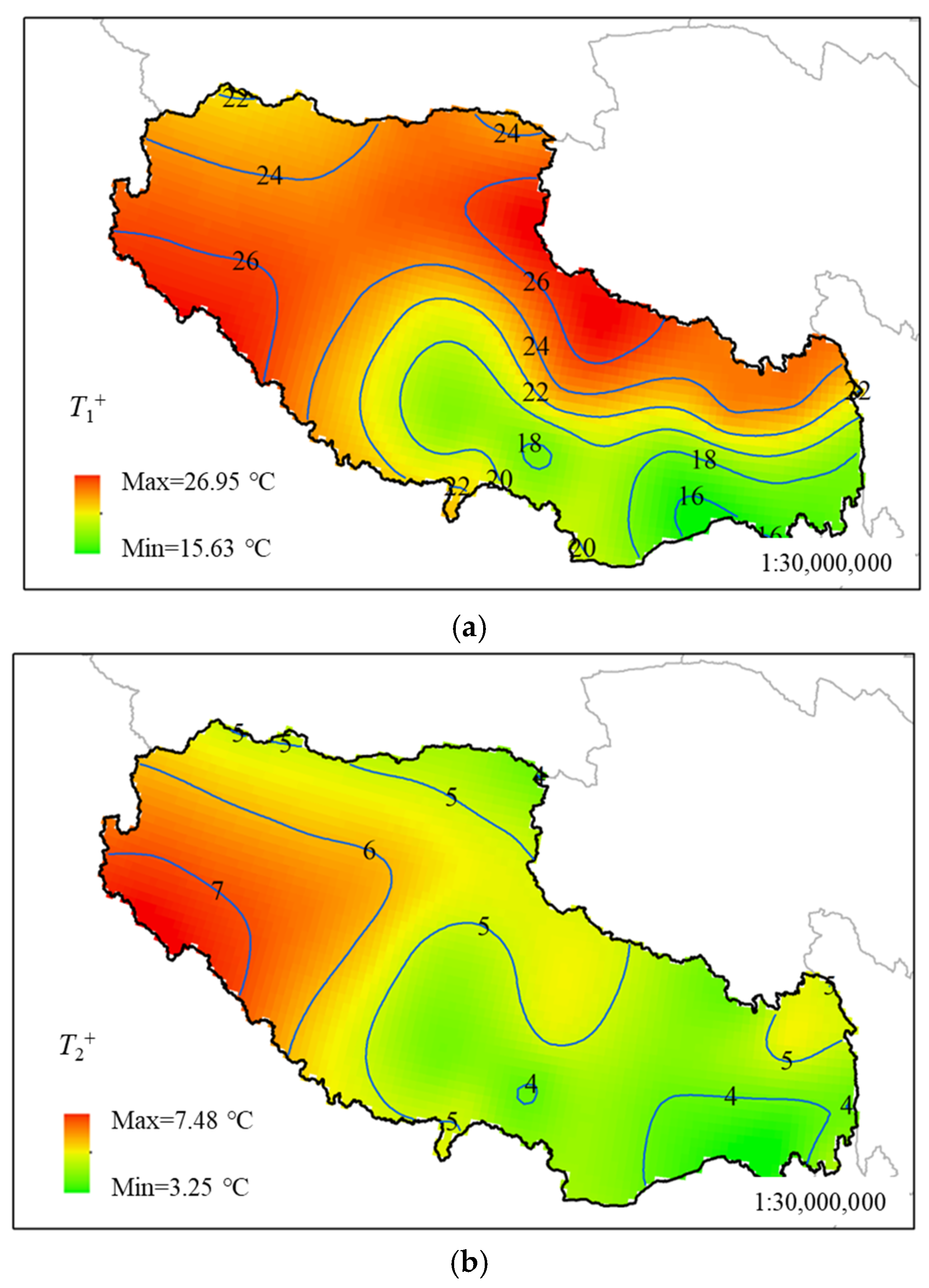
5.2.2. Positive Thermal Gradient

The national Isotherm maps of T₁⁺ and T₂⁺ in the positive thermal gradient of the composite girder bridge are plotted in Figure 9, in which the values of T₁⁺ range from 15.63 °C to 26.95 °C, with a geographic variation of 11.32 °C. The T₁⁺ is mainly caused by the solar radiation at the top of the deck slabs, which is stronger at higher elevations. Therefore, the maximum value occurs at the highest elevation in the southwestern and northeastern parts of the Tibetan Plateau. The temperature difference T₂⁺ is accompanied by T₁⁺, so the distribution pattern is similar to that of T₁⁺. However, after the heat transfer process of the concrete of the bridge deck slab, the value decreases significantly; the value of T₂⁺ ranges from 3.25 °C to 7.48 °C. The temperature difference T₂⁺ is the same as that of T₁⁺.

For the deck slab thickness of not more than 0.4 m of the composite girders, the Chinese highway specification of the top temperature difference T₁⁺ takes the value of 25 °C, which basically can cover the unfavorable value in the calculation results of this paper. However, for most areas in Tibet, the specification is still conservative, and the value of T₂⁺ is 6.7 °C, which is not more than 1 °C different from the average value of T₂⁺ calculated in this paper.

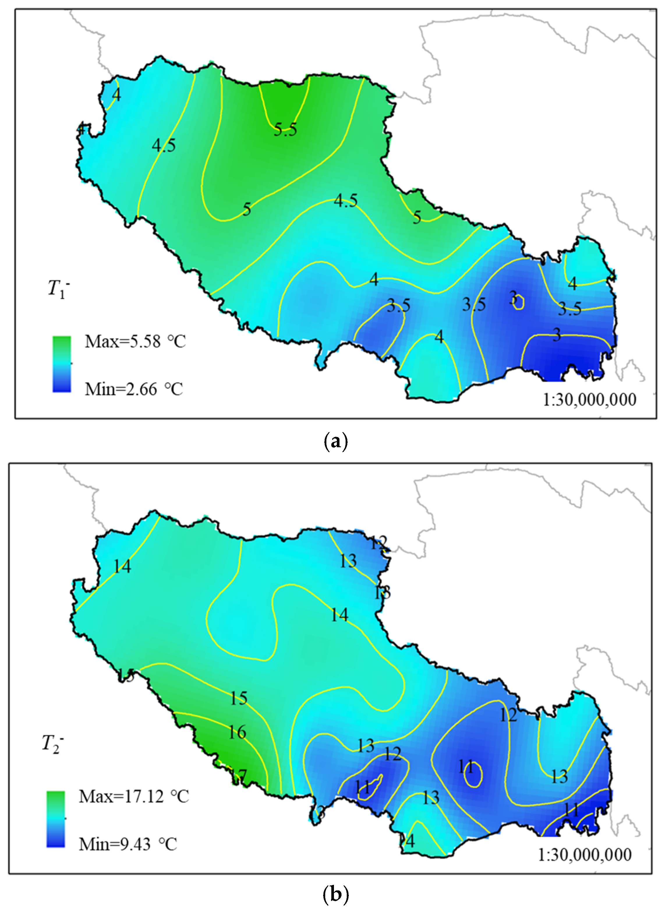
5.2.3. Negative Thermal Gradient

The national Isotherm maps of T₁⁻ and T₂⁻ in the negative thermal gradient of the composite girder bridge are plotted in Figure 10, where the values of T₁⁻ are taken in the range of 2.66 °C to 5.58 °C, and the regional differences are not significant. This phenomenon can be attributed to the inadequate thermal conductivity of concrete, which results in a negligible temperature differential within the concrete deck slab during the cooling phase. While steel girders have good thermal conductivity, steel girders cool down quickly when the temperature drops. The range of T₂⁻ values reaches 9.43~17.12 °C, and the distribution characteristics are basically the same as that of T₁⁻ values. The negative thermal gradient is mainly affected by the daily temperature difference, with larger values in the western Tibetan Plateau region and smaller values in the eastern region.

The temperature difference at the top and bottom of the composite girder in Eurocode-1 is taken as −5 °C and −8 °C, respectively, the top temperature difference with the calculation of this paper basically coincides with the results, but this paper calculates the T₂⁻ much larger than the European norms, which may be caused by the more severe climatic environment of the Tibetan Plateau region.

5.3. Comparison of Temperature Effects

In order to further illustrate the differences in structural effects caused by the differences in temperature values in different regions. Taking 3 × 30 m span steel-mixed composite girder as a case study, the maximum stresses of concrete deck slabs and steel girders are extracted by calculating the temperature effects using the maximum and minimum values in the temperature maps proposed in this paper, respectively. The results are also compared with the stress calculations using the specification temperature values. The modulus of elasticity of concrete is taken as 3.55 × 10⁴ MPa and the coefficient of linear expansion is taken as 1 × 10⁻⁵/°C, while the modulus of elasticity of steel is taken as 2.06 × 10⁵ MPa and the coefficient of linear expansion is taken as 1.2 × 10⁻⁵/°C. The values of temperature actions are shown in

Table 3. Comparison of temperature values.

Temperature Action (°C)	Uniform Temperature		Positive Thermal Gradient		Negative Thermal Gradient
	Te,max	Te,min	T1+	T2+	T1−	T2−
Specification recommended value	39	−32	25	6.7	5	8
Maximum in Isotherm map	42.27	4.71	26.95	7.48	5.58	17.12
Minimum in Isotherm map	18.29	−41.07	15.63	3.25	2.66	9.43

.

The comparative results of concrete stresses are shown in

Table 4. Comparison of concrete stresses.

Stress (MPa)	Maximum Uniform Temperature	Minimum Uniform Temperature	Positive Thermal Gradient	Negative Thermal Gradient
Specification recommended value	0.75	−1.47	2.65	1.47
Maximum in Isotherm map	0.84	−0.13	2.91	1.55
Minimum in Isotherm map	0.39	−2.01	1.77	1.13

. For static structures, the effects of uniform temperature are usually released through deformation and no thermal stresses are generated. For super-static structures, both axial expansion and temperature secondary stresses are generated. For the composite girder in this example, the maximum and minimum uniform temperatures generate tensile and compressive stresses in the deck slab, respectively. The maximum tensile stress in the concrete occurs at the upper edge of the deck slab at the pivot point. The maximum value calculated using the Isotherm map reaches 0.84 MPa, which is 12% larger compared to the calculated result of 0.75 MPa for the recommended value of the specification.

A positive thermal gradient generated a large tensile stress at the lower edge of the bridge deck slab. The calculated result using the suggested value of specification is 2.65 MPa, which is slightly smaller than the standard value of tensile strength of C50 concrete 2.74 MPa, while the calculated result using the maximum value of Isotherm map reaches 2.91 MPa, which has exceeded the standard value of tensile strength of concrete, and there is a significant risk of cracking. A negative thermal gradient in the fixed support at the upper edge of the bridge deck plate produces a smaller tensile stress, and the calculation results of this paper are closer to the specification.

The calculated results of the steel girder stresses are shown in

Table 5. Comparison of steel girder stresses.

Stress (MPa)	Maximum Uniform Temperature	Minimum Uniform Temperature	Positive Thermal Gradient	Negative Thermal Gradient
Specification recommended value	0.81	−1.13	11.41	−8.20
Maximum in Isotherm map	0.88	−0.08	12.95	−19.35
Minimum in Isotherm map	0.43	−1.47	8.03	−9.89

. The uniform temperature change did not produce significant stresses in the steel girders, and neither tensile nor compressive stresses exceeded 2 MPa. Positive and negative thermal gradients produced tensile and compressive stresses in the steel girders, respectively. The compressive stresses in the steel girders calculated using the maximum value of the Isotherm map reached 19.35 MPa, which is an increase of 136% compared to the result of 8.20 MPa calculated from the recommended value of the specification. Although the temperature-generated stresses in the steel girders are not significant, they may still increase the risk of instability of the steel girders when superimposed with vehicle loads and other environmental loads.

6. Conclusions

Isotherm maps of uniform temperature and thermal gradient action extremes have been obtained based on the most unfavorable extreme meteorological conditions by investigating nearly 50 years of historical meteorological data from 26 meteorological observation stations in Tibet of China. Results show that:

(1)

The temperature action of composite girder bridges in the cold region of the plateau is more unfavorable, and the suggested values in the specification are not safe enough for the design of composite girder bridges in the Tibetan region. The isotherm maps are more detailed and reasonable designs for composite girder bridges in Tibet.

(2)

The uniform temperature of the composite girder is significantly affected by the climatic environment. The maximum and minimum uniform temperatures in Tibet are 18.28~42.27 °C and −41.07~4.71 °C, respectively.

(3)

The positive thermal gradient in the Chinese code and the negative thermal gradient in the European code are used to describe the temperature difference characteristics of the composite girders. The values of T₁⁺ and T₂⁺ range from 15.63 °C to 26.95 °C and 3.25 °C to 7.48 °C, respectively. The temperature difference at the top is more significant.

(4)

The temperature effects calculated using the most unfavorable values of isotherm maps are more unfavorable than the specification calculations, in which the tensile stress of the concrete reaches 2.91 MPa, with a significant risk of cracking.

(5)

The isotherm maps of the temperature action of composite girder bridges in Tibet were obtained from meteorological data and the accuracy of isotherm maps should be verified and improved by placing sensors for long-term structural temperature monitoring.

References

1. Liu, J.; Liu, Y.J.; Zhang, C.Y.; Zhao, Q.H.; Lyu, Y. Temperature Action and Effect of Concrete-filled Steel Tubular Bridges: A Review. J. Traffic Transp. Eng. (Engl. Ed.) 2020, 7, 174–191. [Google Scholar] [CrossRef]
2. Liu, J.; Liu, Y.J.; Jiang, L.; Zhang, N. Long-term Field Test of Thermal gradients on the Composite Girder of a Long-span Cable-stayed Bridge. Adv. Struct. Eng. 2019, 22, 2785–2798. [Google Scholar] [CrossRef]
3. Kim, S.H.; Park, S.J.; Wu, J.; Won, J.H. Temperature variation in steel box girders of cable-stayed bridges during construction. J. Constr. Steel. Res. 2015, 112, 80–92. [Google Scholar] [CrossRef]
4. Elbadry, M.M.; Ghali, A. Temperature Variations in Concrete Bridges. J. Struct. Eng. 1983, 109, 2355–2374. [Google Scholar] [CrossRef]
5. Ding, Y.; Zhou, G.; Li, A.; Wang, G. Thermal Field Characteristic Analysis of Steel Box Girder Based on Long-term Measurement Data. Int. J. Steel Struct. 2012, 12, 219–232. [Google Scholar] [CrossRef]
6. Zhang, N.; Liu, Y.J.; Liu, J. Temperature Effects of H-shaped Concrete Pylon in Arctic-alpine Plateau Region. J. Traffic Transp. Eng. 2017, 17, 66–77. [Google Scholar]
7. Badar, J.; Umar, T.; Akbar, M.; Abbas, N.; Shahzad, Q.; Chen, W.; Arshid, M.U. Innovative Methods to Improve the Seismic Performance of Precast Segmental and Hybrid Bridge Columns under Cyclic Loading. Buildings 2024, 14, 1594. [Google Scholar] [CrossRef]
8. The American Association of State Highway and Transportation Officials (AASHTO). AASHTO LRFD Bridge Design Specification; American Association of State Highway and Transportation Officials: Washington, WA, USA, 2012. [Google Scholar]
9. EN 1991-1-5; Eurocode 1: Actions on structures-Part 1-5: General Actions-Thermal Actions. European Committee for Standardization (CEN): Brussels, Belgium, 2003.
10. TB 10002-2017; National Railway Administration of the People’s Republic of China. Code for Design on Railway Bridge and Culvert. China Railway Publishing House: Beijing, China, 2017.
11. Umar, T. Making future floating cities sustainable: A way forward. Proc. Inst. Civ. Eng.-Urban Des. Plan. 2020, 173, 214–237. [Google Scholar] [CrossRef]
12. Potgieter, I.C.; Gamble, W.L. Nonlinear Temperature Distributions in Bridges at Different Locations in the United States. PCI J. 1989, 34, 80–103. [Google Scholar] [CrossRef]
13. Mirambell, E.; Aguado, A. Temperature and stress distributions in concrete box girder bridges. J. Struct. Eng. 1990, 116, 2388–2409. [Google Scholar] [CrossRef]
14. Liu, J.; Liu, Y.J.; Bai, Y.X. Study on Regional Difference and Zoning of the Thermal gradient Pattern of Concrete Box Girder. China J. Highw. Transp. 2020, 33, 73–84. [Google Scholar]
15. Quan, C. Effects of Thermal Loads on Texas Steel Bridges; University of Texas Library: Austin, TX, USA, 2008; Available online: https://www.proquest.com/openview/591e28df629caca6ddb99e845e1a143c/1?pqorigsite=gscholar&cbl=18750 (accessed on 25 November 2024).
16. Liu, J.; Liu, Y.; Ma, Z.; Zhang, G.; Lyu, Y. Thermal gradient Action of Steel-concrete Composite Girder Bridge: Action Pattern and Extreme Value Analysis. China J. Highw. Transp. 2022, 35, 269–286. [Google Scholar] [CrossRef]
17. Liu, Y.; Liu, J. Review on temperature action and effect of steel-concrete composite girder bridge. J. Traffic Transp. Eng. 2020, 20, 42–59. [Google Scholar] [CrossRef]
18. Zhang, C.; Liu, Y.; Liu, J.; Yuan, Z.; Zhang, G.; Ma, Z. Validation of long-term temperature simulations in a steel-concrete composite girder. Structures 2020, 27, 1962–1976. [Google Scholar] [CrossRef]
19. Li, Y.; He, S.H.; Liu, P. Effect of Solar Temperature Field on a Sea-crossing Cable-stayed Bridge Tower. Adv. Struct. Eng. 2019, 22, 1867–1877. [Google Scholar] [CrossRef]
20. Wang, Z.; Liu, Y.J.; Tang, Z.W.; Zhang, G.J.; Liu, J. Three-dimensional Temperature Field Simulation Method of Truss Arch Rib Based on Sunshine Shadow Recognition. China J. Highw. Transp. 2022, 35, 91–105. [Google Scholar]
21. Chen, D.S.; Wang, H.J.; Qian, H.L.; Li, X.Y.; Fan, F.; Shen, S.Z. Experimental and Numerical Investigation of Temperature Effects on Steel Members Due to Solar Radiation. Appl. Therm. Eng. 2017, 127, 696–704. [Google Scholar] [CrossRef]
22. Liu, H.B.; Chen, Z.H.; Zhou, T. Theoretical and experimental study on the temperature distribution of H-shaped steel members under solar radiation. Appl. Therm. Eng. 2012, 37, 329–335. [Google Scholar] [CrossRef]
23. Ministry of Transport of the People’s Republic of China. JTG D60-2015; General Specifications for Design of Highway Bridges and Culverts. China Communications Press: Beijing, China, 2015; (In Chinese). Available online: https://xxgk.mot.gov.cn/jigou/glj/202006/t20200623_3312312.html (accessed on 25 November 2024).
24. Pearson, R.K.; Neuvo, Y.; Astola, J.; Gabbouj, M. Generalized Hampel filters. EURASIP J. Appl. Signal Process 2016, 87, 2016. [Google Scholar] [CrossRef]
25. Kehlbeck, F. Effect of Solar Radiation on Bridge Structure; China Railway Publishing House: Beijing, China, 1981. [Google Scholar]
26. Hottel, H.C. A Simple Model for Estimating the Transmittance of Direct Solar Radiation Through Clear Atmospheres. Sol. Energy 1976, 18, 129–134. [Google Scholar] [CrossRef]
27. Jiang, H.F.; Wen, D.Y.; Li, N.; Ding, Y.; Xiao, J. A New Simulation Method for the Diurnal Variation of Temperature--Sub-sine Simulation. Metro. Disaster Red. Res. 2010, 33, 61–65. [Google Scholar]
28. Thapar, V.; Agnihotri, G.; Sethi, V.K. Estimation of Hourly Temperature at a Site and its Impact on Energy Yield of a PV Module. Int. J. Green. Energy 2012, 9, 553–572. [Google Scholar] [CrossRef]
29. Zhou, K.; Han, L.-H. Modelling the behaviour of concrete-encased concrete-filled steel tube (CFST) columns subjected to full-range fire. Eng. Struct. 2019, 183, 265–280. [Google Scholar] [CrossRef]
Figure 1. Schematic diagram of thermal loads and boundaries.
Buildings 14 03798 g001
Figure 2. Thermal gradient model of composite girder bridge: (a) Positive thermal gradient. (b) Negative thermal gradient.
Buildings 14 03798 g002
Figure 3. Distribution of meteorological stations in Tibet.
Buildings 14 03798 g003
Figure 4. Schematic of the finite element model.
Buildings 14 03798 g004
Figure 5. The fluctuations in uniform temperature throughout the diurnal cycle.
Buildings 14 03798 g005
Figure 6. Calculation results of temperature action extremes of composite girders: (a) Uniform temperature. (b) Positive thermal gradient. (c) Negative thermal gradient.
Buildings 14 03798 g006
Figure 7. Uniform temperature extremum Isotherm maps: (a) Maximum uniform temperature. (b) Minimum uniform temperature.
Buildings 14 03798 g007aBuildings 14 03798 g007b
Figure 8. Zoning map in general specifications for design of highway bridges and culverts.
Buildings 14 03798 g008
Figure 9. Positive thermal gradient extremum Isotherm maps: (a) T1+. (b) T2+.
Buildings 14 03798 g009
Figure 10. Positive thermal gradient extremum Isotherm maps: (a) T1. (b) T2.
Buildings 14 03798 g010