The Accuracy of Frequency Estimation of Structure Vibration under Ambient Excitation: Problems, Causes, and Methods

Abstract

Accurate identification of building structure frequencies forms the basis for damage detection. The structural dynamic response signal, under ambient excitation, can be transformed into a superposition of multiple single-frequency exponentially damped sinusoids combined with random white noise. However, the peak power spectrum of the response signal tends to exhibit line splitting, compromising the precision of frequency identification. This study examines the accuracy characteristics of the single-frequency free damping vibration signal (SFFDVS) and derives the Cramer–Rao lower bound for the frequency estimator. It thoroughly analyzes the factors influencing the accuracy of SFFDVS frequency identification. The study reveals that the primary cause of spectral line splitting is the random delay inherent in SFFDVS. Based on the maximum likelihood method (MLM), this research introduces the MLM algorithm for SFFDVS and provides a simulation analysis. The findings indicate that the MLM estimation algorithm for frequency parameters effectively addresses spectral line splitting and offers robust noise resistance and recognition accuracy.

1. Introduction

Modal parameters of building structures under environmental excitation for damage detection are widely used in the fields of structural health monitoring (SHM) and post-earthquake evaluation of buildings [1,2,3]. For example, B Bhowmik et al. [4,5] proposed a novel approach of recursive canonical correlation analysis (RCCA) for robust damage detection. Application of the RCCA to the combined ambient and earthquake responses obtained from the UCLA Factor Building demonstrates the robustness of this methodology as an ideal candidate for real-time SHM.

Frequency is the most fundamental parameter of structural modes. The primary step in completing structural damage detection and SHM is to accurately identify the natural frequency of the structure as much as possible. The traditional method for identifying structural natural frequency requires both the measured input excitation and the responses [6,7]. Civil structures invariably exist within specific vibrational environments, and ambient vibration tests can determine modal parameters using only the output ambient response [8,9,10]. When a structure is subjected to ambient excitation and this excitation is presumed to be white noise, the system’s natural frequency can also be determined based on the structure’s response signals. Frequency is a crucial parameter in safety monitoring and damage identification of civil structures [11,12,13]. Numerous damage-identification methods that rely on frequency parameters have been explored [14,15,16,17,18,19]. The related research especially sheds light on the development of a new class of damage detection strategies that identify the damage in real time, using the key principles of the first-order eigen perturbation (FOEP) technique [4,20]. Frequent parameter changes are a crucial indicator for assessing structural performance in practical engineering applications. The methods of damage identification demand high accuracy in recognizing frequency parameters [21]. When applied to environmental excitation, the engineering community generally believes that the modal parameter method can precisely determine the system frequency [22,23,24]. However, accuracy in recognizing frequency parameters is often intimately linked to response signals and recognition algorithms. There is a dearth of comprehensive studies on accuracy in recognizing frequency parameters under environmental excitation.

Yang and Cao [25,26] extensively examined the frequency parameter identification algorithm for noisy complex (and real) sinusoidal signals. They introduced a high-precision frequency algorithm for such signals and conducted an error analysis. Theoretical derivations confirmed that the mean square error (MSE) of frequency parameter identification for a sinusoidal signal can approach the Cramer–Rao lower bound (CRLB) [27]. The structural response signal under environmental excitation differs significantly from the noisy sinusoidal signal model used in the communications industry. The accuracy of frequency parameter identification is influenced by noise and the response phase difference resulting from the randomness of environmental excitation, damping parameters, and spectral leakage. Aboutanios and Bernard [28] performed a Fourier analysis on complex periodic signals to estimate rough frequency. Subsequently, the identified frequency error approached the CRLB through binary interpolation of Fourier coefficients. Umesh and Tufts [29] introduced a fast maximum likelihood (FML) estimation for the parameters of multiple exponentially damped sinusoids. They proposed an iterative procedure that separates the data into its constituent components and estimates the parameters of each component individually. YU [30] suggested a state-space model method to estimate the damping factor and frequency of multi-component exponentially damped sinusoids. Simulations demonstrated that the state-space model algorithm outperformed the ESPRIT algorithm, especially at low signal-to-noise ratios (SNR).

In light of the characteristics of the structural response signal under ambient excitation, this study develops a model for the structural response signal under such excitation. The structural response can be divided into a free-damping vibration signal and a random response signal. This research deduces the CRLB for frequency parameter identification of free damping vibration signals (FDVS) and analyzes the error factors involved in frequency parameter identification. A maximum likelihood estimation algorithm for identifying frequency parameters of freely attenuated vibration signals is introduced, followed by a simulation analysis.

2. Materials and Methods

2.1. Target Model and Its Problems

During the experiment on modal testing using ambient excitation, the input for civil structures, resulting from foundation vibrations or wind, was approximated as either white noise or an ergodic process [31,32,33]. The structure’s natural frequency can be identified based on its responses. Generally, the structural response to random excitation comprises a deterministic part (pulse or step) and a random part (assumed to have a zero mean). The dynamic equation for a single-degree-of-freedom system can be mathematically expressed as follows:

$$\mathrm{m}\ddot{\mathrm{x}}+\mathrm{c}\dot{\mathrm{x}}+\mathrm{k}\mathrm{x}=\mathrm{f}\left(\mathrm{t}\right)$$

(1)

where $\mathrm{f}\left(\mathrm{t}\right)$ is a sample of the excitation random process; m is the system’s mass; k is the system’s stiffness; and c is the system’s damping coefficient.

Applying the Laplace transform to the equation above yields:

$$\left(\mathrm{m}{\mathrm{s}}^2+\mathrm{c}\mathrm{s}+\mathrm{k}\right)\mathrm{X}\left(\mathrm{s}\right)=\mathrm{F}\left(\mathrm{s}\right)+\mathrm{m}{\dot{\mathrm{x}}}_0+\left(\mathrm{m}\mathrm{s}+\mathrm{c}\right){\mathrm{x}}_0$$

(2)

$$\mathrm{X}\left(\mathrm{s}\right)=\frac{\mathrm{F}\left(\mathrm{s}\right)}{\left(\mathrm{m}{\mathrm{s}}^2+\mathrm{c}\mathrm{s}+\mathrm{k}\right)}+\frac{\mathrm{m}}{\left(\mathrm{m}{\mathrm{s}}^2+\mathrm{c}\mathrm{s}+\mathrm{k}\right)}{\dot{\mathrm{x}}}_0+\frac{\mathrm{m}\mathrm{s}+\mathrm{c}}{\left(\mathrm{m}{\mathrm{s}}^2+\mathrm{c}\mathrm{s}+\mathrm{k}\right)}{\mathrm{x}}_0$$

(3)

Applying the inverse Laplace transformation to the previous equation results in:

$$\mathrm{x}\left(\mathrm{t}\right)={\int }_0^{\mathrm{t}}\frac{\mathrm{F}\left(\mathsf{\tau }\right)}{\mathrm{m}}\mathrm{h}\left(\mathrm{t}-\mathsf{\tau }\right)\mathrm{d}\mathsf{\tau }+{\dot{\mathrm{x}}}_0\mathrm{h}\left(\mathrm{t}\right)+{\mathrm{x}}_0\mathrm{g}\left(\mathrm{t}\right)={\mathrm{x}}_1\left(\mathrm{t}\right)+{\mathrm{x}}_2\left(\mathrm{t}\right)+{\mathrm{x}}_3\left(\mathrm{t}\right)$$

(4)

where $\mathrm{h}\left(\mathrm{t}\right)=\frac{1}{{\mathsf{\omega }}_0}{\mathrm{e}}^{-\mathsf{\xi }{\mathsf{\omega }}_0\mathrm{t}}\sin \left(\sqrt{1-{\mathsf{\xi }}^2}{\mathsf{\omega }}_0\mathrm{t}\right)$

$$\mathrm{g}\left(\mathrm{t}\right)=\frac{1}{\sqrt{1-{\mathsf{\xi }}^2}}{\mathrm{e}}^{-\mathsf{\xi }{\mathsf{\omega }}_0\mathrm{t}}\cos \left(\sqrt{1-{\mathsf{\xi }}^2}{\mathsf{\omega }}_0\mathrm{t}-\mathsf{\phi }\right)$$

$$\mathsf{\phi }={\mathrm{t}\mathrm{g}}^{-1}\frac{\mathsf{\xi }}{\sqrt{1-{\mathsf{\xi }}^2}}$$

The mathematical model for frequency identification is described as the combination of a free-damping vibration signal and a random white noise signal, defined as follows:

$$s\left(t\right)={\sum }_{i=1}^l{{\mathrm{A}}_{\mathrm{i}}\mathrm{e}}^{-\mathsf{\beta }(\mathrm{t}-{\mathrm{t}}_{\mathrm{i}})}\cos \left({\omega }_{0}t+{\phi }_i\right)+\mathrm{z}\left(\mathrm{t}\right)\mathrm{t}\ge 0$$

(5)

where $\mathrm{z}\left(\mathrm{t}\right)$ is a white noise signal; $l$ is the pulse or step excitation times in random excitation; ${\mathrm{A}}_{\mathrm{i}}$ is the maximum amplitude caused by pulse or step excitation; ${\mathrm{t}}_{\mathrm{i}}$ is the time of pulse or step excitation; ${\mathsf{\phi }}_{\mathrm{i}}$ is the phase of a response signal; and ${\mathrm{A}}_{\mathrm{i}},{\mathrm{t}}_{\mathrm{i}}$ are both random signals.

Equation (5) is sampled discretely. If the sampling frequency is ${\mathrm{f}}_{\mathrm{s}}$, the sampling time length is T, the sampling length is N, and $\mathrm{T}=\mathrm{N}/{\mathrm{f}}_{\mathrm{s}}$, then

$$s\left(n\right)={\sum }_{i=1}^l{{\mathrm{A}}_{\mathrm{i}}\mathrm{e}}^{-\mathsf{\beta }(\frac{\mathrm{n}}{{\mathrm{f}}_{\mathrm{s}}}-{\mathrm{t}}_{\mathrm{i}})}\cos \left({\omega }_0\frac{\mathrm{n}}{{\mathrm{f}}_{\mathrm{s}}}+{\phi }_i\right)+\mathrm{z}\left(\mathrm{n}\right)\mathrm{n}=\mathrm{0,1},\cdots \mathrm{N}$$

(6)

Based on Equation (6), the random excitation response signal for a single-degree-of-freedom system over 10 s was simulated, as depicted in Figure 1.

The derivations above indicate that the structural response signal under environmental excitation combines multiple single−frequency free attenuation vibration signals with random white noise signals. The random decrement method can isolate the system’s free attenuation vibration signals through averaging and mathematical statistics. Wavelet packet decomposition technology can divide each order of free attenuation vibration signals into single-frequency free attenuation vibration signals. Consequently, identifying the frequency of response signals under environmental excitation can be transformed into identifying the frequency parameter of single-frequency free attenuation vibration signals. However, due to the unpredictability of actual structural environmental excitations and environmental noise, there are challenges in accurately identifying the frequency of the response signal spectrum. The CRLB of the frequency parameter identification error’s mean square value for the response signal model will be derived in the subsequent sections to examine the factors leading to frequency parameter identification errors.

2.2. Theoretical Analysis and Its Causes

2.2.1. Single-Frequency Free Damping Vibration Signal

SFFDVS is described as follows:

$$\mathrm{s}\left(\mathrm{t}\right)=\mathrm{a}{\mathrm{e}}^{-\mathsf{\xi }{\mathsf{\omega }}_0\mathrm{t}}\cos \left({\sqrt{1-{\xi }^2}\omega }_{0}t+\phi \right)\begin{array}{cc}& (0\le t\le T)\end{array}$$

(7)

where a,$\mathsf{\xi }{,\omega }_0$, and $\phi$ are the amplitude, damping ratio, frequency, and phase of the signal, respectively.

When $t<0$, $\mathrm{s}\left(\mathrm{t}\right)=0$. Energy integration is performed on s(t), and the integration formula is as follows:

$$E=\underset{T\to \infty }{\mathit{lim}}{\int }_{-T}^T{\left|s\left(t\right)\right|}^{2}dt=\underset{T\to \infty }{\mathit{lim}}{\int }_0^T{\left|s\left(t\right)\right|}^{2}dt=\frac{a^2\left(1+{\xi }^2\right)}{4\xi {\omega }_0}$$

(8)

Equation (8) indicates that the single-frequency free attenuation signal possesses limited energy. When SFFDVS combines with the white noise signal, the SNR across the entire domain becomes zero due to the infinite energy of the white noise signal. The genuine free attenuation signal is a finite sequence signal. Its SNR is the free attenuation signal energy ratio to the noise signal energy over the observation time, T.

Equation (7) is discretely sampled, and N sample values are obtained, forming the discrete sequence.

$$\mathrm{s}\left(\mathrm{n}\right)=\mathrm{a}{\mathrm{e}}^{-\mathsf{\xi }{\mathsf{\omega }}_0\frac{n}{f_s}}\cos \left(\sqrt{1-{\xi }^2}{\omega }_0\frac{n}{f_s}+\phi \right)\begin{array}{cc}& \left(n=\mathrm{0,1},2,\cdots ,N-1\right)\end{array}$$

(9)

where ${\mathrm{f}}_{\mathrm{s}}$ is the sampling frequency.

It is assumed that Gaussian white noise z(n) is mixed into the signal s(n); if x(n) = s(n) + z(n), the signal sequence is

$$\mathrm{x}\left(\mathrm{n}\right)=s\left(n\right)+z\left(n\right)\begin{array}{cc}& \left(n=\mathrm{0,1},2,\cdots ,N-1\right)\end{array}$$

(10)

where $\mathrm{z}\left(\mathrm{n}\right)$ is a Gaussian noise sample with zero mean and variance ${\mathsf{\sigma }}^2$.

The energy integration of $\mathrm{s}\left(\mathrm{n}\right)$ is

$$\mathrm{E}\mathrm{n}={\sum }_{\mathrm{n}=0}^{\mathrm{N}-1}{\left(\mathrm{a}{\mathrm{e}}^{-\mathsf{\xi }{\mathsf{\omega }}_0\frac{n}{f_s}}\cos \left({\sqrt{1-{\xi }^2}\omega }_0\frac{n}{f_s}\right)\right)}^2\left(n=\mathrm{0,1},2,\cdots ,N-1\right)$$

(11)

Expanding the above formula yields

$$\mathrm{E}\mathrm{n}={\sum }_{\mathrm{n}=0}^{\mathrm{N}-1}{\left(\mathrm{a}{\mathrm{e}}^{-\mathsf{\xi }{\mathsf{\omega }}_0\frac{n}{f_s}}\cos \left({\sqrt{1-{\xi }^2}\omega }_0\frac{n}{f_s}\right)\right)}^2\approx \frac{{\mathrm{a}}^2}{2}{\sum }_{\mathrm{n}=0}^{\mathrm{N}-1}{\mathrm{e}}^{-2\mathsf{\xi }{\mathsf{\omega }}_0\frac{n}{f_s}}\approx \frac{{\mathrm{a}}^2}{2}\frac{1-{\mathrm{e}}^{-2\mathsf{\xi }{\mathsf{\omega }}_0\frac{N}{f_s}}}{1-{\mathrm{e}}^{-2\mathsf{\xi }{\mathsf{\omega }}_0\frac{1}{f_s}}}$$

(12)

When the sampling length is long enough, then ${\mathrm{e}}^{-2\mathsf{\xi }{\mathsf{\omega }}_0\frac{N}{f_s}}\approx 0$. When the system is a small damping system, based on the sampling theorem $f_s\ge \frac{2.56{\mathsf{\omega }}_0}{2\mathsf{\pi }}$, $2\mathsf{\xi }{\mathsf{\omega }}_0\frac{1}{f_s}\to 0$. If it defines $2\mathsf{\xi }{\mathsf{\omega }}_0\frac{1}{f_s}=\mathrm{x}$, then

$$En\approx \frac{{\mathrm{a}}^2}{2}\frac{1}{1-{\mathrm{e}}^{-\mathrm{x}}}$$

(13)

Based on Taylor’s expansion, ${\mathrm{e}}^{-\mathrm{x}}=1-\mathrm{x}+\frac{1}{2!}{\mathrm{x}}^2-\frac{1}{3!}{\mathrm{x}}^3+\mathrm{o}\left({\mathrm{x}}^3\right)\approx 1-\mathrm{x}$, and by substituting into Equation (13), it can be derived that

$$En\approx \frac{a^2}{2x}=\frac{a^2{f}_s}{4\xi {\omega }_0}$$

(14)

The SNR of a noisy single-degree-of-freedom free attenuation signal can be obtained as follows:

$$\mathsf{\varsigma }=\frac{{\mathrm{a}}^2{f}_s}{{4\mathrm{N}\mathsf{\xi }{\mathsf{\omega }}_0\mathsf{\sigma }}^2}$$

(15)

If the sampling time is $\mathrm{T}=\mathrm{N}/{\mathrm{f}}_{\mathrm{s}}$, then

$$\mathsf{\varsigma }=\frac{{\mathrm{a}}^2}{{4\mathrm{T}\mathsf{\xi }{\mathsf{\omega }}_0\mathsf{\sigma }}^2}$$

(16)

Based on the analysis, the free attenuation vibration signal exhibits the following characteristics:

The free attenuation vibration signal is energy-limited; as t approaches infinity, $\tilde{\mathrm{a}}$ approaches zero. As the sampling time extends, the SNR decreases; when the sample time, T, approaches infinity, the SNR, $\tilde{\mathsf{\varsigma }}$, approaches zero.

The SNR of the free attenuation signal is directly proportional to the sampling frequency and the square of the initial amplitude. It is inversely proportional to the damping ratio, signal frequency, and sampling length.

The primary parameters of a single-frequency free attenuation signal encompass the initial amplitude, damping coefficient, frequency, and phase angle. The frequency and damping coefficient are the main parameters of interest in practical engineering applications.

2.2.2. CRLB of Single-Frequency Free Damping Vibration Signal

The parameter estimation model of SFFDVS is given by Equation (9). For convenience of calculation, normalization is conducted. This study considers $\mathsf{\beta }=\mathsf{\xi }{\mathsf{\omega }}_0/f_s$ and ${{\omega }_1=\sqrt{1-{\xi }^2}\omega }_0/f_s$; thus,

$$\mathrm{x}\left(\mathrm{n}\right)=\mathrm{a}{\mathrm{e}}^{-\mathsf{\beta }n}\cos \left({\omega }_{1}n+\phi \right)+z\left(n\right)$$

(17)

where $\mathrm{a},{\mathsf{\omega }}_1,\mathsf{\beta },\mathrm{a}\mathrm{n}\mathrm{d}\mathsf{\phi }$ are unknown, and $\mathsf{\theta }={\left[\mathrm{a},{\mathsf{\omega }}_1,\mathsf{\beta },\mathsf{\phi }\right]}^{\mathrm{T}}$.

From the parameter estimation model, the following can be derived:

$$z\left(n\right)=\mathrm{x}\left(\mathrm{n}\right)-\mathrm{s}\left(\mathrm{n}\right)\left(n=0,1,2,\cdots ,N-1\right)$$

(18)

The probability density function is presented as follows:

$$f\left(z\left(n\right),\theta \right)=\frac{1}{\sqrt{2\pi }\sigma }{e}^{-{\frac{\left(x\left(n\right)-s\left(n\right)\right)}{2{\sigma }^2}}^2}$$

(19)

The joint probability density function is described as follows:

$$\mathrm{f}\left(\mathrm{x},\theta \right)={\prod }_{i=0}^{N-1}f\left(z\left(i\right),\theta \right)=\frac{1}{{\left(2\mathsf{\pi }{\mathsf{\sigma }}^2\right)}^{\frac{\mathrm{N}}{2}}}\mathrm{e}\mathrm{x}\mathrm{p}\left\{-\frac{1}{2{\mathsf{\sigma }}^2}{\sum }_{\mathrm{n}=0}^{\mathrm{N}-1}{\left[\mathrm{x}\left(\mathrm{n}\right)-\mathrm{s}\left(\mathrm{n}\right)\right]}^2\right\}$$

(20)

and

$$L\left(\mathrm{x},\theta \right)=\mathrm{l}\mathrm{n}\mathrm{f}\left(\mathrm{x},\theta \right)=-\frac{\mathrm{N}}{2}\ln \left(2\mathsf{\pi }{\mathsf{\sigma }}^2\right)-\frac{1}{2{\mathsf{\sigma }}^2}{\sum }_{\mathrm{n}=0}^{\mathrm{N}-1}{\left[\mathrm{x}\left(\mathrm{n}\right)-\mathrm{s}\left(\mathrm{n}\right)\right]}^2$$

(21)

The unbiased CR bounds consist of the diagonal elements of the inverse of the Fisher information matrix, J. When $\mathrm{z}\left(\mathrm{n}\right)$ represents a Gaussian noise sample with a zero mean and a variance of ${\mathsf{\sigma }}^2$, the Fisher information matrix is as follows [34]:

$${\left[\mathrm{J}\right]}_{\mathrm{i},\mathrm{j}}=\frac{1}{{\mathsf{\sigma }}^2}{\sum }_{\mathrm{n}=0}^{\mathrm{N}-1}\frac{\partial \mathrm{s}\left(\mathrm{n}\right)}{\partial {\mathsf{\theta }}_{\mathrm{i}}}·\frac{\partial \mathrm{s}\left(\mathrm{n}\right)}{\partial {\mathsf{\theta }}_{\mathrm{j}}}$$

(22)

The following can be derived based on Equation (22):

$${\left[\mathrm{J}\right]}_{\mathrm{1,1}}=\frac{1}{{\mathsf{\sigma }}^2}{\sum }_{\mathrm{n}=0}^{\mathrm{N}-1}\frac{\partial \mathrm{s}\left(\mathrm{n}\right)}{\partial {\mathsf{\theta }}_1}·\frac{\partial \mathrm{s}\left(\mathrm{n}\right)}{\partial {\mathsf{\theta }}_1}=\frac{1}{{4\mathsf{\sigma }}^2}\left(\frac{e^{i2\phi }}{1-x_a}+\frac{e^{-i2\phi }}{1-x_b}+\frac{2}{1-e^{-2\beta }}\right)$$

(23)

where $x_a=e^{-2\mathsf{\beta }+\mathrm{i}{2\omega }_1}$, $x_b=e^{-2\mathsf{\beta }-\mathrm{i}{2\omega }_1}$

$${\left[\mathrm{J}\right]}_{\mathrm{1,2}}=\frac{1}{{\mathsf{\sigma }}^2}{\sum }_{\mathrm{n}=0}^{\mathrm{N}-1}\frac{\partial \mathrm{s}\left(\mathrm{n}\right)}{\partial {\mathsf{\theta }}_1}·\frac{\partial \mathrm{s}\left(\mathrm{n}\right)}{\partial {\mathsf{\theta }}_2}\approx \frac{i\mathrm{a}}{{4\mathsf{\sigma }}^2}\left(\frac{e^{i2\phi }{x}_a}{{\left(1-x_a\right)}^2}-\frac{{e^{-i2\phi }x}_b}{{\left(1-x_b\right)}^2}\right)$$

(24)

$${\left[\mathrm{J}\right]}_{\mathrm{1,3}}=\frac{1}{{\mathsf{\sigma }}^2}{\sum }_{\mathrm{n}=0}^{\mathrm{N}-1}\frac{\partial \mathrm{s}\left(\mathrm{n}\right)}{\partial {\mathsf{\theta }}_1}·\frac{\partial \mathrm{s}\left(\mathrm{n}\right)}{\partial {\mathsf{\theta }}_3}\approx \frac{-\mathrm{a}{e^{-i2\phi }x}_b}{{4\mathsf{\sigma }}^2{\left(1-x_b\right)}^2}-\frac{\mathrm{a}{e^{i2\phi }x}_a}{{4\mathsf{\sigma }}^2{\left(1-x_a\right)}^2}-\frac{\mathrm{a}\left(1+2\mathsf{\beta }\right)}{{8\mathsf{\sigma }}^2{\beta }^2}$$

(25)

$${\left[\mathrm{J}\right]}_{\mathrm{1,4}}=\frac{1}{{\mathsf{\sigma }}^2}{\sum }_{\mathrm{n}=0}^{\mathrm{N}-1}\frac{\partial \mathrm{s}\left(\mathrm{n}\right)}{\partial {\mathsf{\theta }}_1}·\frac{\partial \mathrm{s}\left(\mathrm{n}\right)}{\partial {\mathsf{\theta }}_4}=\frac{-\mathrm{a}}{{2\mathsf{\sigma }}^2}{\sum }_{\mathrm{n}=0}^{\mathrm{N}-1}\left\{{\mathrm{e}}^{-2\mathsf{\beta }n}\sin \left({2\omega }_{1}n+2\phi \right)\right\}\approx \frac{-\mathrm{a}i}{{4\mathsf{\sigma }}^2}\left(\frac{e^{-i2\phi }}{1-x_b}-\frac{e^{i2\phi }}{1-x_a}\right)$$

(26)

$${\left[\mathrm{J}\right]}_{\mathrm{2,2}}=\frac{1}{{\mathsf{\sigma }}^2}{\sum }_{\mathrm{n}=0}^{\mathrm{N}-1}\frac{\partial \mathrm{s}\left(\mathrm{n}\right)}{\partial {\mathsf{\theta }}_2}·\frac{\partial \mathrm{s}\left(\mathrm{n}\right)}{\partial {\mathsf{\theta }}_2}\approx \frac{{\mathrm{a}}^2{e}^{2\beta }\left(1+e^{2\beta }\right)}{2{\mathsf{\sigma }}^2{\left(e^{2\beta }-1\right)}^3}-\frac{{\mathrm{a}}^2}{8{\mathsf{\sigma }}^2}\left(\frac{{e^{i2\phi }x}_a\left(1+x_a\right)}{{\left(1-x_a\right)}^3}+\frac{{e^{-i2\phi }x}_b\left(1+x_b\right)}{{\left(1-x_b\right)}^3}\right)$$

(27)

$${\left[\mathrm{J}\right]}_{\mathrm{2,3}}=\frac{1}{{\mathsf{\sigma }}^2}{\sum }_{\mathrm{n}=0}^{\mathrm{N}-1}\frac{\partial \mathrm{s}\left(\mathrm{n}\right)}{\partial {\mathsf{\theta }}_2}·\frac{\partial \mathrm{s}\left(\mathrm{n}\right)}{\partial {\mathsf{\theta }}_3}\approx \frac{i{\mathrm{a}}^2}{4{\mathsf{\sigma }}^2}\left(\frac{{e^{-i2\phi }x}_b\left(1+x_b\right)}{{\left(1-x_b\right)}^3}-\frac{{e^{i2\phi }x}_a\left(1+x_a\right)}{{\left(1-x_a\right)}^3}\right)$$

(28)

$${\left[\mathrm{J}\right]}_{\mathrm{2,4}}=\frac{1}{{\mathsf{\sigma }}^2}{\sum }_{\mathrm{n}=0}^{\mathrm{N}-1}\frac{\partial \mathrm{s}\left(\mathrm{n}\right)}{\partial {\mathsf{\theta }}_2}·\frac{\partial \mathrm{s}\left(\mathrm{n}\right)}{\partial {\mathsf{\theta }}_4}=\approx \frac{{\mathrm{a}}^2{\mathrm{e}}^{2\mathsf{\beta }}}{2{\mathsf{\sigma }}^2{\left({\mathrm{e}}^{2\mathsf{\beta }}-1\right)}^2}-\frac{{\mathrm{a}}^2{e}^{-i2\phi }{x}_b}{{4\mathsf{\sigma }}^2{\left(1-x_b\right)}^2}-\frac{{\mathrm{a}}^2{e}^{i2\phi }{x}_a}{{4\mathsf{\sigma }}^2{\left(1-x_a\right)}^2}$$

(29)

$${\left[\mathrm{J}\right]}_{\mathrm{3,3}}=\frac{1}{{\mathsf{\sigma }}^2}{\sum }_{\mathrm{n}=0}^{\mathrm{N}-1}\frac{\partial \mathrm{s}\left(\mathrm{n}\right)}{\partial {\mathsf{\theta }}_3}·\frac{\partial \mathrm{s}\left(\mathrm{n}\right)}{\partial {\mathsf{\theta }}_3}\approx \frac{{\mathrm{a}}^2{e}^{2\beta }\left(1+e^{2\beta }\right)}{2{\mathsf{\sigma }}^2{\left(e^{2\beta }-1\right)}^3}+\frac{{\mathrm{a}}^2}{4{\mathsf{\sigma }}^2}\left(\frac{{e^{i2\phi }x}_a\left(1+x_a\right)}{{\left(1-x_a\right)}^3}+\frac{{e^{-i2\phi }x}_b\left(1+x_b\right)}{{\left(1-x_b\right)}^3}\right)$$

(30)

$${\left[\mathrm{J}\right]}_{\mathrm{3,4}}=\frac{1}{{\mathsf{\sigma }}^2}{\sum }_{\mathrm{n}=0}^{\mathrm{N}-1}\frac{\partial \mathrm{s}\left(\mathrm{n}\right)}{\partial {\mathsf{\theta }}_3}·\frac{\partial \mathrm{s}\left(\mathrm{n}\right)}{\partial {\mathsf{\theta }}_4}\approx \frac{i{a}^2}{{4\mathsf{\sigma }}^2}\left(\frac{e^{i2\phi }{x}_a}{{\left(1-x_a\right)}^2}-\frac{{e^{-i2\phi }x}_b}{{\left(1-x_b\right)}^2}\right)$$

(31)

$${\left[\mathrm{J}\right]}_{\mathrm{4,4}}=\frac{1}{{\mathsf{\sigma }}^2}{\sum }_{\mathrm{n}=0}^{\mathrm{N}-1}\frac{\partial \mathrm{s}\left(\mathrm{n}\right)}{\partial {\mathsf{\theta }}_4}·\frac{\partial \mathrm{s}\left(\mathrm{n}\right)}{\partial {\mathsf{\theta }}_4}\approx \frac{a^2}{4{\mathsf{\sigma }}^2\beta }$$

(32)

The Fisher information matrix is symmetric; thus:

$$\left[\mathrm{J}\right]\approx \left[\begin{array}{cc}\begin{array}{cc}{\left[\mathrm{J}\right]}_{\mathrm{1,1}}& {\left[\mathrm{J}\right]}_{\mathrm{1,2}}\\ {\left[\mathrm{J}\right]}_{\mathrm{1,2}}& {\left[\mathrm{J}\right]}_{\mathrm{2,2}}\end{array}& \begin{array}{cc}{\left[\mathrm{J}\right]}_{\mathrm{1,3}}& {\left[\mathrm{J}\right]}_{\mathrm{1,4}}\\ {\left[\mathrm{J}\right]}_{\mathrm{2,3}}& {\left[\mathrm{J}\right]}_{\mathrm{2,4}}\end{array}\\ \begin{array}{cc}{\left[\mathrm{J}\right]}_{\mathrm{1,3}}& {\left[\mathrm{J}\right]}_{\mathrm{2,3}}\\ {\left[\mathrm{J}\right]}_{\mathrm{1,4}}& {\left[\mathrm{J}\right]}_{\mathrm{2,4}}\end{array}& \begin{array}{cc}{\left[\mathrm{J}\right]}_{\mathrm{3,3}}& {\left[\mathrm{J}\right]}_{\mathrm{3,4}}\\ {\left[\mathrm{J}\right]}_{\mathrm{3,4}}& {\left[\mathrm{J}\right]}_{\mathrm{4,4}}\end{array}\end{array}\right]$$

(33)

Based on Fisher’s matrix, the CRLB of the parameters can be estimated.

$$\mathrm{E}{\left({\widehat{\mathsf{\omega }}}_1-{\mathsf{\omega }}_1\right)}^2=\mathrm{E}{\left({\widehat{\mathsf{\theta }}}_2-{\mathsf{\theta }}_2\right)}^2\ge {\left[{\mathrm{J}}^{-1}\left(\mathsf{\theta }\right)\right]}_{22}$$

(34)

$$\mathrm{E}{\left(\widehat{\beta }-\mathsf{\beta }\right)}^2=\mathrm{E}{\left({\widehat{\mathsf{\theta }}}_3-{\mathsf{\theta }}_3\right)}^2\ge {\left[{\mathrm{J}}^{-1}\left(\mathsf{\theta }\right)\right]}_{33}$$

(35)

After normalization processing with ${\omega }_0={\omega }_1\times f_s/\sqrt{1-{\xi }^2}$, the following is derived:

$$\mathrm{E}{\left({\widehat{\mathsf{\omega }}}_0-{\mathsf{\omega }}_0\right)}^2={f_s}^2·\mathrm{E}{\left({\widehat{\mathsf{\omega }}}_1-{\mathsf{\omega }}_1\right)}^2/\left(1-{\xi }^2\right)\ge \frac{{f_s}^2{\left[{\mathrm{J}}^{-1}\left(\mathsf{\theta }\right)\right]}_{22}}{1-{\xi }^2}$$

(36)

Hence, obtaining the analytic formula for the inverse matrix of the Fisher matrix proved challenging. A simulation analysis was conducted to better understand the identification accuracy of the parameters under consideration.

2.2.3. Characteristics of CRLB of Single-Frequency Free Damping Vibration Signal

Four simulation groups were established to examine the effects of sampling frequency, phase angle, damping coefficient, and noise on recognition accuracy, each assessing the impact of distinct parameters.

(1)

Influence of sample frequency on frequency identification accuracy 

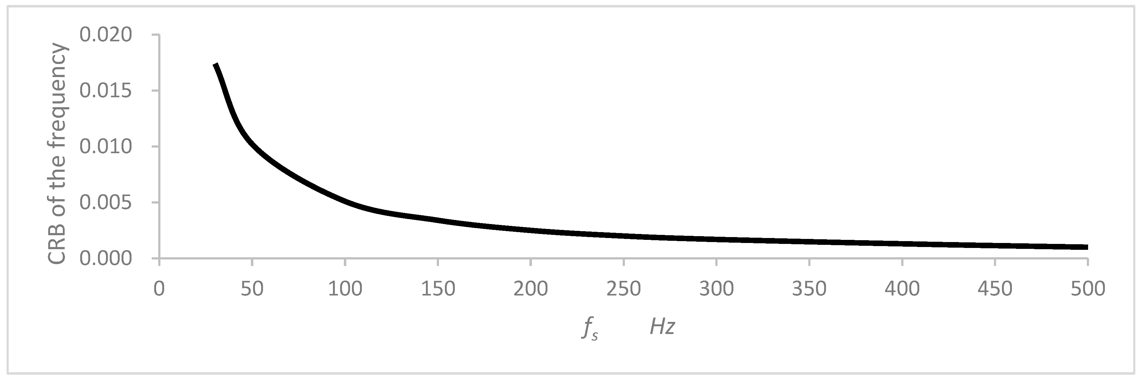
Assuming that a = 1.0$,\mathsf{\beta }=\frac{0.05{\omega }_1}{f_s}$, ${\omega }_1=\frac{62.8}{f_s}(\mathrm{f}=10 \mathrm{H}\mathrm{z})$, $\phi =0$, the noise signal variance $\mathsf{\sigma }=0.2$, and the data sampling length $\mathrm{N}=\mathrm{20,001}$, then $f_s\in \left(30 \mathrm{H}\mathrm{z},500 \mathrm{H}\mathrm{z}\right)$. The Fisher matrix was determined, and subsequently, the CRLB of the frequency was estimated using Equation (36) by substituting these parameters into Equations (23)–(33). The computed results are listed in

Table 1. CRLB of frequency identification corresponding to different sampling frequencies.

$f_s$ (Hz)	30	50	100	150	200	250	300	400	500
CRLB	0.0174	0.0102	0.0051	0.0034	0.0025	0.0020	0.0017	0.0013	0.0010

, with a corresponding visual representation in Figure 2.

The CRLB of a real sinusoidal signal is

$$\mathrm{E}{\left({\widehat{\mathsf{\omega }}}_0-{\mathsf{\omega }}_0\right)}^2\ge \frac{12}{\zeta N(N^2-1)}$$

(37)

where $\zeta$ is the SNR ($\zeta =\frac{a^2}{2{\mathsf{\sigma }}^2}$); N is the length of the data.

The CRLB is the result of normalized sampling frequency, which can be obtained by considering the influence of sampling frequency in the same way as Equation (36).

$$\mathrm{E}{\left({\widehat{\mathsf{\omega }}}_{01}-{\mathsf{\omega }}_{01}\right)}^2\ge \frac{12f_s^2}{\zeta N(N^2-1)}$$

(38)

The free attenuation signal differs significantly from the sinusoidal signal. When the data length of the sinusoidal signal remains constant, and the sampling theorem is met, a lower sampling frequency results in a smaller frequency identification variance. However, simulation results for free attenuation signals indicate that free fading signals’ frequency and time domain resolutions align. As the time domain resolution is enhanced, so is the frequency domain resolution. The simulation results reveal that:

(1)

Elevating the sampling frequency can decrease the lower limit of frequency identification variance. Enhancing the sampling frequency improves the frequency identification accuracy at low sampling frequencies.

(2)

Continuously increasing the sampling frequency does not indefinitely enhance recognition accuracy. When the sampling frequency is 40 times the recognition frequency, further increases in the sampling frequency minimally impact recognition accuracy.

(3)

Free-damping vibration signals differ markedly from sinusoidal signals. A lower sampling frequency yields higher frequency identification accuracy with consistent data length. A higher sampling frequency increases frequency identification accuracy with a sufficiently long signal length. Thus, a higher sampling frequency can be employed for signal acquisition to boost frequency identification accuracy in actual modal tests.

(4)

According to the influence of the sampling frequency of the free-damping vibration signals on the accuracy of frequency identification, a real-time eigen perturbation strategy can be further adopted to adaptively adjust the sampling frequency in real-time modal testing, thereby improving the accuracy of frequency identification [5].

(2)

Influence of damping coefficient on frequency identification accuracy 

Assuming that a = 1.0$,\mathsf{\beta }=\frac{\mathsf{\xi }{\omega }_1}{f_s}$, ${\omega }_1=\frac{62.8}{f_s}(\mathrm{f}=10\mathrm{H}\mathrm{z})$, $\phi =0$, noise signal variance $\mathsf{\sigma }=0.2$, data sampling length $\mathrm{N}=\mathrm{20,001}$, and $f_s=500\mathrm{H}\mathrm{z}$, then $\mathsf{\xi }\in \left(0.01,0.1\right)$. The Fisher matrix was computed, and subsequently, the CRLB of the frequency was determined using Equation (36) by substituting these parameters into Equations (23)–(33).

Table 2. Different damping coefficients correspond to the CRLB.

$\xi$	0.01	0.02	0.03	0.04	0.05	0.06	0.08	0.10
CRLB	8.0465 × 10−6	6.4468 × 10−6	2.1812 × 10−4	5.1882 × 10−4	0.0010	0.0018	0.0042	0.0084

details the outcomes, whereas Figure 3 represents them.

The simulation findings show that the frequency identification error also rises as the signal damping coefficient increases. Hence, in systems with a larger damping coefficient, the impact of this coefficient must be accounted for during system frequency identification.

(3)

Influence of noise on frequency identification accuracy 

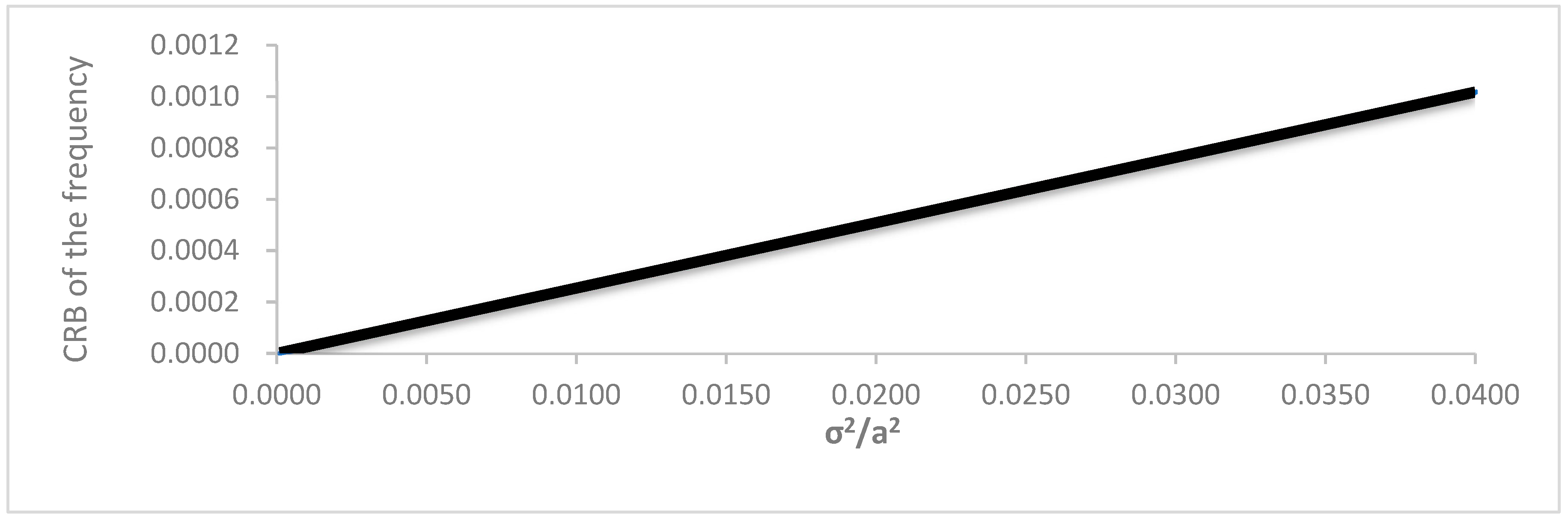
If a = 1.0$,\mathsf{\beta }=\frac{0.05{\omega }_1}{f_s}$, ${\omega }_1=\frac{62.8}{f_s}(\mathrm{f}=10\mathrm{H}\mathrm{z})$, $\phi =0$, data sampling length $\mathrm{N}=\mathrm{20,001}$, and $f_s=500\mathrm{H}\mathrm{z}$, then$\mathsf{\sigma }\in \left(0.01,0.2\right)$. The Fisher matrix was determined, and then the CRLB of the frequency was estimated using Equation (36) by substituting these parameters into Equations (23)–(33). The calculation results are listed in

Table 3. The CRLB of frequency identification at different SNRs.

$\sigma$	0.0100	0.0164	0.0270	0.0347	0.0446	0.0573	0.0736	0.1213	0.2000
${\mathsf{\sigma }}^2/{\mathrm{a}}^2$	0.0001	0.0003	0.0007	0.0012	0.0020	0.0033	0.0054	0.0147	0.0400
SNRs (dB)	30	20	10	5	0	−5	−10	−20	−30
CRLB	2.545 × 10−6	6.844 × 10−6	1.855 × 10−5	3.064 × 10−5	5.062 × 10−5	8.355 × 10−5	1.378 × 10−4	3.744 × 10−4	1.018 × 10−3

, and the graph is shown in Figure 4.

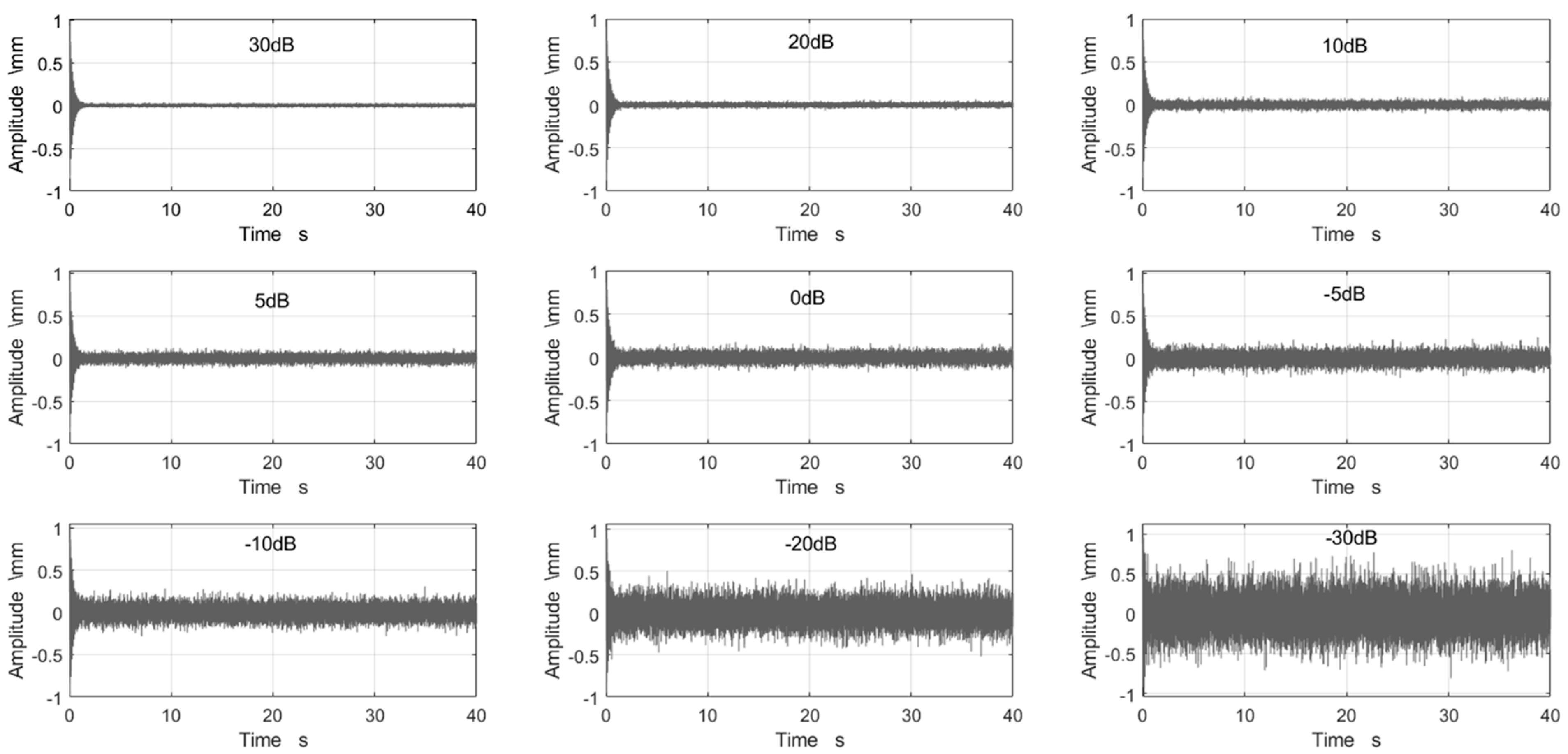
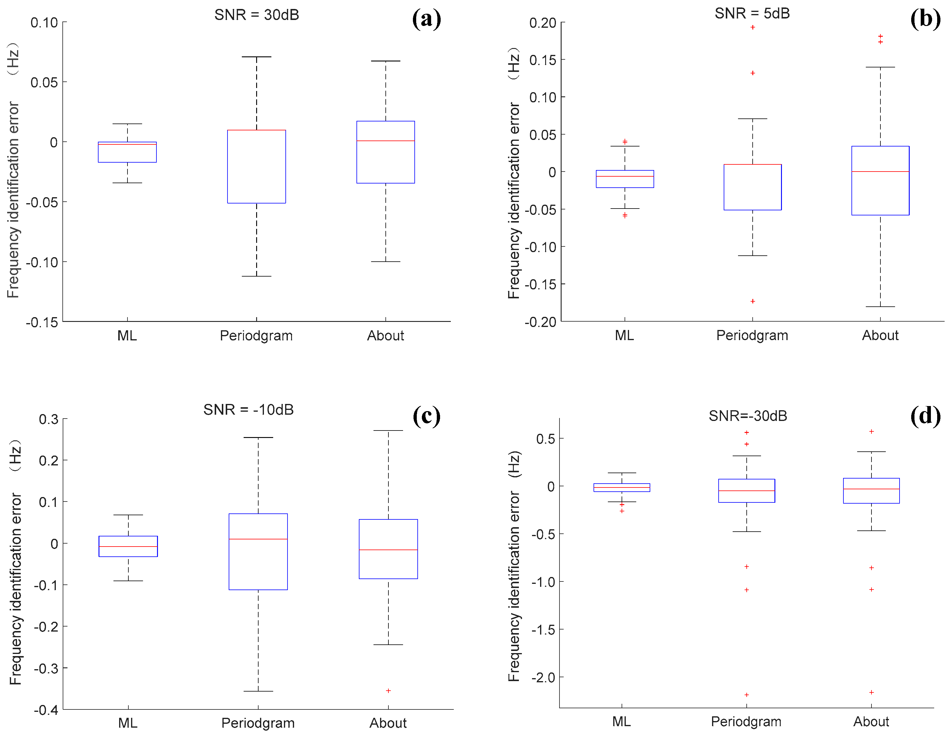
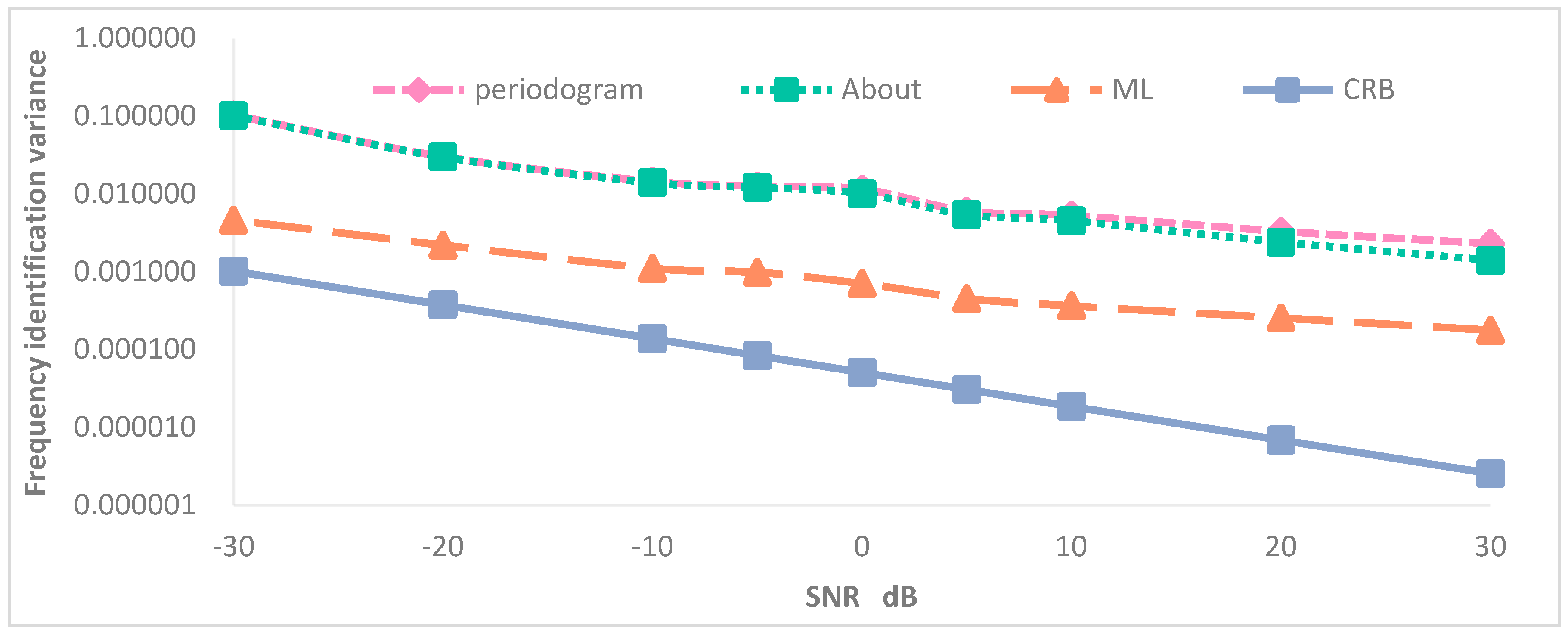
The simulation results indicate that the CRLB of frequency parameter identification is proportional to $\frac{{\mathrm{a}}^2}{{\mathsf{\sigma }}^2}$. As noise increases, the accuracy of frequency identification decreases. Consequently, the initial step in frequency parameter identification should involve signal denoising. Enhancing the SNR can notably enhance the frequency identification accuracy.

(4)

Influence of the phase of the signal on frequency identification accuracy 

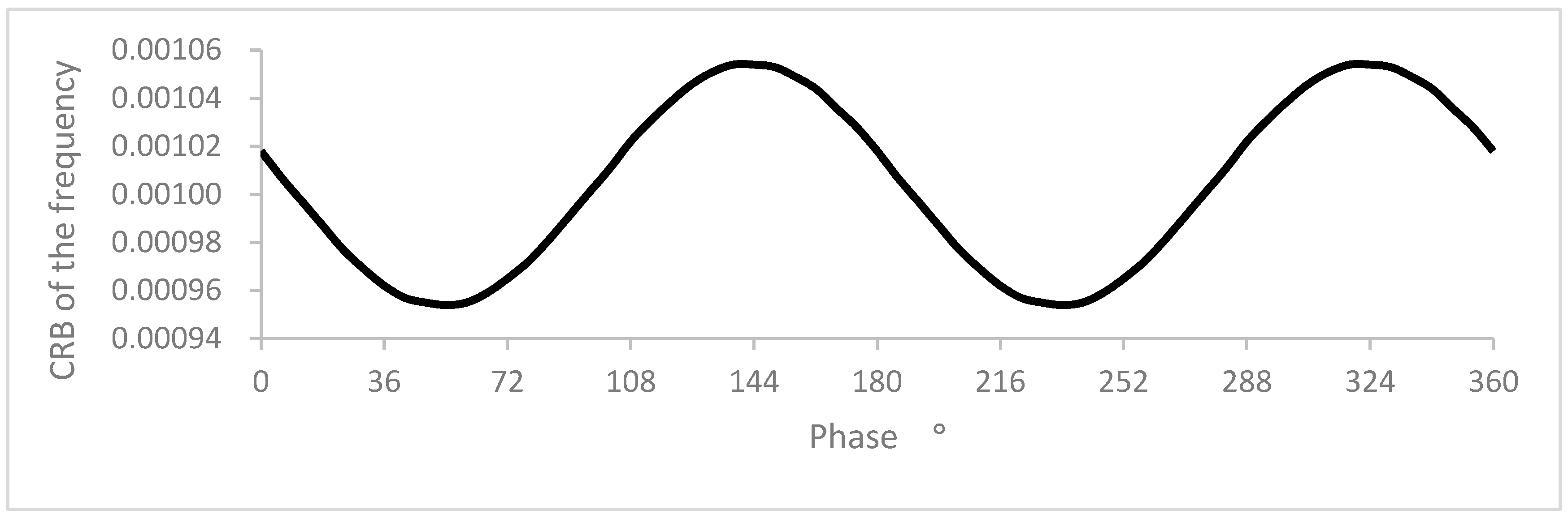
Assuming that a = 1.0$,\mathsf{\beta }=\frac{0.05{\omega }_1}{f_s}$, ${\omega }_1=\frac{62.8}{f_s}(\mathrm{f}=10\mathrm{H}\mathrm{z})$, data sampling length $\mathrm{N}=\mathrm{20,001}$, $f_s=500\mathrm{H}\mathrm{z}$, and$\mathsf{\sigma }=0.2$, then$\phi \in \left(0,360\right)$. By substituting the above parameters into Equations (23)–(33), the Fisher matrix was calculated, and then the CRLB of the frequency was estimated from Equation (36). The calculation results are listed in

Table 4. The CRLB of frequency identification at different phases.

Phase (°)	0	36	54	90	126	144	180	198	360
CRLB	0.00102	0.00096	0.00095	0.00099	0.00105	0.00105	0.00102	0.00099	0.00102

and illustrated in Figure 5.

The simulation results indicate the following: (1) The phase angle significantly affects the lower variance of frequency parameter identification. The variance is lowest when the phase angle is approximately 54° and 234° and highest at approximately 144° and 324°. (2) The difference between the maximum and minimum values of the CRLB is 0.0001 for various phase angles.

Since the phase angle’s influence is less pronounced than the noise, sampling frequency, and damping coefficient, the randomness of excitation in actual sampled signals renders the phase angle uncertain. Consequently, the superposition of free-damping signals with identical frequencies but differing phase angles can lead to the spectral line-splitting phenomenon. This uncertainty can adversely affect the accuracy of frequency identification.

2.3. Algorithm Derivation and Its Methods

Maximum likelihood estimation seeks to estimate parameters based on known observations, without prior knowledge of the unknown quantity under consideration. In applying the maximum likelihood estimation method, the parameters to be estimated are considered constant, though they remain unknown, while the known observation data are treated as random sequences. Let $\mathrm{x}=({\mathrm{x}}_1,{\mathrm{x}}_2,\cdots ,{\mathrm{x}}_{\mathrm{N}})$ represent N observations of random variables and let $\left\{f\left(\mathrm{x}|\mathsf{\theta }\right),\mathsf{\theta }\in \mathsf{\Theta }\right\}$ represent the joint conditional probability density function of observed samples with specific parameters, where θ is the potential range of values. The joint conditional probability density function is as follows:

$$f\left(\theta \right)=f\left(\mathrm{x}|\theta \right){\prod }_{i=1}^{n}f\left(x_i|\theta \right)$$

(39)

Assuming that the joint conditional probability density function exists and is constrained, the maximum likelihood estimation is the estimation value $\widehat{\mathsf{\theta }}$ that optimizes the likelihood function $\left\{\mathrm{f}\left(\mathrm{x}|\mathsf{\theta }\right),\mathsf{\theta }\in \mathsf{\Theta }\right\}$. Given a sampling frequency of 1 Hz, the probability density function for a single-frequency free damping vibration signal is presented as follows:

$$\mathrm{f}\left(\mathrm{x},\mathsf{\theta }\right)=\frac{1}{{\left(2\mathsf{\pi }{\mathsf{\sigma }}^2\right)}^{\frac{\mathrm{N}}{2}}}\mathrm{e}\mathrm{x}\mathrm{p}\left\{-\frac{1}{2{\mathsf{\sigma }}^2}{\sum }_{\mathrm{n}=0}^{\mathrm{N}-1}{\left[\mathrm{x}\left(\mathrm{n}\right)-\mathrm{a}{\mathrm{e}}^{-\mathsf{\beta }n}\mathrm{c}\mathrm{o}\mathrm{s}\left({\omega }_{1}n+\phi \right)\right]}^2\right\}$$

(40)

where $\mathsf{\beta }=\mathsf{\xi }{\omega }_0,{\omega }_1=\sqrt{1-{\mathsf{\xi }}^2}{\mathsf{\omega }}_0$.

When the identification parameter $\widehat{\mathsf{\theta }}$ results in $\mathrm{f}\left(\mathrm{x},\mathsf{\theta }\right)$ achieving its maximum value, this parameter represents the maximum likelihood estimation. Taking the logarithm of f(x,θ) yields the following expression:

$$\ln \left(\mathrm{f}\left(\mathrm{x},\mathsf{\theta }\right)\right)=-\frac{\mathrm{N}}{2}\mathrm{l}\mathrm{n}\left(2\mathsf{\pi }{\mathsf{\sigma }}^2\right)-\frac{1}{2{\mathsf{\sigma }}^2}{\sum }_{\mathrm{n}=0}^{\mathrm{N}-1}{\left[\mathrm{x}\left(\mathrm{n}\right)-\mathrm{a}{\mathrm{e}}^{-\mathsf{\beta }n}\mathrm{c}\mathrm{o}\mathrm{s}\left({\omega }_{1}n+\phi \right)\right]}^2$$

(41)

and

$$\mathrm{L}\left(\mathrm{x},\mathsf{\theta }\right)={\sum }_{\mathrm{n}=0}^{\mathrm{N}-1}{\left[\mathrm{x}\left(\mathrm{n}\right)-\mathrm{a}{\mathrm{e}}^{-\mathsf{\beta }n}\mathrm{c}\mathrm{o}\mathrm{s}\left({\omega }_{1}n+\phi \right)\right]}^2$$

(42)

Expanding Equation (42) yields

$$\mathrm{L}\left(\mathrm{x},\mathsf{\theta }\right)={\sum }_{\mathrm{n}=0}^{\mathrm{N}-1}\left[{\mathrm{x}}^2\left(\mathrm{n}\right)+{\mathrm{a}}^2{\mathrm{e}}^{-2\mathsf{\beta }n}{\mathrm{c}\mathrm{o}\mathrm{s}}^2\left({\omega }_{1}n+\phi \right)-2a\mathrm{x}\left(\mathrm{n}\right){\mathrm{e}}^{-\mathsf{\beta }n}\mathrm{c}\mathrm{o}\mathrm{s}\left({\omega }_{1}n+\phi \right)\right]$$

(43)

By ignoring the known time series, ${\sum }_{\mathrm{n}=0}^{\mathrm{N}-1}{\mathrm{x}}^2\left(\mathrm{n}\right)$, from Equation (43), we can derive

$${\mathrm{L}}_0\left(\mathrm{x},\mathsf{\theta }\right)=\frac{{\mathrm{a}}^2}{4\mathsf{\beta }}-2\mathrm{a}{\sum }_{\mathrm{n}=0}^{\mathrm{N}-1}\mathrm{x}\left(\mathrm{n}\right){\mathrm{e}}^{-\mathsf{\beta }n}\mathrm{c}\mathrm{o}\mathrm{s}\left({\omega }_{1}n+\phi \right)$$

(44)

When a and β are unknown values, then

$${\mathrm{L}}_0\left(\mathrm{x},\mathsf{\omega }\right)={\sum }_{\mathrm{n}=0}^{\mathrm{N}-1}\mathrm{x}\left(\mathrm{n}\right){\mathrm{e}}^{-\mathsf{\beta }n}\mathrm{c}\mathrm{o}\mathrm{s}\left(\omega n+\phi \right)$$

(45)

When the parameter $\widehat{\mathsf{\omega }}$ causes $\mathrm{f}\left(\mathrm{x},{\mathsf{\omega }}_1\right)$ to achieve its maximum, $\ln \left(\mathrm{f}\left(\mathrm{x},\widehat{\mathsf{\omega }}\right)\right)$ reaches its maximum, whereas $\mathrm{L}\left(\mathrm{x},\mathsf{\theta }\right)$ and ${\mathrm{L}}_0\left(\mathrm{x},\mathsf{\theta }\right)$ achieve their minima and ${\mathrm{L}}_0\left(\mathrm{x},{\mathsf{\omega }}_1\right)$ attains its maximum. Maximum likelihood estimation is equivalent to the best square approximation estimation.

Based on Equation (45), ${\mathrm{L}}_0\left(\mathrm{x},\mathsf{\omega }\right)$ has the greatest value when identifying the parameter $\widehat{\mathsf{\omega }}\to {\omega }_1$, where $\widehat{\mathsf{\omega }}$ is the maximum likelihood estimation parameter.

Taking the partial derivative of ${\mathrm{L}}_0\left(\mathrm{x},\mathsf{\omega }\right)$, we can obtain

$$\mathrm{L}\mathrm{x}\left(\mathrm{x},\mathsf{\omega }\right)=\frac{\partial {\mathrm{L}}_0\left(\mathrm{x},\mathsf{\theta }\right)}{\partial \mathsf{\omega }}=-2\mathrm{a}{\sum }_{\mathrm{n}=0}^{\mathrm{N}-1}\mathrm{x}\left(\mathrm{n}\right){\mathrm{n}\mathrm{e}}^{-\mathsf{\beta }n}\mathrm{s}\mathrm{i}\mathrm{n}\left(\omega n+\phi \right)$$

(46)

When Equation (40) attains the maximum value, $\mathrm{L}\mathrm{x}\left(\mathrm{x},\mathsf{\omega }\right)=0$. When $\widehat{\mathsf{\omega }}\to {\omega }_1$, we can obtain

$${\sum }_{\mathrm{n}=0}^{\mathrm{N}-1}\mathrm{x}\left(\mathrm{n}\right){\mathrm{n}\mathrm{e}}^{-\mathsf{\beta }n}\mathrm{s}\mathrm{i}\mathrm{n}\left(\widehat{\mathsf{\omega }}n+\phi \right)=0$$

(47)

Likewise, if $\mathrm{a},\mathsf{\beta },\mathrm{a}\mathrm{n}\mathrm{d}\mathsf{\phi }$ in the parameter$\mathsf{\theta }={\left[\mathrm{a},{\mathsf{\omega }}_1,\mathsf{\beta },\mathsf{\phi }\right]}^{\mathrm{T}}$ are deduced similarly to the parameter ${\mathsf{\omega }}_1$, then

$$\mathrm{L}\mathrm{x}\left(\mathrm{x},\mathrm{a}\right)=\frac{\partial {\mathrm{L}}_0\left(\mathrm{x},\mathsf{\theta }\right)}{\partial \mathrm{a}}=\frac{\mathrm{a}}{2\mathsf{\beta }}-2{\sum }_{\mathrm{n}=0}^{\mathrm{N}-1}\mathrm{x}\left(\mathrm{n}\right){\mathrm{e}}^{-\mathsf{\beta }n}\mathrm{c}\mathrm{o}\mathrm{s}\left({\omega }_{1}n+\phi \right)=0$$

(48)

When $\widehat{\mathrm{a}}\to \mathrm{a}$, then

$$\widehat{\mathrm{a}}=4\mathsf{\beta }{\sum }_{\mathrm{n}=0}^{\mathrm{N}-1}\mathrm{x}\left(\mathrm{n}\right){\mathrm{e}}^{-\mathsf{\beta }n}\mathrm{c}\mathrm{o}\mathrm{s}\left({\omega }_{1}n+\phi \right)$$

(49)

When $\widehat{\mathsf{\beta }}\to \mathsf{\beta }$, the following can be derived:

$${\sum }_{\mathrm{n}=0}^{\mathrm{N}-1}\mathrm{x}\left(\mathrm{n}\right){\mathrm{n}\mathrm{e}}^{-\widehat{\mathsf{\beta }}n}\mathrm{c}\mathrm{o}\mathrm{s}\left({\omega }_{1}n+\phi \right)\approx \frac{a}{8{\widehat{\beta }}^2}$$

(50)

The following can be obtained from Equations (49) and (50):

$$\widehat{\mathsf{\beta }}=\frac{{\sum }_{\mathrm{n}=0}^{\mathrm{N}-1}\mathrm{x}\left(\mathrm{n}\right){\mathrm{e}}^{-\mathsf{\beta }n}\mathrm{c}\mathrm{o}\mathrm{s}\left(\widehat{\mathsf{\omega }}n+\phi \right)}{2{\sum }_{\mathrm{n}=0}^{\mathrm{N}-1}\mathrm{x}\left(\mathrm{n}\right){\mathrm{n}\mathrm{e}}^{-\mathsf{\beta }n}\mathrm{c}\mathrm{o}\mathrm{s}\left(\widehat{\mathsf{\omega }}n+\phi \right)}$$

(51)

When $\widehat{\mathsf{\phi }}\to \mathsf{\phi }$, then

$$\widehat{\phi }={-\tan }^{-1}\frac{{\sum }_{\mathrm{n}=0}^{\mathrm{N}-1}\mathrm{x}\left(\mathrm{n}\right){\mathrm{e}}^{-\mathsf{\beta }n}\mathrm{s}\mathrm{i}\mathrm{n}\left(\widehat{\mathsf{\omega }}n\right)}{{\sum }_{\mathrm{n}=0}^{\mathrm{N}-1}\mathrm{x}\left(\mathrm{n}\right){\mathrm{e}}^{-\mathsf{\beta }n}\mathrm{c}\mathrm{o}\mathrm{s}\left(\widehat{\mathsf{\omega }}n\right)}$$

(52)

Based on the above deduction, the frequency identification of a free-damping vibration signal can be categorized into the following steps:

(1)

The frequency and damping coefficient parameters are initially estimated using the self-power spectrum;

(2)

The initial estimated frequency and damping coefficient parameters are substituted into Equation (52), and the corresponding calculations is performed to obtain phase angle parameters;

(3)

The initial estimated damping coefficient and phase angle estimation parameter are substituted into Equation (45), and the new estimated frequency corresponds to its maximum value;

(4)

The iteration is repeated from the second to the third step to continuously improve recognition accuracy.

Figure 6 depicts the flowchart of frequency parameter identification using the maximum likelihood method.

3. Results

3.1. Simulation Signal Model

For the simulation calculation model (Equation (10)), assuming that a = 1.0$,\mathsf{\beta }=\frac{0.05{\omega }_1}{f_s}$, ${\omega }_1=\frac{62.8}{f_s}(\mathrm{f}=10\mathrm{H}\mathrm{z})$, $\phi =0$, data sampling length $\mathrm{N}=\mathrm{20,001}$, $f_s=500\mathrm{H}\mathrm{z}$, and $\mathsf{\sigma }\in \left(0.01,0.2\right)$, the SNR ranges between 30 and −30 dB. Figure 7 illustrates the time domain curves at different SNRs.

3.2. Error Analysis

A rough estimation of the damping coefficient and frequency is required during the estimation process using the maximum likelihood algorithm. The rough estimation values are simulated within a specific error range to evaluate the impact of the accuracy of these rough estimates on frequency estimation. Assuming that the error in the rough estimate of the frequency ranges from −20% to 20%, meaning the rough estimate frequency lies between 8 and 12 Hz, the effect on recognition results is presented in

Table 5. Identification results of the four iterations for initial estimation of different frequencies (Hz).

Initial Estimation	8.0	8.4	9.0	9.6	10.0	10.4	11.0	11.4	12.0
Results of one iteration	9.702	9.728	9.790	9.894	9.990	10.080	10.180	10.222	10.264
Second iteration result	9.848	9.862	9.892	9.944	9.992	10.040	10.080	10.104	10.124
Triple iteration result	9.920	9.926	9.940	9.964	9.988	10.010	10.030	10.044	10.054
Results of four iterations	9.974	9.976	9.978	9.986	9.990	9.994	10.000	10.002	10.006

. Based on the simulation findings, when the rough frequency estimate ranges from −20% to 20%, the recognition error can be diminished to less than 0.26% after four iterations. Consequently, the maximum likelihood frequency estimation algorithm is not significantly influenced by the initial estimate and can rapidly converge to the actual frequency value through numerous iterations.

Similarly, the impact of the initial estimate of the damping coefficient on frequency identification accuracy is also simulated. Assuming that the initial error in estimating the damping coefficient ranges from −50% to 50%, meaning the damping coefficient varies between 0.025 and 0.075, the maximum likelihood method estimates the frequency for different damping coefficients. These simulation results are documented in

Table 6. Frequency identification results of initial estimation of different damping coefficients.

Initial Estimation	0.025	0.035	0.040	0.045	0.050	0.055	0.060	0.070	0.075
Frequency estimation (Hz)	10.007	10.008	9.999	9.997	9.993	9.989	9.987	9.977	9.973

. When the damping coefficient ranges from −50% to 50%, the most considerable discrepancy in identification frequency is only 0.034 Hz, and the maximum error in frequency identification is 0.34%. Hence, in the practical algorithm, the initial estimate of the damping coefficient is determined using the power spectrum half-power bandwidth method, and the damping coefficient does not require iterative calculations. The maximum likelihood frequency estimation algorithm is not sensitive to changes in the damping coefficient.

The identification errors in the initial amplitude A and damping coefficient ξ of a free damping signal exert minimal influence on frequency parameter identification. However, the phase angle significantly impacts frequency parameter identification. Therefore, only the phase angle requires iterative solutions when employing the maximum likelihood method for iterative identification. The identification results for the initial amplitude and damping coefficient within a specific range do not compromise the accuracy of frequency parameter identification.

3.3. Comparative Analysis of Recognition Results of Different Methods

The frequency parameters of freely attenuated vibration signals at varying SNRs were identified using the periodogram, dichotomy interpolation, and maximum likelihood methods. One hundred groups of random simulation identifications were conducted for signals with the same SNR. The frequency identification error is depicted in Figure 8. The maximum likelihood method significantly enhanced the identification accuracy. This improvement was particularly noticeable when the SNR is low, leading to a notable increase in the frequency recognition correctness rate.

The variances in recognition results for the three algorithms were calculated based on the recognition results for each group of signals with identical SNRs. The CRLB bounds for these results were also computed under the respective conditions.

Table 7. Frequency parameter identification variance of different identification methods.

$\sigma$	0.0100	0.0164	0.0270	0.0347	0.0446	0.0573	0.0736	0.1213	0.2000
SNR dB	30	20	10	5	0	−5	−10	−20	−30
perodogram	0.0023	0.0033	0.0053	0.0060	0.0115	0.0126	0.0145	0.0301	0.1032
About	0.0014	0.0024	0.0045	0.0054	0.0101	0.0121	0.0139	0.0297	0.1013
ML	1.771 × 10−4	2.548 × 10−4	3.638 × 10−4	4.528 × 10−4	7.058 × 10−4	9.818 × 10−4	1.100 × 10−3	2.200 × 10−3	4.600 × 10−3
CRLB	2.545 × 10−6	6.844 × 10−6	1.855 × 10−5	3.064 × 10−5	5.062 × 10−5	8.355 × 10−5	1.378 × 10−4	3.744 × 10−4	1.018 × 10−3

lists the findings, whereas Figure 9 displays the relationship curves between frequency identification variance and signal-to-noise ratio for the various identification methods.

From the error analysis, several conclusions can be drawn:

• The recognition accuracy of the dichotomy interpolation method marginally surpasses that of the periodogram method.
• The maximum likelihood method’s recognition accuracy is significantly superior to the periodogram and the dichotomy interpolation methods across all SNR conditions. Approximately an order of magnitude enhances its accuracy.
• As the SNR decreases, the variance in the maximum likelihood recognition approaches the lower bound of the CRLB variance, indicating that the maximum likelihood recognition algorithm is highly noise-resistant.
• Enhancing the frequency resolution and the number of data calculation bits of the maximum likelihood method can further boost recognition accuracy.
• The maximum likelihood method requires an iterative solution, making its computational demand considerably greater than that of the periodogram method.

4. Conclusions

The study focuses on the free-damping signal mixed with white noise to enhance the frequency parameter identification accuracy of the structural response signal under ambient excitation. The primary conclusions are:

1.

The free-damping vibration signal possesses limited energy. As $\mathrm{t}$ approaches infinity, $\tilde{\mathrm{a}}$ approaches zero. With an extended sampling time, the SNR decreases; when the sample time T approaches infinity, the SNR $\tilde{\mathsf{\varsigma }}$ approaches zero.

2.

Based on the CRBL for the free damping signal and the simulation results, the following observations were made:

(a)

An increase in the sampling frequency reduces the lower bound of frequency identification variance. Specifically, when the sampling frequency is low, raising it improves frequency identification accuracy. However, increasing the sampling frequency does not always enhance recognition accuracy. After the sampling frequency reaches 40 times the recognition frequency, further increases in the sampling frequency minimally affect the recognition accuracy.

(b)

A higher signal damping coefficient results in greater frequency identification error. For systems with large damping coefficients, the effect of the damping coefficient should be factored in during system frequency identification.

(c)

The CRB for frequency parameter identification is proportional to $\frac{{\mathrm{a}}^2}{{\mathsf{\sigma }}^2}$. Increased noise leads to decreased frequency identification accuracy.

(d)

The influence of the phase angle is less significant than the noise, sampling frequency, and damping coefficient. However, phase angles can vary due to the unpredictability of excitation in actual sampled signals. Consequently, the superposition of free-damping signals with identical frequencies but differing phase angles can split spectral lines. This variability can reduce the accuracy of actual frequency identification.

3.

Compared to the periodogram method and the dichotomy interpolation method, the recognition accuracy of the maximum likelihood method is substantially superior under various SNR conditions, improving accuracy by roughly an order of magnitude.

References

1. Masi, A.; Santarsiero, G.; Chiauzzi, L. Development of a seismic risk mitigation methodology for public buildings applied to the hospitals of Basilicata region (Southern Italy). Soil Dyn. Earthq. Eng. 2014, 65, 30–42. [Google Scholar] [CrossRef]
2. Guo, Y.; Guo, S. Structural Damage Detection And Image Based On The Zero Migration Record Of The Synthetical Pseudo-Spectrum. Eng. Mech. 2014, 31, 29–36. [Google Scholar] [CrossRef]
3. Gromyko, P.V.; Fedin, K.V.; Seleznev, V.S.; Kolesnikov, Y.I.; Ngomayezwe, L. Monitoring of the hydraulic units operation of the Sayano-Shushenskaya hydroelectric power plant using remote seismic observations. Earthq. Eng. Struct. Dyn. 2023, 52, 335–349. [Google Scholar] [CrossRef]
4. Bhowmik, B.; Tripura, T.; Hazra, B.; Pakrashi, V. Robust linear and nonlinear structural damage detection using recursive canonical correlation analysis. Mech. Syst. Signal Process. 2019, 136, 106499. [Google Scholar] [CrossRef]
5. Bhowmik, B.; Tripura, T.; Hazra, B.; Pakrashi, V. Real time structural modal identification using recursive canonical correlation analysis and application towards online structural damage detection. J. Sound Vib. 2019, 468, 115101. [Google Scholar] [CrossRef]
6. Yuan, P.-P.; Zhang, J.; Feng, J.-Q.; Wang, H.-H.; Ren, W.-X.; Wang, C. An improved time-frequency analysis method for structural instantaneous frequency identification based on generalized S-transform and synchroextracting transform. Eng. Struct. 2022, 252, 113657. [Google Scholar] [CrossRef]
7. Civera, M.; Calamai, G.; Zanotti Fragonara, L. Experimental modal analysis of structural systems by using the fast relaxed vector fitting method. Struct. Control Health Monit. 2021, 28, e2695. [Google Scholar] [CrossRef]
8. Xu, G.; Guo, T.; Li, A.; Zhang, R.; Zhu, R.; Liu, F. Influence of ambient temperature on seismic performance of elastomeric isolation structural system. Structures 2023, 55, 1763–1773. [Google Scholar] [CrossRef]
9. Çetindemir, O.; Zülfikar, A.C.; Apaydın, N.M. Dynamic Modal Identification of a Long-Span Suspension Bridge Using Measured Acceleration Data during a Storm. J. Struct. Eng. 2023, 149, 11982. [Google Scholar] [CrossRef]
10. MacLeod, E.; Arjomandi, K. Dynamic bridge weigh-in-motion using estimated modal parameters from ambient vibration tests. Eng. Struct. 2023, 289, 116254. [Google Scholar] [CrossRef]
11. Yi, Q.; Wilcox, P.; Hughes, R. Modelling and evaluation of carbon fibre composite structures using high-frequency eddy current imaging. Compos. Part B Eng. 2023, 248, 110343. [Google Scholar] [CrossRef]
12. Khademi, P.; Mousavi, M.; Dackermann, U.; Gandomi, A.H. Time–frequency analysis of ultrasonic signals for quality assessment of bonded concrete. Constr. Build. Mater. 2023, 403, 133062. [Google Scholar] [CrossRef]
13. He, W.; Lai, W.W.-L.; Sui, X.; Giannopoulos, A. Delamination characterization in thin asphalt pavement structure using dispersive GPR data. Constr. Build. Mater. 2023, 402, 132834. [Google Scholar] [CrossRef]
14. Damadipour, M.; Tarinejad, R. Structural system identification based on combining weighted transmissibility and wavelet transform. Struct. Control Health Monit. 2021, 29, e2868. [Google Scholar] [CrossRef]
15. Ahi, M.; Ahmadian, H. Nonlinear model updating of frictional structures through frequency-energy analysis. Nonlinear Dy-Namics 2022, 110, 95–116. [Google Scholar] [CrossRef]
16. Hou, J.; Cao, S.; Hu, H.; Zhou, Z.; Wan, C.; Noori, M.; Li, P.; Luo, Y. Vortex-Induced Vibration Recognition for Long-Span Bridges Based on Transfer Component Analysis. Buildings 2023, 13, 2012. [Google Scholar] [CrossRef]
17. Ding, Z.; Li, J.; Hao, H. Non-probabilistic method to consider uncertainties in structural damage identification based on Hybrid Jaya and Tree Seeds Algorithm. Eng. Struct. 2020, 220, 110925. [Google Scholar] [CrossRef]
18. Sadeghi, F.; Yu, Y.; Zhu, X.; Li, J. Damage identification of steel-concrete composite beams based on modal strain energy changes through general regression neural network. Eng. Struct. 2021, 244, 112824. [Google Scholar] [CrossRef]
19. Zhao, B.; Lei, D.; Fu, J.; Yang, L.; Xu, W. Experimental study on micro-damage identification in reinforced concrete beam with wavelet packet and DIC method. Constr. Build. Mater. 2019, 210, 338–346. [Google Scholar] [CrossRef]
20. Kato, T. Perturbation Theory for Linear Operators; Springer Science & Business Media: Berlin/Heidelberg, Germany, 2013; Volume 132, p. 132. [Google Scholar]
21. Wang, H.; Barone, G.; Smith, A. A novel multi-level data fusion and anomaly detection approach for infrastructure damage identification and localisation. Eng. Struct. 2023, 292, 116473. [Google Scholar] [CrossRef]
22. Soleymani, A.; Jahangir, H.; Rashidi, M.; Mojtahedi, F.F.; Bahrami, M.; Javanmardi, A. Damage Identification in Reinforced Concrete Beams Using Wavelet Transform of Modal Excitation Responses. Buildings 2023, 13, 1955. [Google Scholar] [CrossRef]
23. Eiras, J.N.; Payan, C.; Rakotonarivo, S.; Garnier, V. Experimental modal analysis and finite element model updating for structural health monitoring of reinforced concrete radioactive waste packages. Constr. Build. Mater. 2018, 180, 531–543. [Google Scholar] [CrossRef]
24. Feng, D.; Feng, M.Q. Computer vision for SHM of civil infrastructure: From dynamic response measurement to damage detection—A review. Eng. Struct. 2018, 156, 105–117. [Google Scholar] [CrossRef]
25. Yang, C. Study on Frequency Estimators under Noise Environment. Ph.D. Thesis, South China University of Technology, Guangzhou, China, 2010. [Google Scholar]
26. Cao, Y. Research on Frequency Estimator for a Noisy Real Sinusoid. Ph.D. Thesis, South China University of Technology, Guangzhou, China, 2012. [Google Scholar]
27. Xin, Y.; Hao, H.; Li, J.; Wang, Z.-C.; Wan, H.-P.; Ren, W.-X. Bayesian based nonlinear model updating using instantaneous characteristics of structural dynamic responses. Eng. Struct. 2019, 183, 459–474. [Google Scholar] [CrossRef]
28. Aboutanios, E.; Mulgrew, B. Iterative frequency estimation by interpolation on Fourier coefficients. IEEE Trans. Signal Process. 2005, 53, 1237–1242. [Google Scholar] [CrossRef]
29. Umesh, S.; Tufts, D. Estimation of parameters of exponentially damped sinusoids using fast maximum likelihood estimation with application to NMR spectroscopy data. IEEE Trans. Signal Process. 1996, 44, 2245–2259. [Google Scholar] [CrossRef]
30. Zhang, J.; Swain, A.K.; Nguang, S.K. Parameter estimation of exponentially damped sinusoids based on state-space model. J. Jilin Univ. 2019, 49, 2083–2088. [Google Scholar]
31. Chen, G.-W.; Omenzetter, P.; Beskhyroun, S. Operational modal analysis of an eleven-span concrete bridge subjected to weak ambient excitations. Eng. Struct. 2017, 151, 839–860. [Google Scholar] [CrossRef]
32. Gentile, C.; Saisi, A. Operational modal testing of historic structures at different levels of excitation. Constr. Build. Mater. 2013, 48, 1273–1285. [Google Scholar] [CrossRef]
33. Giordano, E.; Mendes, N.; Masciotta, M.G.; Clementi, F.; Sadeghi, N.H.; Silva, R.A.; Oliveira, D.V. Expeditious damage index for arched structures based on dynamic identification testing. Constr. Build. Mater. 2020, 265, 120236. [Google Scholar] [CrossRef]
34. Kay, S.M. Fundamentals of Statistical Signal Processing: Estimation Theory; Prentice Hall Ptr: Upper Saddle River, NJ, USA, 1993. [Google Scholar]
Figure 1. The random excitation response signal of single−degree−of−freedom system: (a) time domain signal; (b) power spectral density(psd) and the frequency.
Buildings 14 00198 g001
Figure 2. The relation between the CRLB and sampling frequency.
Buildings 14 00198 g002
Figure 3. The relation between CRLB and damping coefficient.
Buildings 14 00198 g003
Figure 4. The relation between CRLB and SNR.
Buildings 14 00198 g004
Figure 5. The relation between CRLB and phase.
Buildings 14 00198 g005
Figure 6. Flowchart of maximum likelihood algorithm.
Buildings 14 00198 g006
Figure 7. Time domain curves of different SNRs.
Buildings 14 00198 g007
Figure 8. The box plot of the frequency identification error at different SNRs: (a) SNR = 30 dB; (b) SNR = 5 dB; (c) SNR = −10 dB; (d) SNR = −30 dB.The red dots represent discrete data points outside the interval.
Buildings 14 00198 g008
Figure 9. Relation of frequency identification variance and SNRs of different identification methods.
Buildings 14 00198 g009