Abstract
The development of digital twins leads to the pathway toward intelligent buildings. Today, the overwhelming rate of data in buildings carries a high amount of information that can provide an opportunity for a digital representation of the buildings and energy optimization strategies in the Heating, Ventilation, and Air Conditioning (HVAC) systems. To implement a successful energy management strategy in a building, a data-driven approach should accurately forecast the HVAC features, in particular the indoor temperatures. Accurate predictions not only increase thermal comfort levels, but also play a crucial role in saving energy consumption. This study aims to investigate the capabilities of data-driven approaches and the development of a model for predicting indoor temperatures. A case study of an educational building is considered to forecast indoor temperatures using machine learning and deep learning algorithms. The algorithms’ performance is evaluated and compared. The important model parameters are sorted out before choosing the best architecture. Considering real data, prediction models are created for indoor temperatures. The results reveal that all the investigated models are successful in predicting indoor temperatures. Hence, the proposed deep neural network model obtained the highest accuracy with an average RMSE of 0.16 °C, which renders it the best candidate for the development of a digital twin.
1. Introduction
The world’s energy consumption has significantly increased during the past few decades. According to the estimates from the International Energy Agency, over two decades, primary energy demand has grown by 49%, and emissions have seen a 43% increase, with an average increase of 2% and 1.8%, respectively, each year [1]. A relationship between global warming, climate change, rising pollution, and the expansion in global energy consumption has revealed that reducing energy consumption can impact all the mentioned issues positively. Reducing global energy consumption is a subject worthy of more research and analysis because global population growth is anticipated to increase in the upcoming years, and global energy demands are expected to keep growing.
One of the critical energy consumers in today’s world is the building sector. Building energy consumption has risen to the level of transportation and industry over the last decades as a result of population growth, improved building amenities, and comfort levels, plus increasing time spent in buildings and the spread of building services, particularly heating, ventilation, and air conditioning (HVAC) systems [2].
In Canada, buildings account for 30% of the total energy consumption, and HVAC systems consist of a large portion of it in residential and non-residential buildings [3]. HVAC systems with 59% of total energy consumption account for the largest share of energy use in commercial and institutional buildings in Canada [3].
Optimizing the HVAC energy efficiency benefits the environment and the economy, and implementing proper operational and management strategies is crucial for achieving the best level of energy consumption in buildings. Improving control strategies in HVAC systems through data-driven modeling and prediction techniques has the potential to reduce the overall energy consumption in buildings. Since today people spend most of their time inside buildings, their comfort level must be maintained. Therefore, a key concern in the field of energy management is how to optimize energy consumption without sacrificing thermal comfort level. Indoor temperature predictions can be an efficient measure and effective strategy to optimize the HVAC system [3] while maintaining the occupants’ comfort level.
Incorporating temperature predictions within a Digital Twin HVAC system offers significant advantages in terms of optimizing HVAC system operation. By integrating forecasted temperature conditions, the system gains the ability to proactively adapt its cooling and heating operations. This proactive approach is made possible by leveraging temperature forecasting models that consider variables such as weather patterns and building HVAC characteristics. The system can then make informed decisions regarding the optimal allocation of resources to maintain the desired indoor temperature, ensuring occupant comfort while minimizing energy consumption.
Furthermore, the integration of temperature predictions facilitates the optimization of scheduling within the Digital Twin HVAC system. By considering the anticipated future temperature conditions, the system can strategically activate and deactivate HVAC operations. This approach prevents unnecessary energy consumption during the periods of low occupancy or when temperature adjustments are not required. By aligning the timing of HVAC system operations with forecasted temperature needs, the Digital Twin HVAC system could achieve a higher level of energy efficiency and reduce energy consumption.
Traditionally physical or semi-physical models have been employed to model and predict indoor temperature, but these models’ input parameters are often based on particular building attributes and occupant activity, which are not always easily accessible [4,5,6,7].
Nowadays, modern buildings can negotiate settings that are continually changing because of the interactive and adaptive nature of the buildings, their components, and the surrounding environment. Advanced sensor technologies in buildings are increasingly more capable of inferring valuable information about the building’s properties, outdoor weather conditions (such as temperature, wind, and solar radiation), and occupant behavior (e.g., temperature set points, level). Massive and diverse datasets regarding every aspect of building operations are produced by the continuous communications between smart hubs, sensors within buildings, smart meters, and equipment. For data processing and real-time decision-making, these massive datasets require increasingly automated and adaptable methods to optimize building operations. Therefore, many researchers over the last decade have studied data-driven models to predict indoor temperatures, heating or cooling load, and energy consumption levels.
The majority of data-driven models in the early 2000s were statistical models such as ARIMA (Auto-Regressive Integrated Moving Average) [8]. Common machine learning (ML) algorithms, such as SVR (Support Vector Regression) [9], Random Forest [10], XGBoost [11], etc., have also been widely investigated. Due to the simplicity of the nonlinear parameters included, the minimal demands on feature engineering, and the capacity to handle interactions among nonlinear features, neural networks (NN) have also been increasingly popular in the indoor temperature predictions and energy optimization [12,13].
Both academic scholars and building industry professionals have generally acknowledged predictive modeling as a useful technique to support building design and control. Predictive modeling extracts patterns seen in historical datasets through mathematical methods seeking to predict future events. The building industry has a chance to employ predictive algorithms to lower failure rates, maintenance expenses, and energy consumption while enhancing occupant thermal comfort.
This research investigates suitable data-driven models to predict indoor temperatures toward building a Digital Twin HVAC system. The accuracy of the models was compared through the prediction of the indoor temperature of seven different zones—six classrooms and one office area. The preprocessing and modeling procedure is presented through the use of five-year real operational data collected from the NE01 building at the British Columbia Institute of Technology, located in the city of Burnaby, BC, Canada. Finally, the results were evaluated to propose the most efficient and accurate model for the prediction of indoor temperatures.
2. Related Studies
Indoor temperature prediction is one of the important methods for determining thermal comfort levels in buildings and identifying energy-saving potential, particularly when it is used to develop HVAC system control strategies. Over the last decade, different studies have been carried out to model HVAC systems and simulate indoor temperatures.
Classically, to model and optimize HVAC systems, physics-based models have been widely developed to express the complex laws of physics, energy, heat transfer, and thermodynamics in buildings. Most of these models were built for the purpose of systems control and energy efficiency. In this regard, Nassif et al. [14,15,16] developed a supervisory control strategy based on a simplified physics-based model for a Variable Air Volume (VAV) system to optimize the multi-zone HVAC system. As HVAC systems become more complex, non-linear, and large-scale involving numerous constraints and variables, developing physics-based models for buildings energy management becomes more challenging [17]. In order to generate accurate physics-based models, high-order complex models are often used. The latter are computationally expensive while reducing the model order leads to an increase in prediction error [18]. Furthermore, high computational time makes complex models difficult to apply and implement in real-time applications [19]. Thus, the produced physics-based models are usually deterministic, requiring multiple assumptions and simplifications on their parameters, rendering models less applicable to represent and interfere with the buildings’ daily operations.
To overcome the shortfalls of classical physics-based models, many data-driven approaches have been developed in recent years, and many studies have concentrated on developing predictive models based on data mining techniques. Data-driven models also referred to as “black box” models in artificial intelligence are built straight from data by an algorithm, which cannot be easily comprehended nor interpreted to explain the integration of variables to produce predictions.
Therefore, in recent years, researchers working on modeling HVAC systems have focused on indoor temperature predictions using artificial intelligence algorithms. These algorithms employ various approaches to build models, such as machine learning (ML) tree-based models and deep learning (DL) neural networks.
Tree-based machine learning models are constructed by recursively dividing the considered observations following specific criteria. These criteria are created by comparing all possible splits in the data and selecting the one that provides the highest mean squared error (MSE) reduction in the variance of child nodes. Tree-based ensemble methods enhance performance and create stronger predictive models by combining multiple decision tree predictors. Several studies [20,21,22] have examined the effectiveness of ensemble methods, including Random Forest and Extra Trees, in forecasting time series datasets and specifically HVAC systems.
On the other hand, a deep learning strategy is based on artificial neural networks (ANN). It involves scanning the data with an algorithm to find features that correlate, then combining those features to facilitate rapid learning [23]. These algorithms have the capacity to learn on their own and generate outputs that are independent of their inputs. They are also capable of accomplishing several tasks in parallel, without impacting the system’s performance. Studies show that systems with the ANN modeling approach can handle the internal [24] and external [25] disturbances that impact the modeling process. In addition, researchers have developed strong numerical foundations that enables ANN to handle real-time events because they can learn from examples and apply them when a comparable situation occurs [26,27]. In order to model indoor temperatures, different studies [28,29,30,31,32,33] developed several simple to advanced models with different scenarios, and all discovered that ANN models provided an acceptable accuracy in temperature predictions. However, the literature on artificial neural network (ANN) modeling for buildings primarily focuses on residential buildings and dedicated labs. Researchers in this field often utilize a limited amount of data, typically centered around a single zone within the building, which can impact the comprehensiveness of their findings. Furthermore, the selection of input variables and the preprocessing phase are commonly overlooked, leaving gaps in understanding the methodology employed.
Thomas et al. [28] investigated two types of buildings to develop ANN models for indoor temperature prediction. The first one was a small experimental building, with a total data collection period of 624 h. The second building was a factory building, and the studied area was a laboratory room, with a total data collection of 140 h. Mirzaei et al. [29] presented a simplified model that uses artificial neural network (ANN) techniques to establish a correlation between weather parameters and indoor thermal conditions in residential buildings. The study included a measurement campaign in 55 residential buildings in Montreal. The model incorporates neighborhood-specific parameters, building characteristics, and occupant behavior. Fewer works considered educational buildings to develop ANN models and forecast indoor temperatures. Temperature management and optimization of the thermal conditions in educational buildings is a crucial aspect that significantly impacts the learning environment and students’ well-being. Educational buildings have unique specifications and requirements such as the existence of different areas (e.g., classrooms, offices), the occupancy density and the variety of HVAC features involved in providing a comfortable and productive learning environment. As an example of work carried out in an educational building, Atoue et al. [30] studied office areas of an old school building. The model was developed based on indoor and outdoor temperatures and humidity as well as solar radiation; in addition, collected data from two summer months were used for this study.
In buildings modeled using data-driven techniques, investigations usually consider a single zone area [28,31] and rarely include multiple zones. Afroz et al. [32] evaluated the performance of single-zone and multi-zone indoor temperature prediction models using different combinations of training datasets and inputs. The studied area was concentrated on the second floor of a library building and the data were colected for a few seasons, from summer to winter.
The collected data for the ANN modeling found in the literature were frequently extremely brief, ranging from a few days [10] to a few months [34]. It is well known that ANN performs better when trained on large datasets and that small dataset can significantly limit ANN performance [35]. In fact, small training and test datasets can lead to generalization problems because daily fluctuation of the indoor temperature is insignificant. Therefore, it is essential to look closely at “low” prediction errors; for example, an average RMSE of 0.8 °C might already be too high in comparison to the average daily variance.
The selection of input variables is a crucial subject of investigation in the process of creating models. The input variables and the performance of artificial neural network (ANN) models from different studies [28,29,36] show that researchers often employ input variables without a clear explanation of systematic rationale behind their selection. Moreover, the majority of the studies employing historical data for the purpose of forecasting future interior temperatures have generally failed to provide explicit explanations regarding the preprocessing steps involved [31,32,37,38].
To conclude, it was noticed that there is a lack of comprehensive research exploring the use of deep learning methods for predicting indoor temperatures in educational buildings while considered multiple zones, expanded data collection over many years and detailed data preparation and processing. The research gaps of previous studies can be summarized in the following aspects:
- Limited research exists on the application of deep learning for indoor temperature prediction in educational buildings.
- Consideration of single-zone predictions versus multiple-zone ones.
- Lack of explicit explanations of data preprocessing.
- Extremely brief training periods for ANN models.
The overarching goal of this research is to create a model that would be used to build a digital twin for optimization of the HVAC system operation. The accurate prediction of indoor temperatures is required to achieve this goal. The primary objective of this paper is to select a suitable algorithm to accurately predict indoor temperatures. The secondary objectives are the following:
- To compare the performance and scalability potential of machine learning versus deep learning algorithms to predict indoor temperatures.
- To investigate the system parameters and select the best set of input parameters for model development.
3. Methodology
To achieve the objectives listed above, this research uses a case study HVAC system serving a group of classrooms and an office at the British Columbia Institute of Technology (BCIT). The research consists of four main parts to develop prediction models: data collection and preparation, feature selection and extraction, model development, and performance evaluation.
3.1. Data Collection and Preparation
The data for this study are provided by the Building Management System (BMS) of the British Columbia Institute of Technology. The BMS centralizes building management operations and collects real-time sensor and equipment parameters data.
The raw data that have been collected and archived over the last few years are available and accessible for the institute researchers. Building meaningful features and datasets involves several phases, including data cleaning and transformation.
Several parameters require preprocessing to increase the quality of the data. The database in this study is based on a time series. To reduce the error produced by time delay and system error, the original data were aggregated to 15 min interval data by resampling and filling in missing parameters’ data, well-thought-out in the time intervals.
3.2. Feature Selection and Extraction
The intended purpose of feature selection and extraction is to explore options to improve performance by selecting or extracting features from the existing datasets.
The selection of parameters is based on two approaches. The first approach is based on domain knowledge, and the second approach relies on statistical and data analysis approaches.
The feature extraction process is crucial in many artificial intelligence applications because it helps the prediction model generate useful information that will enable accurate predictions [39]. As a feature extraction strategy, the timestamps feature is simplified by separating time, day, month, and year. For example, months are treated like dummy variables, days are divided into working days and weekends, and time is categorized by daytime. Feature extraction could greatly improve the quality of the data by transforming the data to have better distribution, removing linear dependencies, etc., and is deemed crucial to increase the data quality.
3.3. Model Development
A critical comparison of machine learning and deep learning algorithms is conducted to select the most suitable algorithms for indoor temperature prediction. The indoor temperatures are a time series problem. As a result, the algorithms applied in this research were chosen based on their shown effectiveness in time series contexts.
The room temperatures are known to be impacted by historical HVAC features. As a result, a lookback sliding window approach was applied for the resampling procedure to effectively train the considered models.
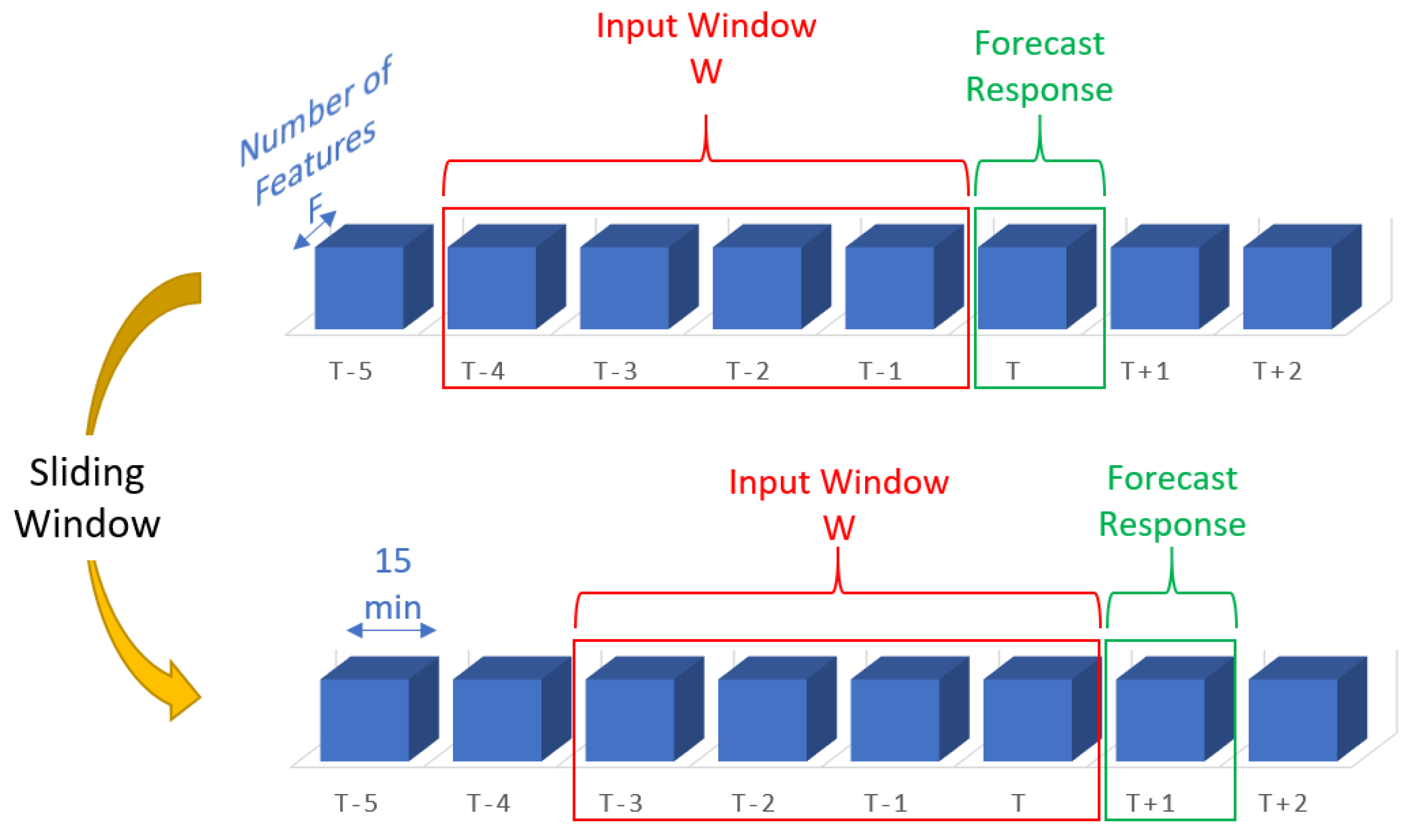
The first training sample for the input variable “” is built as a matrix with the dimensions , where is the window length (), and is the number of features. As shown in Figure 1, the window then slides forward by one step (15 min), the data from time step i + 1 create the second sample, and so on. The size of this sliding window controls how much historical data influences the prediction (e.g., 30 min, 60 min, 120 min, etc.).
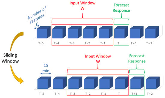
Figure 1.
Sliding Window Sampling Procedure.
A reading from a single time step can be included in numerous sliding windows and overlaps when considering the 15 min step. The final training dataset has the shape of a matrix ; is the number of rows of data in total, n is the window size (length of window) and is the number of features. The model predicts the room temperatures for T + i (output) for each sample (window length ), where i is the horizon response in the future. Each model is created to accurately predict the room temperatures at one or more alternative forecast responses, such as T + 1, T + 2, T + 3, or T + 4 (15, 30, 45, or 60 min in the future).
3.4. Performance Evaluation
To assess the model performance, three metrics were used for each test sample: mean squared error (MSE), root mean squared error (RMSE), and mean absolute error (MAE). The final score was calculated by averaging the metric scores across all samples.
where is the total number of observations, and are the actual and predicted values, respectively. MSE, MAE, and RMSE are frequently employed with time series forecasts [33,40,41]. Since the prediction error is expressed in the same units as the predicted variables, they offer a simple method for determining the prediction error. While MSE is calculated as the average of the squared differences between the predicted and actual values, RMSE gives relatively significant weight to the large errors since they are squared before being averaged and MAE evaluates the average magnitude of the errors in the prediction set. A higher accuracy of the model under consideration is implied by lower MSE, RMSE, and MAE values.
4. Machine Learning and Deep Learning Algorithms
Machine learning (ML) and deep learning (DL) are two subfields of artificial intelligence (AI) that involve the development of algorithms capable of learning from data and making predictions or decisions. While both ML and DL algorithms aim to extract patterns and insights from data, they differ in their approach and level of complexity.
Deep learning focuses on developing algorithms inspired by the structure and function of the human brain’s neural networks. DL algorithms are designed to automatically learn hierarchical representations of data by using multiple layers of interconnected artificial neurons. Machine learning algorithms often provide more interpretability, while deep learning algorithms, with their complex architectures and a large number of parameters, can be considered as “black boxes” with less interpretability. In addition, deep learning algorithms, due to their complex architectures, often require significant computational resources, while machine learning algorithms are generally less computationally demanding. In this study, we focused on deep learning algorithms as they are expected to be more suitable for the application. However, we did explore the potential of the less complex tree-based machine learning algorithms.
Five data mining algorithms, namely Extra Trees and Random Forest (RF) as tree-based algorithms and the Multilayer Perceptron (MLP), Long-Short Term Memory (LSTM), and convolutional neural networks (CNN) as deep learning algorithms have been applied to the studied HVAC system based on their proven potential in related studies. The Extra Trees and Random Forest are supervised tree-based machine learning models that solve classification or regression problems by building a tree-like structure to generate predictions. Recursively dividing the observations under consideration according to some criteria results in the construction of tree-based models. However, the MLP neural network as a deep learning algorithm is a widely used feed-forward neural network with several neurons and multiple layers. The MLP can recognize and learn patterns based on input datasets and the corresponding target values by adaptively modifying the weights in supervised learning. The LSTM is a type of neural network architecture that was designed with memory cells and gates to selectively remember or forget information in time series. On the other hand, the key innovation of CNNs lies in their use of convolutional layers that can effectively extract spatial features from raw data.
By selecting these five algorithms, a comprehensive and multi-faceted approach to indoor temperature prediction was examined. Each algorithm contributes unique capabilities that address different aspects of the problem, such as ensemble learning (Extra Trees and Random Forest algorithms) for improved accuracy, MLP for non-linear relationship modeling, LSTM for handling temporal dependencies and CNN for capturing spatial patterns. These algorithms are amongst the most popular algorithms in artificial intelligence and HVAC system modeling.
4.1. Tree-Based Algorithms
Multiple decision tree predictors are combined in ensemble methods (such as bagging and boosting) which are known as tree-based algorithms to improve performance and create more robust prediction models. The bagging method makes use of average forecasts from various trees that were built using various data subsets; meanwhile, boosting is an iterative method that fits a series of trees made from random samples. Simple models are fitted to the data at each phase, and the data are assessed for errors. In the past, several researchers have examined the efficiency of ensemble-based models for forecasting time series datasets and HVAC systems in particular [20,21,42].
4.1.1. Extra Trees
According to Alawadi et al. [20], the Extra Trees algorithm is the most precise and effective model for HVAC system temperature prediction. Therefore, the Extra Trees algorithm with randomly selected decision rules is one of the selected algorithms in this study for modeling purposes.
The sampling for each tree in the Extra Trees algorithm is random and without replacement. By sampling the complete dataset, Extra Trees avoids the biases that different subsets of the data may impose on the results. Additionally, each tree receives a specific number of features, chosen at random from the entire set of features. The random selection of a splitting value for a feature is also the most significant and distinctive aspect of Extra Trees. As a result, the trees become more diverse and uncorrelated, which reduces variance and lessens the influence of specific features or patterns in the data.
4.1.2. Random Forest
The performance of a single decision tree in regression models is unstable because the final regions are influenced by the data’s properties, and even little changes in the data might produce drastically different outcomes. Therefore, Breiman [43] suggested using random forest algorithms to produce more stable models with improved prediction accuracy. The Random Forest algorithm also showed reliable performance in dealing with time series datasets [44]. In addition, it has been frequently employed in HVAC systems for modeling purposes [26,45,46].
The Random Forest (RF) method subsamples the input data with replacement. The RF technique is based on the idea that numerous uncorrelated models work significantly better together than they do separately. With random sampling from robust decision trees, the RF algorithm decreases the risk of overfitting, while decision trees generally tend to tightly fit all the samples throughout training, which exposes them to overfitting.
4.2. Deep Learning Algorithms
A group of machine learning algorithms known as “deep learning” go beyond simple learning and focus on learning from experience [23]. These algorithms undergo many linear or non-linear transformations of the input data before obtaining an output.
Deep learning (DL) is made up of several hidden layers of neural networks that perform complex operations on massive amounts of data. Due to the superior predictive modeling applications of DL, it has advanced predictive modeling by enabling more accurate predictions and the ability to handle vast amounts of complex data, thus opening up new possibilities for data-driven insights and decision-making in a number of sectors.
DL techniques have become more popular among researchers in recent years as an alternative to manual feature extraction. This strategy has gained popularity with ANN architectures and has produced groundbreaking solutions for time series problems [47].
In this study, three deep learning algorithms are investigated: the multilayer perceptron (MLP), long short-term memory (LSTM), and convolutional neural networks (CNN). These algorithms were chosen because they are pertinent to both the application under consideration and the studied case study.
4.2.1. Multilayer Perceptron
Multilayer perceptron (MLP) is a deep learning algorithm that is one of the selected algorithms in this study because it has already demonstrated a good performance in time series prediction problems [48]. In addition, it proved its potential in HVAC systems as time-dependent systems [46,49,50]. Figure 2 shows the structure of the deep neural network model.
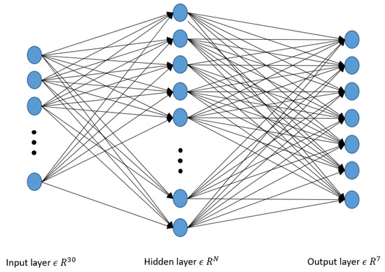
Figure 2.
Structure of the deep neural network.
By updating the weights of the neurons, the MLP algorithm has a significant capability for mapping the link between input parameters and output parameters. Three layers made up the MLP model in this study: the input layer, the hidden layer, and the output layer. First, the forward propagation process from the input layer to the output layer is created when the input parameters are added to the MLP model. Then, using a backpropagation method, the weights and thresholds between the input layer and hidden layer as well as between the hidden layer and output layer are tuned. The first and second stages are repeated until the training error can meet the desired settings.
The perceptron/neuron is the most basic learnable artificial neural network with input visible units , trainable connection weights , a bias, and an output unit as shown in Equation (4). The perceptron model is also known as a single-layer neural network since it only contains one layer of output units, excluding the visible input layer. Given an input , the value of the output unit is derived from an activation function by taking the weighted total of the inputs as follows:
where stands for a parameter set, is a connection weight vector, and is a bias. In this study, a “relu” function is utilized as the activation function and the activation variable is defined by the weighted sum of the inputs, i.e., .
As the studied HVAC system involves multiple zones, it needs to be extended to a multi-output model, so multiple output parameter vector is added to each output. The outputs’ respective connection weights are as follows:
where denotes a connection weight from to .
During the training phase, neural networks learn by iteratively adjusting the parameters (weights and biases). The biases are initially set to zero and the weights are created at random to establish the parameters. The data are then forwarded across the network to provide model output. The process of back-propagation is the last one. Several iterations of a forward pass, back propagation, and parameter update are commonly included in the model training process until the model reaches the predefined setting values, and the best parameters of the network are obtained, which could link the inputs to the outputs with a high accuracy or low error, even in highly non-linear and sophisticated systems.
4.2.2. Long Short-Term Memory (LSTM)
LSTM topology has been presented as a way to directly integrate time dependence. The fundamental concept is to dynamically integrate a sequential structure in order to enhance the functionality of conventional ANN approaches [51]. LSTM has demonstrated exceptional performance because it can learn the short- and long-term dependencies. The simultaneous inclusion of slow- and fast-moving phenomena makes LSTM a good option for indoor temperature prediction problems [52]. Time series data processing and prediction are all very well suited to LSTM networks [34,53]. The LSTM algorithm was considered in this research since it can capture features and remember them over time. A typical illustration of an LSTM cell is shown in Figure 3.
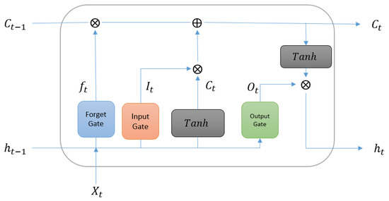
Figure 3.
A typical LSTM neuron structure.
When compared to cutting-edge black-box modeling techniques used for indoor temperature prediction, ANN-based algorithms have high predictive power. Moreover, recurrent neural network-based methods, particularly LSTM, have an outstanding capacity for “learning” the dynamics of non-linear problems with time dependency.
4.2.3. Convolutional Neural Networks (CNN)
Convolutional neural networks, generally known as CNNs, are powerful types of artificial neural networks and deep learning algorithms. CNNs have been demonstrated to be very successful in a variety of computer vision tasks such as image classification, object recognition, and segmentation. According to their design, CNNs can automatically and adaptively learn spatial feature hierarchies from basic to complex patterns. The feature extraction is carried out by the convolution and pooling layers, and then it is mapped by the fully connected layer into a final output [54].
In general, CNNs are effective tools for processing and interpreting complicated data because of their hierarchical structure and learnable filters. Due to the proven capability and success of CNNs in solving time series problems [55], CNN is also considered in this study.
5. Case Study
Numerous initiatives have been implemented on the Burnaby campus of the British Columbia Institute of Technology to reduce environmental impacts of its educational buildings. One of these initiatives aims to reduce BCIT’s greenhouse gas emissions by 33% by 2023 [56]. Therefore, the primary objective of this study is to develop a model to predict indoor temperatures which can provide a meaningful way to reduce the energy consumption of the system and meet the requirement of greenhouse gas emissions reduction at BCIT.
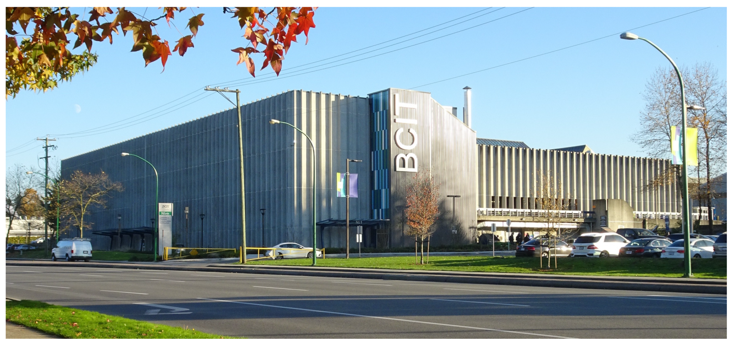
The British Columbia Institute of Technology (BCIT) is located in the city of Burnaby, BC, Canada. It is a post-secondary institution with 62 buildings and five campuses. The HVAC system under study is owned and operated by BCIT at the Burnaby Campus. The investigated HVAC system is installed at the NE01 building (NE stands for North East). The building is 20,076.88 of gross floor area consisting of offices, classrooms, restrooms, and mechanical rooms. NE01 is a 4-floor educational building dedicated to the Construction and Environmental Department at the Burnaby campus; see Figure 4.

Figure 4.
NE01 building overview.
The selection of the NE01 building for this research was based on several key factors, namely its high energy consumption compared to other buildings in the BCIT campus, the alignment with BCIT’s sustainability goals, the availability of archived data over many years for multiple zones served by the same system, and the potential for implementation of the proposed solution to prove significant energy savings and improved occupant experience.
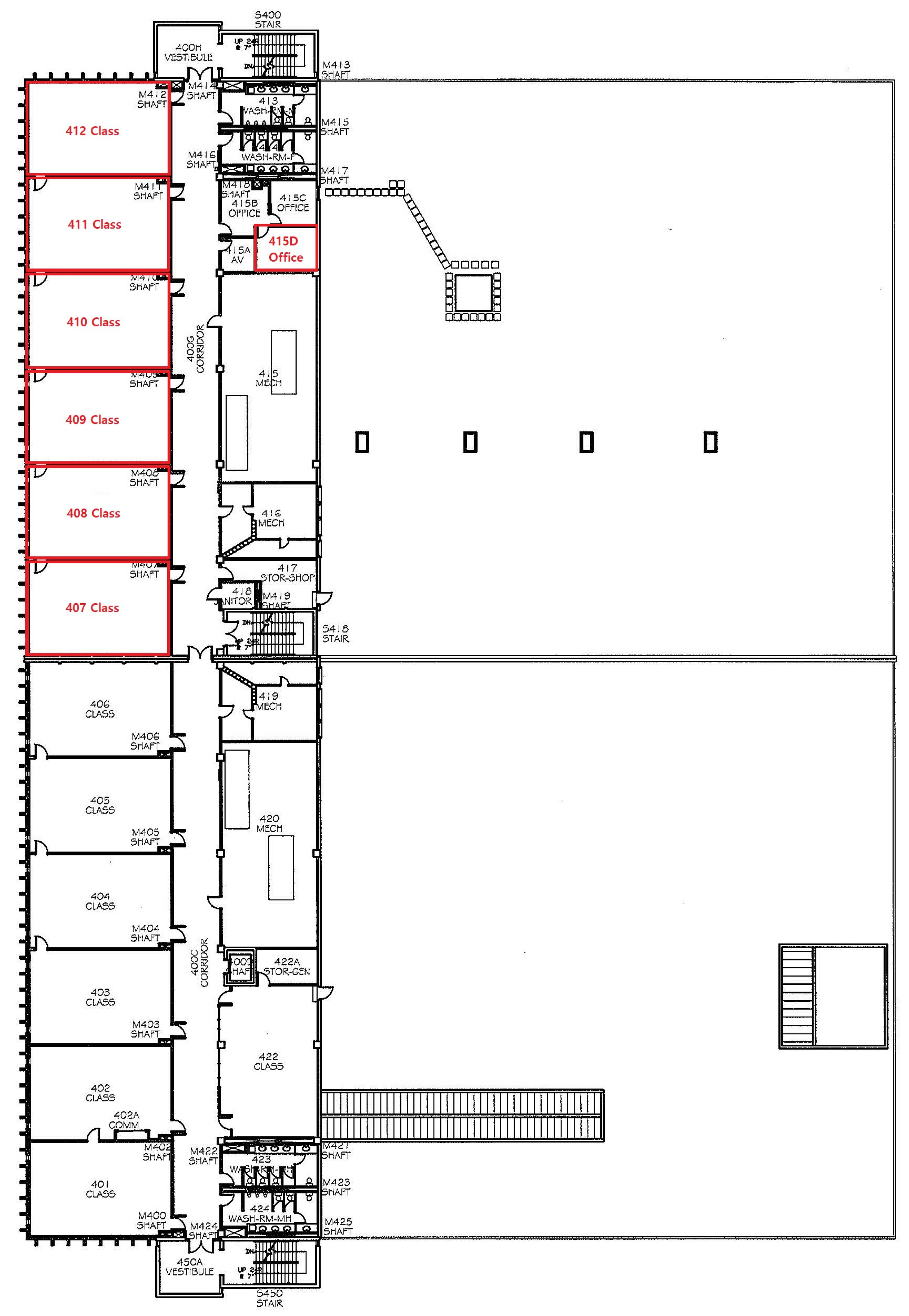
The temperatures in the NE01 building zones are controlled by ten independent Air Handling Units (AHUs). In this study, the data and parameters of one AHU (AHU7) are investigated. AHU7 delivers air to seven Variable Air Volume (VAV) units, serving seven interior zones on the fourth floor (top floor) of building NE01. The zones consist of six classrooms and an office area as shown on the floor plan of Figure 5. The BMS is used to collect the data from sensors and virtual meters of the air handling system.

Figure 5.
Schematic of the zones supplied by AHU7.
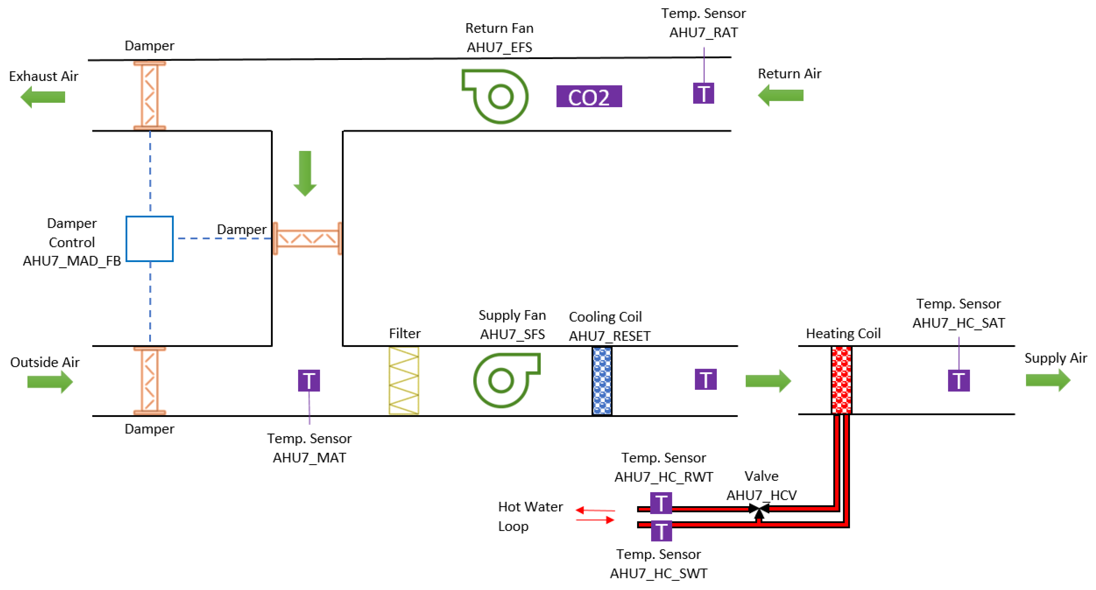
Figure 6 shows a schematic diagram of AHU7 with the available monitored parameters. Airflow is controlled via the supply and return fans. Recirculated air from the seven service zones is mixed with outdoor air and reconditioned through the AHU. The mixed-air conditions are controlled by three dampers regulating the percentages of air exhausted from the system, entering the system, and recirculating in the system. The mixed air is pulled through the filter via the supply fan and then cooled or heated when passing through the cooling and heating coils. The heating coil uses hot water supplied by the boiler. Heating is controlled by adjusting the flow of water through the coil, which is controlled by an electronic valve.
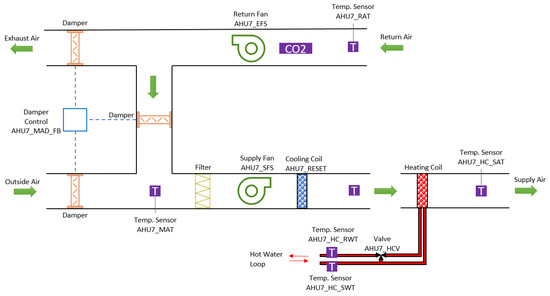
Figure 6.
Schematic diagram of AHU7.
AHU7 serves seven VAV units to further condition the supplied air to meet the required temperature by each zone. The seven reheat systems have the same design. Figure 7 represents a sample VAV box and the reheat system for each zone. Air is supplied by the AHU to the VAV boxes, which control the amount of air that is supplied to the zone by a VAV damper. At the VAV, the air also passes through a reheat coil to be warmed based on the temperature required in the zone. Similar to the heating coil at the AHU level, the reheating coil uses hot water supplied by the boiler, and it is controlled by an electronic valve to adjust the flow of water in the coil.

Figure 7.
VAV box and reheat coil subsystem for each zone.
6. Description of Available Data
The facilities department at BCIT has adopted an advanced BMS over the past few years. The data from many of the system sensors has been recorded and archived since 2016. Due to the COVID-19 pandemic, there was very little activity on campus between March 2020 and September 2021. Therefore, the data from this period were not considered for this application of predictive modeling. The data used for this study are for two periods. The first period is from February 2016 to December 2019, and the second period is from September 2021 to November 2022.
The first period represents almost four years and about 140,000 data points per system component, and the second period represents 14 months and about 40,000 data points; in total, about 180,000 data points were considered. Each row of these data corresponds directly to the state of the system at 15 min time intervals. Among the studied dataset, last year’s data were assigned as the test dataset, and the remaining data were divided into two parts: 80 percent was used for training models, and 20 percent for validation purposes.
7. Parameter Selection
Since it is too complicated to establish the mapping between inputs and outputs using all features, parameter selection is a crucial step before building a data-driven model. A typical HVAC system is a complex, non-linear network with hundreds of parameters reflecting every particular element. While some of the data obtained are closely related to the result, others are unnecessary or redundant for the modeling process. In data mining, the inclusion of redundant or unnecessary parameters may hide primary trends. Additionally, redundant parameters substantially or entirely replicate the data in one or more other parameters, making the model considerably more challenging than it has to be. The accuracy, scalability, and understandability of the resulting models may be enhanced by removing irrelevant or related characteristics. In addition, by reducing the dimensionality, a model’s complexity may also be significantly reduced [57].
For a preliminary analysis, a dataset with 75 parameters was selected based on the domain knowledge. To determine how closely parameters were coupled, a correlation analysis was applied. The range of the correlation between two parameters is from −1 to 1. The two features are positively associated if the correlation coefficient is greater than 0, and the higher the number, the stronger the correlation. For example, in this study, the correlation analyzes illustrated that Return Fan Speed and Supply Fan Speed were highly correlated with correlation equal to 1. It means Supply and Return Fan Speeds were changing at the same rate, and both were also correlated with the Status of the Return Fan with a 0.98 correlation. These are expected because the blowing air into the zones must be exhausted, and if the building is made tight enough, return fans are good controllable options to control the exhausted air. Similarly, other highly correlated parameters were diagnosed and eliminated from the list of input parameters in order to reduce the model complexity and also to reduce the risk of overfitting. With this method, the number of parameters was reduced from 75 to 57 parameters.
To increase the computational efficiency and lower the generalization error, a sequential backward feature selection approach was used to reduce the dimensionality of the initial feature subspace from N- to K-features with a minimum reduction in model performance [58]. Sequential backward feature selection was initialized by considering a feature set containing available predictors in the dataset. The regression model was trained using these features and its performance was evaluated using mean squared error (MSE). Iteratively, one feature at a time was removed from the current feature set. After each removal, the regression model was retrained, and its performance was assessed using the chosen evaluation metric. Then, the performance of the regression model with the reduced feature subset was compared to the performance achieved with the previous feature set. If the performance dropped beyond a predefined threshold or significantly deteriorated, the process was stopped, and the previous feature set was retained as the final selection. However, if the performance did not decrease significantly, the next iteration proceeded. The removal and evaluation steps were repeated until the stopping criterion was satisfied. Features with the highest impact on error rate indicated a larger contribution to the predicted output parameters. Based on the domain knowledge, correlation consideration of parameters and the sequential backward feature selection results, the final set of variables reached 24 features.
In addition, as the studied zones are on the top floor of the building and through the roof they are exposed to solar radiation, the solar radiation and outdoor air temperature data were also added to the dataset. The data were recorded by the sensors installed on the nearby weather station on the campus, and because of their stochastic nature, solar radiation and outdoor air temperature were considered as external disturbances. The selected 26 parameters are shown in Table 1.

Table 1.
Parameters Description.
Furthermore, the HVAC system under consideration operates on set schedules. Based on the operational specifications, schedules change depending on the day of the week (weekday/weekend), the hour of the day, as well as holidays. The RTs were affected by this operation schedule. Therefore, the characteristics that reflect seasonality such as the hour of the day and the day of the week (weekday/weekend) were also used as inputs in an effort to capture the temporal dependency in the model. The schedule-based variables that were specified as input features for the prediction models are listed in Table 2. Therefore, the total number of input parameters was 30.

Table 2.
Schedule-based features.
8. Results and Discussion
The five algorithms detailed in Section 4 were trained to predict indoor temperatures up to a 60 min forecast horizon with 15 min intervals and 30 min, 60 min, and 120 min sliding window sizes. Since the forecast horizon (T + 1, T + 2, etc.) and the time delay of input variables (sliding window width) have a major impact on the prediction model accuracy, various combinations of the two parameters are established in order to examine their interaction. The width of sliding windows of 2 (30 min), 4 (60 min), and 8 (120 min) time steps was investigated. As the system is notably changing fast, a lookback window beyond 120 min appears unnecessary and could potentially introduce noise to the prediction results without conferring any benefits. In addition, the RTs for the 15 to 60 min forecast horizon were predicted using the model since the equipment shows a rapid response to control commands.
First of all, the model architecture was trained to predict indoor thermal temperatures in each zone supplied by VAVs, while the evaluation metrics were calculated for different window lengths and prediction horizons.
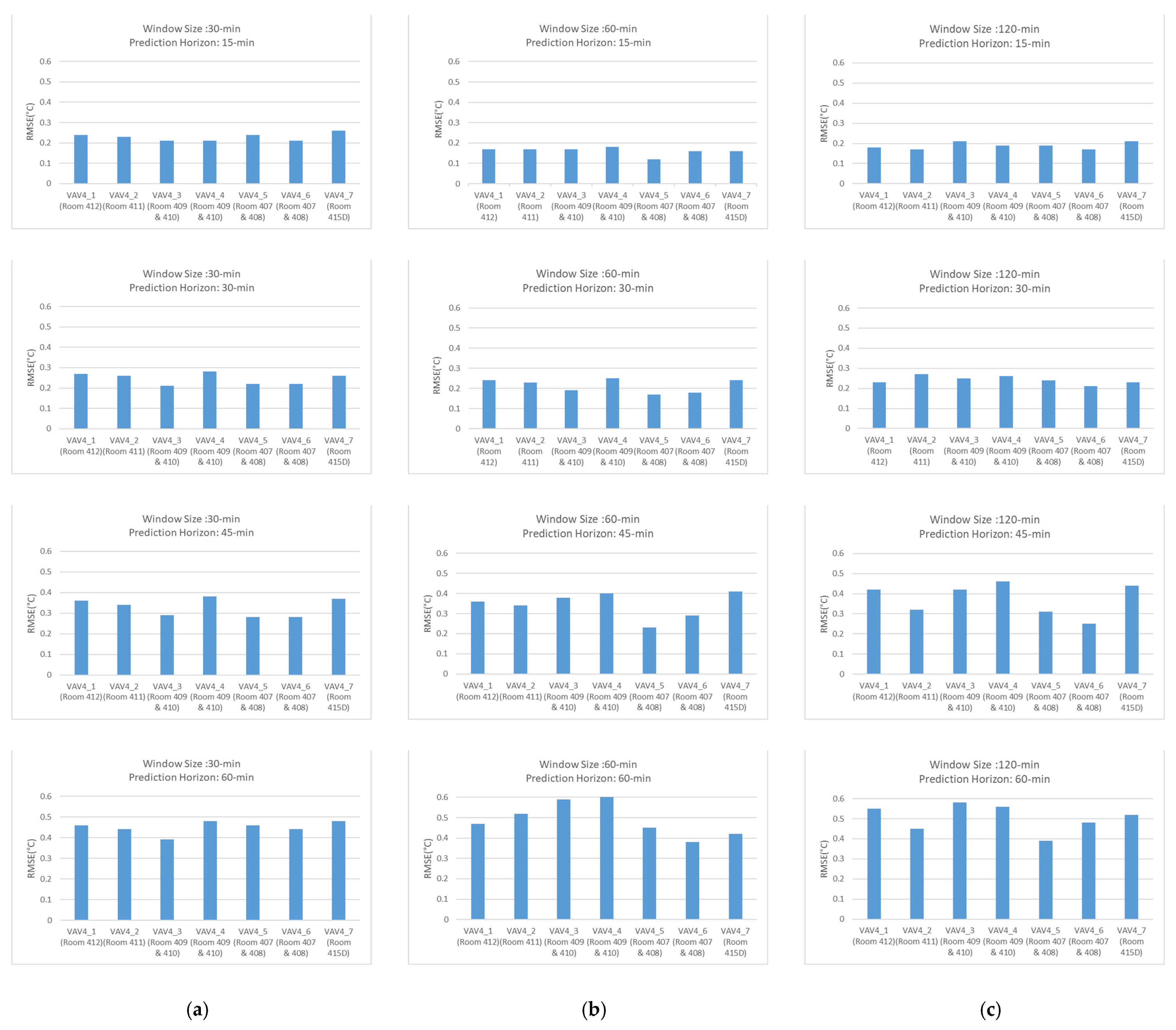
Figure 8 illustrates the RMSE obtained on the test dataset for various lookback sliding windows on the MLP model. The metrics for the error analysis evaluation are plotted against the window length and forecast horizon to show that the model performance degrades when the forecast horizon increases and the window length goes beyond 30 min. For a prediction of 15 min ahead, the lowest errors were observed for a sliding window of 60 min. The size of the lookback window has an insignificant effect on the prediction when it is one hour or beyond.
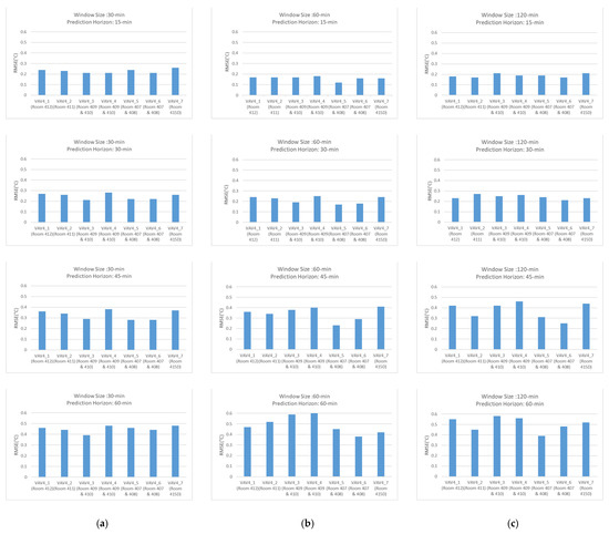
Figure 8.
Error analysis evaluation on window length and forecast horizon of the proposed MLP model. (a) 30 min lookback window; (b) 60 min lookback window; (c) 120 min lookback window.
The investigation of the sliding window and forecast horizon effect on the RMSE was applied to all studied algorithms, and for all of them, similar results were seen. Thus, the best window length for the sliding window sampling method was selected as 60 min with 15 min forecast horizon as it resulted in the lowest RMSE in the seven zones; therefore, it was applied for training the final developed model.
The MSE, RMSE, and MAE for the two tree-based machine learning algorithms and the deep learning models are shown in Table 3 and Table 4 for the 15 min forecast horizon. The performance of the different architectures was assessed. It was noted that all models exhibit comparable overall prediction accuracy. Although the ML and DL models under consideration can predict the RTs with an acceptable error, the rate of their errors was analyzed in detail. The model sensitivity is crucial since this analysis is a critical part of a larger study that aims to represent a digital twin of the studied HVAC system for long-term predictions and application of energy optimization strategies.

Table 3.
The 15 min prediction horizon error [C] of validation and test datasets of the trained tree-based algorithm models for the seven zones supplied by AHU7.

Table 4.
The 15 min prediction horizon error [C] of validation and test datasets of the trained deep learning algorithm models for the seven zones supplied by AHU7.
According to Table 3 and Table 4, the Extra Trees and Random Forest algorithms are the least accurate compared to the deep learning algorithms. This demonstrates the necessity of more complex ML and DL algorithms that learn time dependency and patterns of room temperature changes over time. It was noticed that the average RMSE rate on the test dataset for all seven room temperatures was 0.36 °C for Random Forest and 0.35 °C for Extra Trees algorithms. All the deep learning algorithms outperformed tree-based algorithms and showed a lower RMSE rate on test datasets with an average RMSE of 0.16 °C. In addition, the difference between the MSE results of the deep learning algorithms in validation and test datasets with an average of 0.01 is insignificant, which means a low variance in the proposed models. In contrast, the MSE error difference between validation and test datasets for tree-based algorithms is higher. It shows the higher capability of the deep learning algorithms in modeling indoor temperatures compared to the Extra Trees and the Random Forest algorithms.
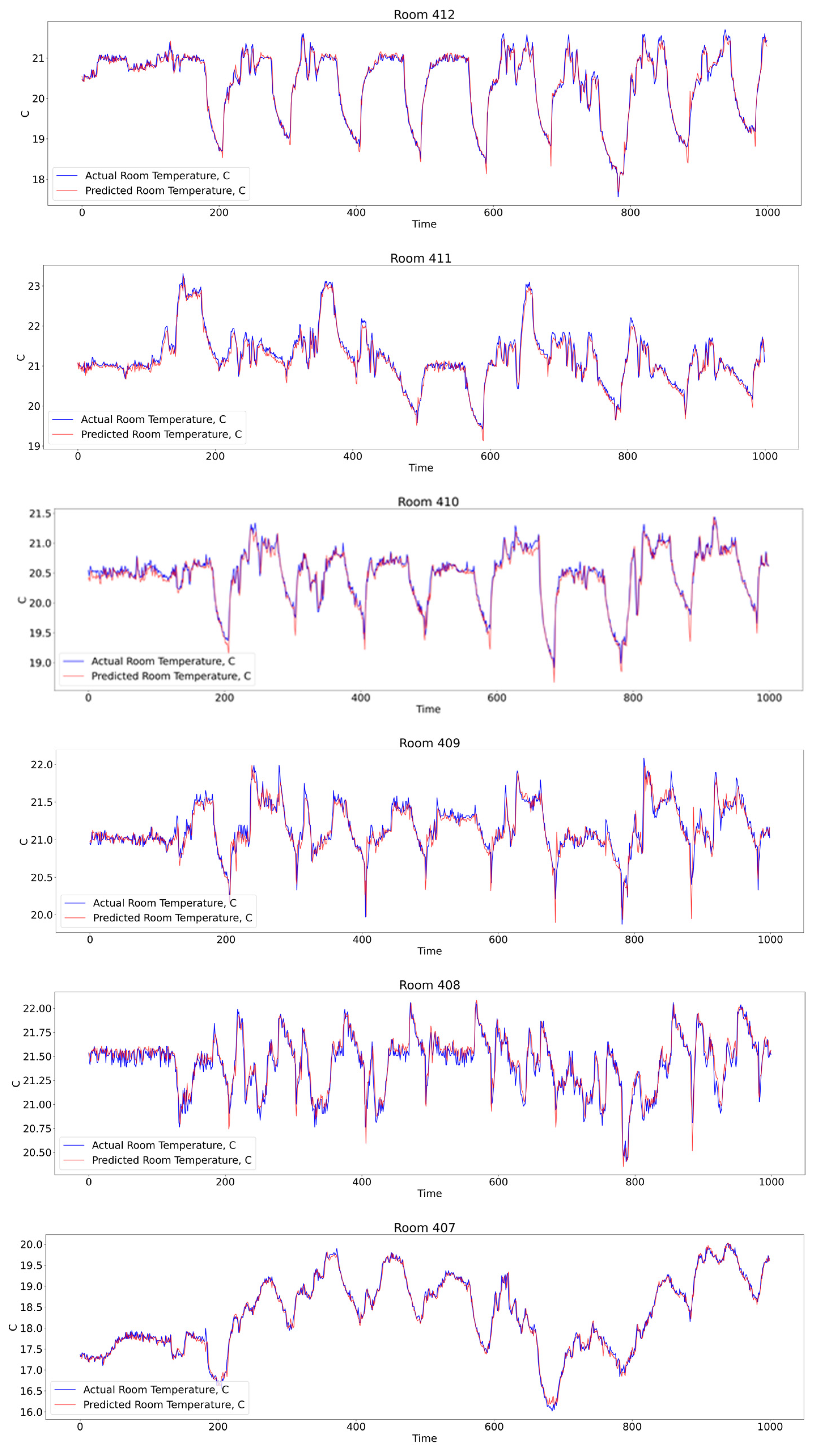
Additionally, it was noted that the RMSE values of both the validation and test sets for each of the investigated algorithms are higher than the MSE and MAE. This is a reference to the samples in the dataset having significant error levels. A detailed examination of the significant errors revealed that the models perform poorly in forecasting abrupt changes in room temperatures. Therefore, the larger error instances were checked and analyzed and it was noticed that at harsh temperature changes, the prediction error sometimes can surpass ±0.8 °C. However, the number of samples with this error rate is below 0.2% on the whole samples in the dataset. Samples with high errors can be treated as outliers in the modeling process, hence they are considered as a nature of the current system in this study which is part of the existing HVAC systems. In addition, investigations showed that high prediction errors are recorded in the early mornings and at the end of the day when the HVAC system starts and stops based on schedules. During these transitions, considerably different set points are assigned to the system abruptly, which leads to harsh temperature changes in a short time period. Appendix A illustrates a snapshot of the predicted room temperatures versus actual room temperatures in each zone.
It should be noted that direct comparison of the results presented in this paper with those of other published studies is not feasible due to variations in factors such as the buildings considered, input parameter sets employed, and quantities of collected data utilized. However, the modeling quality achieved in terms of RMSE, MSE, and MAE in this study is comparable to the outcomes reported in other published researches. Table 5 lists a concise summary of the deep learning model results from previous studies. The predictions of room temperatures obtained in this study through the utilization of deep learning algorithms show superior performance when compared to the outcomes of previous comparable relevant studies.

Table 5.
Performance of ANN models for indoor temperature predictions in previous works.
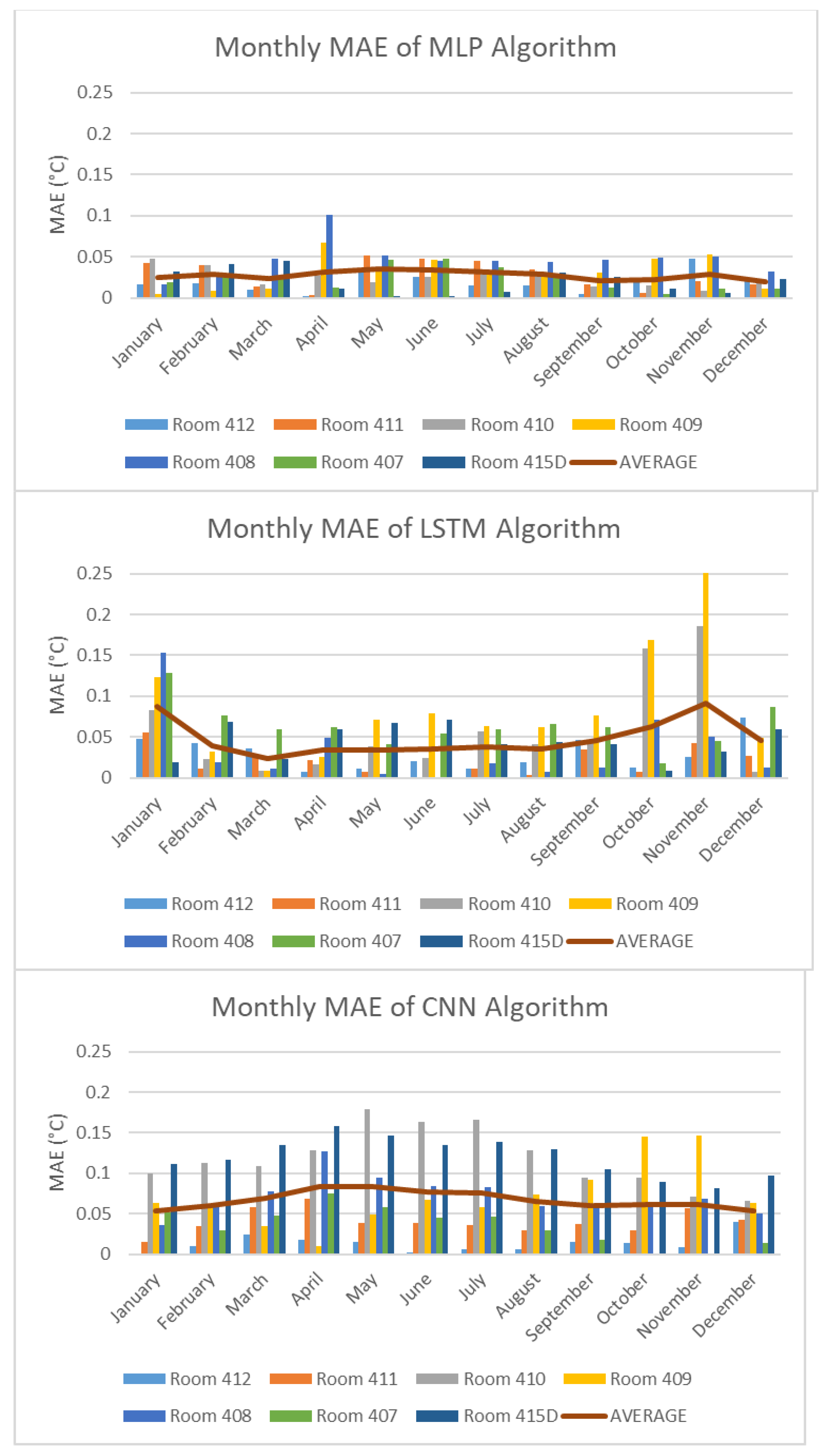
Figure 9 shows the distribution of the average MAE per month across the year in detail for the studied zones. It was found that all deep learning models can predict all room temperatures with high accuracy all over the year. The high errors are captured in the prediction of the transition period (April to June) during spring and then these decrease during the summer months and again they start to gradually increase from September to November almost in all algorithms. It means that the models are less accurate in predicting indoor temperatures during these periods, for example, in the spring when heating is on and cooling starts to take over the control of the HVAC system.
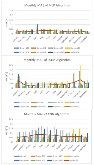
Figure 9.
Distribution of monthly mean absolute errors.
In addition, Figure 9 shows the MAE of the MLP algorithm for all seven zones is more consistent compared to the other algorithms. The LSTM and CNN algorithms predict each individual zones at monthly highly different error rates, while the MLP algorithm is producing more persistent results for all zones. In other words, LSTM and CNN algorithms can predict some of the zones with high accuracy, while prediction errors of some other zones can be twice (or more) as prevalent.
The purpose of this study was first to determine how well algorithms predict HVAC parameters and then to select the best model settings for predicting room temperatures in each zone. Based on the performance evaluation detailed above, it was found that the deep learning models outperform the tree-based models. Specifically, the MLP model showed a more consistent and accurate prediction among the investigated deep learning models. This is a promising result leading to the potential employment of the MLP model and more generally the LSTM and CNN models to adjust the equipment setting of the HVAC in real-time, without human involvement and scheduled rules.
9. Conclusions
Accurate indoor temperature prediction is necessary to develop HVAC system digital twin that can eventually provide opportunities to optimize building energy consumption and maintain indoor thermal comfort. The main goal of this study was to suggest the most accurate data-driven model for HVAC systems. In this regard, this study investigated five suitable algorithms to predict indoor temperatures of a multi-zone HVAC system of an educational building. Seven room temperatures supplied by an AHU and seven VAVs at the NE01 building of the British Columbia Institute of Technology were predicted using five algorithms and collected real data.
Firstly, feature selection techniques were applied to determine the most critical features. The effectiveness of the proposed feature selection methods was successfully demonstrated as they proved capable of identifying significant and independent input parameters without compromising the overall prediction performance. This highlights the robustness and reliability of the feature selection methods in determining the most relevant features while ensuring that the prediction accuracy is high.
This study investigated machine learning and deep learning algorithms and proved that the latter produced better outcomes throughout the analysis with an average RMSE of 0.16 °C. The MLP algorithm as a deep learning model produced the best results compared to the other investigated deep learning algorithms with its consistent and stable prediction throughout the months of the year. It was demonstrated that room temperatures could be precisely predicted within a 15 min forecast horizon in advance using the developed MLP deep learning algorithm. As a result, the study offers the most accurate algorithm for development of a digital twin that includes various HVAC systems and the rooms they service in a specific educational building. Regarding building a digital twin model, the proposed model will be utilized and addressed in future work to simulate and produce the best settings for the studied HVAC system, which would result in lower energy consumption without sacrificing the occupant’s comfort level.
In this study, the test dataset spans a whole year. Therefore, a more thorough analysis of the models’ performance during this time is necessary. Using whole-year data could lead to less accurate transitional period predictions because no input variables have been provided to address transitions over the months in this study. In addition, occupancy level parameters are not included as a predictor variable, so their effect is not considered during the modeling process. A qualitative consideration revealed that some significant errors are the result of unexpected indoor activities, such as high occupancy levels during particular periods. Future research could further increase prediction accuracy by incorporating the scheduled occupancy data and analysis of the influence of heat and humidity produced by occupants, where the “full” effect of occupants can be considered.
Author Contributions
Conceptualization, S.M.; Formal analysis, P.N.; Investigation, P.N.; Resources, R.M.; Data curation, P.N.; Writing—original draft, P.N.; Supervision, S.M. and R.M.; Project administration, R.M.; Funding acquisition, S.M. All authors have read and agreed to the published version of the manuscript.
Funding
This work was supported by the Institute Research Fund granted by the British Columbia Institute of Technology.
Data Availability Statement
Data sharing not applicable. No new data were created or analyzed in this study. Data sharing is not applicable to this article.
Acknowledgments
The authors would like to express their sincere gratitude to the British Columbia Institute of Technology for supporting this project. The facilities department and the Energy Team are also acknowledged for their invaluable support, guidance, and assistance throughout the processes of case study selection and data collection.
Conflicts of Interest
The authors declare no conflict of interest.
Appendix A
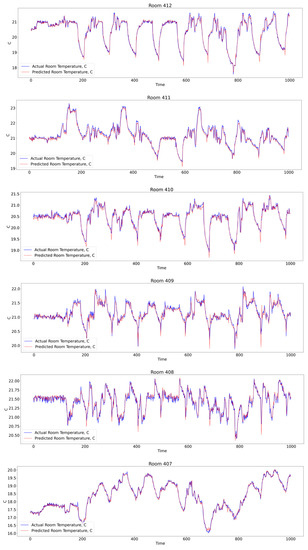

Figure A1.
The 15 min ahead and 1 h sliding window predicted indoor temperature for the MLP model.
Figure A1.
The 15 min ahead and 1 h sliding window predicted indoor temperature for the MLP model.

References
- International Energy Agency. International Energy Outlook 2006, June 2006. Available online: https://www.iea.org/reports/world-energy-outlook-2006 (accessed on 1 June 2023).
- Perez-Lombard, L.; Ortiz, J.; Pout, C. A Review on Buildings Energy Consumption Information. Energy Build. 2008, 40, 394–398. [Google Scholar] [CrossRef]
- Natural Resources Canada. Report Energy Fact Book; Natural Resources Canada: Ottawa, ON, Canada, 2021. [Google Scholar]
- Bourdeau, M.; Zhai, X.Q.; Nefzaoui, E.; Guo, X.; Chatellier, P. Modeling and forecasting building energy consumption: A review of data-driven techniques. Sustain. Cities Soc. 2019, 48, 101533. [Google Scholar] [CrossRef]
- Braun, J.E.; Chaturvedi, N. An inverse gray-box model for transient building load prediction. HVAC R Res. 2002, 8, 73–99. [Google Scholar] [CrossRef]
- Maasoumy, M.; Razmara, M.; Shahbakhti, M.; Sangiovanni-Vincentelli, A. Handling Model Uncertainty in Model Predictive Control for Energy Efficient Buildings. Energy Build. 2014, 77, 377–392. [Google Scholar] [CrossRef]
- Hao, H.; Kowli, A.; Lin, Y.; Barroah, P.; Meyn, S. Ancillary Service for the Grid via Control of Commercial Building HVAC Systems. In Proceedings of the American Control Conference, Washington, DC, USA, 17–19 June 2013. [Google Scholar]
- Jeong, K.; Koo, C.; Hong, T. An estimation model for determining the annual energy cost budget in educational facilities using SARIMA, (seasonal autoregressive integrated moving average) and ANN (artificial neural network). Energy 2014, 71, 71–79. [Google Scholar] [CrossRef]
- Zhang, F.; Deb, C.; Lee, S.E.; Yang, J.; Shah, K.W. Time series forecasting for building energy consumption using weighted support vector regression with differential evolution optimization technique. Energy Build. 2016, 126, 94–103. [Google Scholar] [CrossRef]
- Ahmad, M.W.; Mourshed, M.; Rezgui, Y. Trees vs neurons: Comparison between random forest and ann for high-resolution prediction of building energy consumption. Energy Build. 2017, 147, 77–89. [Google Scholar] [CrossRef]
- Huang, Y.; Miles, H.; Zhang, P. A sequential modelling approach for indoor temperature prediction and heating control in smart buildings. arXiv 2020, arXiv:2009.09847. [Google Scholar]
- Ogunmolu, O.; Gu, X.; Jiang, S.; Gans, N. Nonlinear systems identification using deep dynamic neural networks. arXiv 2016, arXiv:1610.01439. [Google Scholar]
- Ferreira, P.; Ruano, A.; Silva, S.; Conceição, E. Neural networks based predictive control for thermal comfort and energy savings in public buildings. Energy Build. 2012, 55, 238–251. [Google Scholar] [CrossRef]
- Nassif, N.; Moujaes, S. A cost-effective operating strategy to reduce energy consumption in a HVAC system. Int. J. Energy Res. 2008, 32, 543–558. [Google Scholar] [CrossRef]
- Nassif, N.; Kajl, S.; Sabourin, R. Evolutionary algorithms for multi-objective optimization in HVAC system control strategy. Fuzzy Inf. 2004, 1, 51–56. [Google Scholar]
- Nassif, N.; Kajl, S.; Sabourin, R. Optimization of HVAC control system strategy using two objective genetic algorithm. HVAC R Res. 2005, 11, 459–486. [Google Scholar] [CrossRef]
- Platt, G.; Li, J.; Li, R.; Poulton, G.; James, G.; Wall, J. Adaptive HVAC zone modeling for sustainable buildings. Energy Build. 2010, 42, 412–421. [Google Scholar] [CrossRef]
- Goyal, S.; Barooah, P. A Method for Model-Reduction of Nonlinear Thermal Dynamics of Multi-Zone Buildings. Energy Build. 2012, 47, 332–340. [Google Scholar] [CrossRef]
- Wang, S.; Ma, Z. Supervisory and optimal control of building HVAC systems: A Review. HVAC R Res. 2008, 14, 3–32. [Google Scholar] [CrossRef]
- Alawadi, S.; Mera, D.; Fernández-Delgado, M.; Alkhabbas, F.; Olsson, C.M.; Davidsson, P. A comparison of machine learning algorithms for forecasting indoor temperature in smart buildings. Energy Syst. 2020, 13, 689–705. [Google Scholar] [CrossRef]
- Ampomah, E.K.; Qin, Z.; Nyame, G. Evaluation of Tree-Based Ensemble Machine Learning Models in Predicting Stock Price Direction of Movement. Information 2020, 11, 332. [Google Scholar] [CrossRef]
- Manivannan, M.; Behzad, N.; Rinaldi, F. Machine Learning-Based Short-Term Prediction of Air-Conditioning Load through Smart Meter Analytics. Energies 2017, 10, 1905. [Google Scholar] [CrossRef]
- Fan, C.; Xiao, F.; Zhao, Y. A short-term building cooling load prediction method using deep learning algorithms. Appl. Energy 2017, 195, 222–233. [Google Scholar] [CrossRef]
- Kusiak, A.; Xu, G.; Zhang, Z. Minimization of energy consumption in HVAC systems with data-driven models and an interior-point method. Energy Convers. Manag. 2014, 85, 146–153. [Google Scholar] [CrossRef]
- Ben-Nakhi, A.E.; Mahmoud, M.A. Energy conversation in buildings through efficient A/C control using neural networks. Appl. Energy 2002, 73, 5–23. [Google Scholar] [CrossRef]
- Wei, X.; Kusiak, A.; Li, M.; Tang, F.; Zeng, Y. Multi-objective optimization of the HVAC (heating, ventilation, and air conditioning) systems performance. Energy 2015, 83, 294–306. [Google Scholar] [CrossRef]
- Kusiak, A.; Tang, F.; Xu, G. Multi-objective optimization of HVAC system with an evolutionary computation algorithm. Energy 2011, 36, 2440–2449. [Google Scholar] [CrossRef]
- Thomas, B.; Soleimani-Mohseni, M. Artificial neural network models for indoor temperature prediction: Investigations in two buildings. Neural Comput. Appl. 2007, 16, 81–89. [Google Scholar] [CrossRef]
- Mirzaei, P.A.; Haghighat, F.; Nakhaie, A.A.; Yagouti, A.; Giguere, M.; Keusseyan, R.; Coman, A. Indoor thermal condition in urban heat Island—Development of a predictive tool. Build. Environ. 2012, 57, 7–17. [Google Scholar] [CrossRef]
- Attoue, N.; Shahrour, I.; Younes, R. Smart building: Use of the artificial neural network approach for indoor temperature forecasting. Energies 2018, 11, 395. [Google Scholar] [CrossRef]
- Mba, L.; Meukam, P.; Kemajou, A. Application of artificial neural network for predicting hourly indoor air temperature and relative humidity in modern building in humid region. Energy Build. 2016, 121, 32–42. [Google Scholar] [CrossRef]
- Afroz, Z.; Urmee, T.; Shafiullah, G.M.; Higgins, G. Real-time prediction model for indoor temperature in a commercial building. Appl. Energy 2018, 231, 29–53. [Google Scholar] [CrossRef]
- Lu, T.; Viljanen, M. Prediction of indoor temperature and relative humidity using neural network models: Model comparison. Neural Comput. Appl. 2009, 18, 345–357. [Google Scholar] [CrossRef]
- Xu, C.; Chen, H.; Wang, J.; Guo, Y.; Yuan, Y. Improving prediction performance for indoor temperature in public buildings based on a novel deep learning method. Build. Environ. 2019, 148, 128–135. [Google Scholar] [CrossRef]
- Jiang, B.; Gong, H.; Qin, H.; Zhu, M. Attention-LSTM architecture combined with Bayesian hyperparameter optimization for indoor temperature prediction. Build. Environ. 2022, 224, 109536. [Google Scholar] [CrossRef]
- Makridakis, S.; Spiliotis, E.; Assimakopoulos, V. Statistical and machine learning forecasting methods: Concerns and ways forward. PLoS ONE 2018, 13, e0194889. [Google Scholar] [CrossRef]
- Weron, R. Electricity price forecasting: A review of the state-of-the-art with a look into the future. Int. J. Forecast. 2014, 30, 1030–1081. [Google Scholar] [CrossRef]
- Ozbalta, T.G.; Sezer, A.; Yildiz, Y. Models for prediction of daily mean indoor temperature and relative humidity: Education building in Izmir, Turkey. Indoor Built Environ. 2012, 21, 772–781. [Google Scholar] [CrossRef]
- Khalid, S.; Khalil, T.; Nasreen, S. A survey of feature selection and feature extraction techniques in machine learning. In Proceedings of the Science and Information Conference, London, UK, 27–29 August 2014; IEEE: Piscataway, NJ, USA, 2014; pp. 372–378. [Google Scholar]
- Galicia, A.; Talavera-Llames, R.; Troncoso, A.; Koprinska, I.; Martínez-Álvarez, F. Multi-step forecasting for big data time series based on ensemble learning. Knowl.-Based Syst. 2019, 163, 830–841. [Google Scholar] [CrossRef]
- Fan, C.; Sun, Y.; Zhao, Y.; Song, M.; Wang, J. Deep learning-based feature engineering methods for improved building energy prediction. Appl. Energy 2019, 240, 35–45. [Google Scholar] [CrossRef]
- Maalej, S.; Lafhaj, Z.; Yim, J.; Yim, P.; Noort, C. Prediction of HVAC System Parameters Using Deep Learning. In Proceedings of the 12th Conference of IBPSA, Ottawa, ON, Canada, 22–23 June 2022. [Google Scholar]
- Breiman, L. Random forests. MLear 2001, 45, 5–32. [Google Scholar]
- Qiu, X.; Zhang, L.; Suganthan, N.; Amaratunga, G.A.J. Oblique random forest ensemble via Least Square Estimation for time series forecasting. Inf. Sci. 2017, 420, 249–262. [Google Scholar] [CrossRef]
- Tang, F.; Kusiak, A.; Wei, X. Modeling and short-term prediction of HVAC system with a clustering algorithm. Energy Build. 2014, 82, 310–321. [Google Scholar] [CrossRef]
- Kusiak, A.; Li, M. Reheat optimization of the variable-air-volume box. Energy 2010, 35, 1997–2005. [Google Scholar] [CrossRef]
- Li, D.; Zhang, J.; Zhang, Q.; Wei, X. Classification of ECG signals based on 1D convolution neural network. In Proceedings of the 19th IEEE International Conference on E-Health Networking, Applications and Services, Dalian, China, 12–15 October 2017; pp. 1–6. [Google Scholar]
- Wong, F.S. Time series forcasting using backpropagation neural networks. Neurocumputing 1990, 91, 147–159. [Google Scholar]
- Kusiak, A.; Li, M. Cooling output optimization of an air handling unit. Appl. Energy 2010, 87, 901–909. [Google Scholar] [CrossRef]
- Kusiak, A.; Li, M.; Tang, F. Modeling and optimization of HVAC energy consumption. Appl. Energy 2010, 87, 3092–3102. [Google Scholar] [CrossRef]
- Mandic, D.; Chambers, J. Recurrent Neural Networks for Prediction: Learning Algorithms. In Architectures and Stability; Wiley: Chichester, UK, 2001. [Google Scholar]
- Afram, A.; Janabi-Sharifi, F. Theory and applications of HVAC control systems—A review of model predictive control (MPC). Build. Environ. 2014, 72, 343–355. [Google Scholar] [CrossRef]
- Sülo, I.; Keskin, S.R.; Dogan, G.; Brown, T. Energy efficient smart buildings: LSTM neural networks for time series prediction. In Proceedings of the 2019 International Conference on Deep Learning and Machine Learning in Emerging Applications (Deep-ML), Istanbul, Turkey, 26–28 August 2019; IEEE: Piscataway, NJ, USA, 2019. [Google Scholar]
- Yamashita, R.; Nishio, M.; Gian Do Kinh, R.; Togashi, K. Convolutional Neural Networks: An Overview and Application in Radiology. Insights Imaging 2018, 9, 611–629. [Google Scholar] [CrossRef] [PubMed]
- Krizhevsky, A.; Sutskever, I.; Hinton, G.E. ImageNet Classification with Deep Convolutional Neural Networks. Adv. Neural Inf. Process. Syst. 2012, 25, 1097–1105. [Google Scholar] [CrossRef]
- Available online: https://www.bcit.ca/facilities/facilities-services/energy-greenhouse-gas-management/ (accessed on 1 October 2022).
- Wang, J. Data Mining: Opportunities and Challenges; Idea Group Pub.: Hershey, PA, USA, 2003. [Google Scholar]
- Aha, D.W.; Bankert, R.L. A Comparative Evaluation of Sequential Feature Selection Algorithms. In Learning from Data; Springer: Berlin/Heidelberg, Germany, 1996. [Google Scholar] [CrossRef]
Disclaimer/Publisher’s Note: The statements, opinions and data contained in all publications are solely those of the individual author(s) and contributor(s) and not of MDPI and/or the editor(s). MDPI and/or the editor(s) disclaim responsibility for any injury to people or property resulting from any ideas, methods, instructions or products referred to in the content. |
© 2023 by the authors. Licensee MDPI, Basel, Switzerland. This article is an open access article distributed under the terms and conditions of the Creative Commons Attribution (CC BY) license (https://creativecommons.org/licenses/by/4.0/).

