Abstract
Leveraging the properties of the first three linear moments (L-moments), this study proposes an effective normal transformation for structural reliability analysis considering correlated input random variables, in which the admissible range of the initial correlation matrix when employing this transformation is also presented. Subsequently, a practical procedure for structural reliability analysis, grounded in the proposed transformation and first-order reliability method (FROM), is proposed, accommodating instances wherein the joint probability density functions (PDFs) or marginal PDFs of the relevant random variables remain unknown. In comparison to the technique premised on the first three central moments (C-moments), the proposed method, based on the first three L-moments, exhibits a more extensive applicability. Various practical scenarios showcase the method’s effectiveness and precision in calculating the structural reliability index, considering diverse distributions, numerous variables, and complex structures.
1. Introduction
As a technique for quantitatively measuring the risks corresponding to the failure events, reliability analysis plays an important role in probabilistic engineering mechanics. The quantification of structural failure probability presents a formidable challenge, leading to the development of various methods [1,2,3,4,5,6], such as first-order reliability method (FORM) [7], second-order reliability method (SORM) [8], moment-based approaches [9], and simulation methods [3].
Among these, the first-order reliability method (FORM) [7,8,9,10] has emerged as the most prevalent technique. Nevertheless, engineering practices frequently entail non-normally distributed and correlated random variables [11], thus demanding a manageable method for converting these into independent standard normal variables. In FORM, the Rosenblatt transformation [6,11] or Nataf transformation [12,13] are commonly employed for the normal transformation, provided that the random variables exhibit known CDFs or PDFs. However, in real-world applications, joint CDFs/PDFs and marginal PDFs of the probability distributions often remain unknown due to data scarcity. Moreover, the available information is always expressed as statistical data or statistical moments or as a correlation matrix.
Previous research on structural reliability with unknown probability distribution primarily concentrates on the second-order method [1,7,14,15]. Subsequently, Zhao [16] introduced a third-moment standardization function, utilizing the first three central moments (C-moments) to address independent random variables. Lu [17] subsequently enhanced the third-moment transformation to accommodate correlated random variables. However, this approach heavily depends on the first three C-moments and may exhibit inaccuracies with small sample sizes [18]. Additionally, the skewness of each original random variable is confined to a specific range [16], potentially neglecting other probability distributions.
Linear moments (L-moments), expressed as linear combinations of order statistics [18], exhibit greater robustness than C-moments, as their estimates are linear combinations of order statistics for all orders, whereas C-moments estimate amplify the powers of deviations from the mean as the order increases [19]. L-moments have demonstrated considerable improvement over C-moments, particularly for higher skewness [20,21], and have been applied across various research domains, including the polynomial normal transform of L-moments [22,23]. However, the normal transformation based on the first three L-moments has not been thoroughly examined as an efficacious instrument in structural reliability analysis. In addition, the explicit expression of equivalent correlation coefficients based on a normal transformation using the first L-moments has not been proposed.
Therefore, this study aims to develop a normal transformation method based on the first three L-moments and proposes a novel L-moments-based FORM method for structural reliability analysis considering correlated input random variables. Additionally, the application scope of the proposed normal transformation based on the first three L-moments has been investigated and discussed. The remainder of this paper is organized as follows. The first three L-moments of some common probability distributions are reviewed in Section 2. L-moments-based Normal Transformation involving the correlated variables is derived in Section 3. In Section 4, the proposed method for reliability analysis combined L-moments with FORM is proposed. Then, the admissible range of the correlation coefficients obtained by the normal transformation based on third L-moments is discussed in Section 5. Section 6, several numerical examples involving correlated variables are presented to demonstrate the accuracy and efficiency of the reliability index calculated by the proposed method, in which the results have been compared with those from MCS [24,25]. Finally, Section 7 summarizes the conclusions of the paper.
2. Review of First Three L-Moments of Some Common Probability Distributions
Let X represent a random variable characterized by a cumulative distribution function (CDF) F(x) and a quantile function x(F). Assume a random sample of size n is extracted from the distribution of X, with Xl:n < X2:n < … < Xn:n denoting the order statistics of the sample. The quantities delineated in [18] can be employed to define the L-moments of X:
Here, E(Xs−k:s) denotes the expectation of the (s−k)th order statistics from a set of s observations, and it can be expressed as:
Substituting Equation (2) into Equation (1), an expression for the first three L-moments can be obtained as follows:
The concept of probability-weighted moments (PWM) of a random variable X firstly introduced by [1] can be defined as:
Given a particular type of the PWM, assuming β = M1,m,0, the following expression can be derived:
It can be observed that the L-moments are essentially linear combinations of PWMs. From Equation (7) and Equations (3)–(5), the first three L-moments can be obtained as:
Similar to the C-moments, the normalized λ3 can be expressed as:
where λ1, λ2, and τ3 are considered to be measures of location, scale, and skewness of a probability distribution [18]. These parameters are also commonly referred to as the mean or L-location, L-scale, and L-skewness, respectively.
Table 1 provides a list of the first three L-moments for the commonly used distributions in structural reliability analysis, for ease of reference.

Table 1.
The first three L-moments of some common distributions in structural reliability.
When estimating L-moments in practical applications, a random sample is often drawn from an unknown distribution. Let xl, x2, …, xn denote the sample, and xl:n ≤ x2:n ≤ … ≤ xn:n denote the ordered sample. The first three sample L-moments, i.e., l1, l2, and l3, can be expressed as follows:
where b0, b1, and b2 are the sample PWMs corresponding to β0, β1, and β2, respectively, and they can be estimated using the following expressions [19]
3. L-Moments-Based Normal Transformation
Owing to the incomplete probability information of random variables in practical engineering, access to limited statistical data is common. Therefore, in this section, the paper pioneeringly introduces comprehensive normal transformation and inverse transformation formulas based on the first three L-moments, along with the derivation of formulas accounting for correlated variables. These transformation formulas enable the calculation of accurate polynomial coefficients, allowing random variables to be approximated based on polynomials containing standard normal random variables. Consequently, the simulation of their actual probability distributions is made possible, which plays a significant role in the subsequent computation of structural reliability.
3.1. U-X Transformation Technique
According to the transformation technique proposed by [16], it is possible to approximate a univariate random variable X through a second-order polynomial of standard normal random variables. The approximation can be expressed as:
The expression relates to a univariate random variable X and a standard normal random variable U. The coefficients a, b, and c are determined such that the first three L-moments of a polynomial function match those of X.
Suppose , and substituting Equation (16) in Equation (7), one obtains
where and respectively represent the CDFs and PDFs of the standard normal variable; m takes values 0, 1, or 2; and Cm,n is given by follows [26]:
Thus
Based on Equation (17) and Equations (8)–(10), the initial three L-moments of can be computed as follows:
Therefore, explicit and straightforward expressions for the polynomial coefficients a, b, and c can be derived as:
As indicated in Equation (16) and Equations (25)–(27), the transformation technique based on the first three L-moments does not impose any restrictions on the L-skewness. Specifically, when and , the polynomial coefficients a and c both equal 0, while b equals 1, thereby resulting in the degeneration of the u-x transformation function to x = u.
3.2. X-U Transformation Technique
Based on Equation (16), the x-u transformation can be expressed as follows:
- (1)
- ,
- (2)
- ,
3.3. The Equivalent Correlation Coefficient
Xi and Xj are two correlated non-normal random variables. Their first three L-moments and the correlation coefficient (ρij) can be used to approximate them as follows:
where Zi and Zj represent two correlated standard normal variables with a correlation coefficient of ρ0ij. Then, the coefficients ai, bi, and ci in Equation (30), and aj, bj, and cj in Equation (31) can be obtained using Equations (25)–(27) as follows:
The first three L-moments of Xi and Xj, can be denoted as , , and and , , and , respectively.
The correlation coefficient between Zi and Zj, i.e., denoted as ρ0ij, can be obtained from the definition of the correlation coefficient. This can be expressed as follows:
where , and , respectively represent the variance and the standard deviation of Xi and Xj; can be computed as follows:
Substituting Equations (32), (33) and (35) into Equation (34), the correlation coefficient between Xi and Xj, denoted as ρij, can be expressed as a function of the correlation coefficient between the two correlated standard normal variables, denoted as ρ0ij.
that is
The correlation coefficient, ρ0ij, can be obtained by solving Equation (37). However, it is important to note that the obtained value of ρ0ij must satisfy the following conditions to meet the definition of the correlation coefficient:
By utilizing Equations (37) and (38), Table 2 summarizes the expressions of the correlation coefficient ρ0ij and the upper and lower bounds of the original correlation coefficient ρij that ensure the transformation is executable. Example 1 provides an illustration of the derivation of Table 2.
Table 2.
The formulae of ρ0ij for different cases.
Each ρij-max and ρij-min specify the lower and upper bounds, respectively, of the initial correlation matrix, represented as ρmax and ρmin. The boundary Θ of the initial correlation matrix ρ, which ensures that every element of the matrix can be applied to the proposed method, can be expressed as follows:
3.4. U-X Transformation Considering the Correlated Variables
The polynomial coefficients for the n-dimensional case can be determined using Equations (25)–(27). For any two correlated non-normal random variables in the vector, the corresponding equivalent correlation coefficients of standard normal variables can be obtained from Table 2, subject to the boundary conditions of the initial correlation matrix. This approach provides a practical and efficient technique for transforming correlated non-normal random variables to standard normal variables, which can be useful in various fields of engineering and science. The correlation matrix of the corresponding standard normal variables, CZ, can be obtained as follows:
Using the Cholesky decomposition [2], the correlated standard normal random vector Z can be converted into an independent standard normal vector U, i.e., which is mathematically represented as:
The lower triangular matrix, L0, obtained from the Cholesky decomposition can be described as follows:
In theory, the equivalent correlation matrix (CZ) should be positive semi-definite after excluding fully correlated variables. However, computational errors during the transformation from correlated non-normal random vectors to correlated normal ones, especially for highly non-normal random variables, may result in small negative eigenvalues of CZ. To address this issue, a method proposed by [27] is adopted. In such cases, CZ can be expressed as follows:
The eigenvector matrix, V, and diagonal eigenvalue matrix, Λ, of CZ are given by the decomposition. In cases where Λ contains small negative eigenvalues, which may arise due to computational errors during the transformation from correlated non-normal random vectors to correlated normal ones, these eigenvalues are replaced with small positive values such as 0.001. This guarantees that the Cholesky decomposition is carried out correctly.
Based on Equations (41) and (42), Zi can be represented as follows:
Upon substitution of Equation (44) into Equation (30), the transformation of correlated random variables from the U to X domain can be achieved through a second-order normal polynomial transformation, and can be expressed as follows:
3.5. X-U Transformation Considering the Correlated Variables
The acquisition of the normal transformation involves first transforming the correlated non-normal random vector X into a correlated standard normal random vector Z and then transforming Z into an independent standard normal random vector U.
The X-Z transformation can be expressed using Equations (30) and (31) as follows:
After the X-Z transformation, the correlated vector Z can be further transformed into an independent standard normal vector U,
The inverse matrix L0−1 of L0, also a lower triangular matrix, can be expressed as:
According to Equations (47) and (48), Ui is expressed as:
The X-U transformation can be expressed as Equation (49) by substituting Equation (46) into it:
4. The Proposed Method for Reliability Analysis Combined L-Moments with FORM
Building upon the aforementioned work, the random variables in structural analysis can be approximated as a polynomial form based on standard normal variables using the formulas proposed in the third section, even when their probability distributions remain uncertain. Consequently, in the subsequent structural reliability analysis, the situation with unknown variable distributions is transformed into a common case with known distributions (i.e., standard normal space).
In this Section, the procedure for conducting reliability analysis of a performance function that involves correlated random variables can be described using the first three L-moments, standard deviations, and correlation matrix through the FORM method. The specific steps are shown below:
- (1)
- Obtain the initial correlation matrix , standard deviation, and L-moments of the correlated random variables from the correlation matrix, PDFs, or statistical data.
- (2)
- Using Equation (30) and Table 2, determine the polynomial coefficients in Equation (32) and the correlation coefficients between Zi and Zj. Then, calculate the inverse matrix L0−1 and its lower triangular matrix L0.
- (3)
- Select the initial checking point x0, which is typically the mean vector of X.
- (4)
- Obtain the initial reliability index β0 by obtaining the corresponding checking point in the independent standard normal space, u0, through the use of Equation (50).
- (5)
- Calculate the Jacobian matrix at the point u0 using the elements derived from Equation (46).
- (6)
- Calculate the performance function and its gradient vector at the point u0:where represents the gradient vector of evaluated at u0, and represents the gradient vector of G(x) evaluated at x0.
- (7)
- Calculate the next design point u1 based on Equation (53) in the independent standard normal space:
- (8)
- Determine the corresponding reliability index based on Equation (54):
- (9)
- Calculate the difference between β0 and β and take the absolute value:
- (10)
- If , where ε is the permissible error (e.g., ), the new checking point in the original space can be obtained based on Equation (56):
- (11)
- Substituting x1 for x0 in Step (3), repeat Steps (4) through (11) until convergence.
5. Discussion of the Applicable Bound of Equivalent Correlation Coefficients
For the novel structural reliability calculation method proposed in this paper, its applicability and scope of use need to be clarified. In this section, through mathematical derivation, detailed boundary formulas and range proofs are provided.
To simplify the description, Equation (36) was rewritten as follows:
where
According to Equations (25)–(27), the values of bi (or bj) will always be bigger than 0, resulting in a constant B > 0. The sign of A, however, is determined by the sign of cicj, that is, λ3Xi λ3Xj.
If A ≠ 0, then Equation (57) can be expressed as a quadratic equation in terms of c0ij, and is equivalent to:
To simplify the expression, the right-hand side of Equation (59) is expressed as h(ρ0ij), i.e.,
Subsequently, the extreme value of h(ρ0ij) can be obtained as follows:
For A > 0, Equation (56) yields two real roots, namely and . Figure 1 depicts the shape of h(ρ0ij) for A > 0, where the solid line denotes the region satisfying the condition that and ρ0ij is an increasing function of ρij.
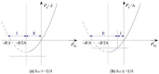
Figure 1.
The shape of h(ρ0ij) for A > 0.
Based on Figure 1, the equivalent correlation coefficient ρ0ij can be determined for A > 0 as follows:
To ensure that ρ0ij obtained from Equation (62) satisfies the definition of correlation coefficient (i.e., ), an applicable bound for ρij exists, i.e., , where ρij-max and ρij-min represent the upper and lower bounds, respectively.
When hext > −1/A (B2 − 4A < 0), i.e., that is, the interval of ρ0ij can be partitioned into two subintervals using the abscissas corresponding to ρ0ij = −B/2A, as illustrated in Figure 1b. If ρ0ij = −1 is in Interval I, the lower bound is determined as . On the other hand, if ρ0ij = −1 is in Interval II, the lower bound is to ensure . The lower bound for B2−4A < 0 can be expressed as .
When hext ≤ −1/A (B2 ≥ 4A), the interval of ρ0ij can be partitioned into two subintervals using the abscissas corresponding to ρij = −1, as depicted in Figure 1b. If ρ0ij = −1 is in Interval I, then the lower bound is determined to ensure . Conversely, if ρ0ij = −1 is in Interval II, the lower bound is set to ρij-min = −1. For B2 ≥ 4A, the lower bound can be expressed as .
Based on the previous discussion, if A > 0, the appropriate maximum value of the original correlation coefficient, which is equivalent to the lower bound of ρij, can be summarized as follows:
Substituting Equation (58) into the above Equation (63), the lower bound of ρij can be expressed as follows:
where
- (1)
- When A > 0, the upper bound of ρij can also be expressed as follows:then,
- (2)
- When A< 0, ρ0ij is determined by Equation (62), the applicable bound of ρij can be expressed as:
- (3)
- If A = 0, Equation (59) degenerates as a linear equation about ρ0ij as follows:
The applicable bound of ρij is given as follows:
6. Numerical Examples
6.1. Example 1: Computational Procedure with a Simplified Performance Function
Examine a cantilevered beam, as depicted in Figure 2, which is subjected to a uniformly distributed load (q) and possesses a beam length (l) of 4.0 m. The beam materials are characterized by Young’s modulus (E), while the inertia moment of the beam section is denoted by (I). The permissible deflection at the unattached extremity is 1/200 of the total beam length. As a result, the performance function can be formulated as follows:
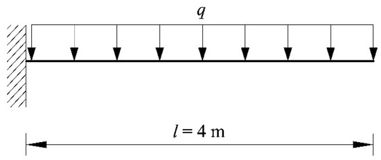
Figure 2.
Schematic diagram of the cantilevered beam.
The performance function, G(X), is articulated as a function encompassing three random variables: q, E, and I. The respective probability distributions and correlation matrix for these variables are presented in Table 3.
Table 3.
Random Variable Distributions and Correlation Matrix for Example 1.
6.1.1. Case 1: Structural Reliability with Correlated Variables
According to Equations (3)–(5) or Table 1, the first three L-moments of three random variables (q, E, and I) can be respectively given as follows:
Using Equations (25)–(27), the corresponding polynomial coefficients are given as follows:
Using Equation (58), the parameter matrix A can be obtained as follows:
Upon observation, it can be seen that all elements of A are greater than 0. Subsequently, by utilizing Equations (64) and (67), the upper and lower bounds of ρij can be expressed as follows:
The pertinent range of initial correlation coefficients matrix can be expeditiously procured as , which infers that the initial correlation matrix presented in this instance is suitable for the third L-moments transformation method. It is evident that the applicable range of the original correlation coefficient is sufficiently expansive, thereby rendering it satisfactory for a diverse array of general engineering problems.
Based on Equation (62), the equivalent correlation matrix is given as follows:
The Cholesky decomposition results of CZ can then be expressed as follows:
Assume initial checking point as:
The corresponding checking point in standard normal space can be readily obtained as using Equation (50). Subsequently, the initial reliability index β0 at u0 can be calculated as .
The Jacobian matrix at u0 can be evaluated using Equation (51) as follows:
Using Equation (52), the value of the performance function and gradient vector at the checking point u0 can be evaluated as follows:
Then, the next checking point u1 can be obtained based on Equation (53) as:
Then, the reliability index can be obtained as .
The absolute difference between β0 and β can be determined as:
Checking point in original space is determined as:
The above procedure is repeated using x1 as the new checking point until convergence is achieved. A comparison of results from different methods for Case 1 is presented in Table 4. The convergence criterion is met in five steps, resulting in a reliability index of βLM = 3.395 at the design point u* = (2.7039, −1.1539, −1.7016)T in standard normal space, which corresponds to the design point x* = (1627.03, 1.9415 × 10¹⁰, 3.3415 × 10⁻⁵)T in the original space.
Table 4.
Comparison of results by different methods for Case 1.
A comparative reliability analysis was conducted using the first three C-moments to perform the x-u and u-x transformations for the same example. The resulting reliability index, denoted as βCM, was obtained as 3.391 after convergence was achieved () in five steps. The corresponding design point in standard normal space was u* = (2.7031, −1.1527, −1.6949)T, and the corresponding design point in the original space was x* = (1633.32, 1.9376 × 10¹⁰, 3.3763 × 10⁻⁵)T.
Based on the available distribution information and initial correlation matrix of the random variables, the failure probability is determined to be 3.36 × 10⁻⁴ with a coefficient of variation of 3.77%, using the Monte Carlo simulation (MCS) approach with a sample size of 2 × 10⁶. The corresponding reliability index (βMCS) is found to be 3.397. Notably, the results obtained from the first three L-moments- and C-moments-based FORM approaches are found to be in close agreement with those obtained from MCS. It is noteworthy that the reliability index and failure probability ascertained via the L-moments method exhibit greater proximity to the values computed using the MCS method. This observation suggests that the L-moments approach yields superior accuracy in comparison to the C-moments method.
6.1.2. Case 2: Examining Random Variables with Greater Skewness
The proposed method, premised on the first three L-moments in Equation (16) and Equations (25)–(27), circumvents limitations on L-skewness, in contrast to the conventional third-moment standardization. If the coefficient of variation of q is 0.8, its skewness attains 2.924, which surpasses the scope of the third-moment transformation predicated on C-moments. In this scenario, the initial correlation matrix is verified with , facilitating reliability analysis based on L-moments. The acquired reliability index βLM = 1.266, converges to u* = (1.2429, −0.1334, −0.1972)T, corresponding to x* = (1963.9396, 2.0201 × 10¹⁰, 3.9149 × 10⁻⁵)T, after reaching convergence () in five steps. Utilizing MCS, the failure probability amounts to 9.272 × 10⁻2 (the coefficient of variation of MCS is 0.991%), with the corresponding reliability index of 1.319. It can be observed that FORM, based on L-moments, yields a result comparable to that of MCS, while FORM, based on C-moments, cannot be executed for this case.
Figure 3 illustrates the reliability indices in relation to the coefficients of variation of q, as determined using FORM based on L-moments and C-moments, along with the MCS results. Upon examining Figure 3, it becomes evident that the L-moments-based FORM results consistently demonstrate superior accuracy and alignment with the MCS outcomes, as compared to the C-moments-based FORM results, when the coefficients of variation of q range from 0.2 to 0.778.
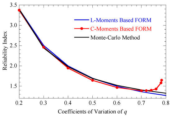
Figure 3.
Reliability indexes corresponding to coefficients of variation of q.
As the coefficients of variation of q exceed 0.778, the L-moments-based FORM continues to provide comparable results to those obtained through MCS, further emphasizing its advantageous performance. In contrast, the C-moments-based FORM becomes impractical, as the skewness of q surpasses the application range of the third-moment transformation predicated on C-moments. This observation accentuates the superior performance of the L-moments method compared to the C-moments method in the given context.
6.2. Example 2: Reliability Analysis with Unknown Probability Distribution
The second example encompasses a roof structure subjected to a uniformly distributed vertical load (qr), as delineated in Figure 4, which has been previously examined by [2]. The top cords and compression bars are composed of concrete, while the bottom cords and tension bars are constituted of steel. In the structural analysis, the uniformly distributed load (qr) was transformed into three nodal loads, each denoted as P = qrl/4. The serviceability limit state of the structure, with respect to its maximum vertical displacement, was considered. The performance function is expressed as follows:
where l represents the roof span, and the admissible deflection is arbitrarily fixed to 0.035 m. Furthermore, (Es, As) and (Ec, Ac) correspond to the Young’s modulus and cross-sectional areas of the steel and concrete beams, respectively. Table 5 consolidates the statistical information pertaining to the random variables.
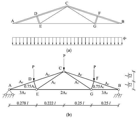
Figure 4.
The roof structure in example 2. (a) Schematic diagram of the roof structure, (b) Calculation diagram of the roof structure.
Table 5.
Random Variable Distributions and Sample L-moments for Example 2.
Assuming all random variables possess known CDFs/PDFs, the reliability index and failure probability can be effectively ascertained through the FORM procedure and MCS method. In order to examine the efficiency of the proposed approach, which incorporates random variables with unknown CDFs/PDFs, the CDFs/PDFs of random variables qr, l, As, Ac, Es, and Ec are considered unknown, with only a limited number of measured samples assumed to be known. Consequently, the first three sample L-moments can be calculated employing Equations (12)–(14) and Equation (15) and are presented in the rightmost section of Table 5. By utilizing the first three L-moments, the u-x and x-u transformations of the random variables can be seamlessly executed in accordance with Section 3. Subsequently, the reliability index and failure probability including random variables with unknown CDFs/PDFs, can also be readily obtained.
Upon examination of the available distribution information for the random variables, the failure probability is ascertained to be 1.96 × 10⁻⁴, accompanied by a coefficient of variation equal to 2.87%. This is achieved through the application of the MCS method, employing a sample size of 5 × 10⁶. The corresponding reliability index (βMCS) is determined to be 3.542. With respect to the known distribution information of random variables, the first-order reliability index (βFORM) is calculated as 3.679 using a general FORM procedure. In instances where distribution information remains unknown, the reliability index (βLM) computed by amalgamating FORM with merely the first three sample L-moments is 3.594.
It is worth noting that the results procured from the FORM approaches only based on the first three sample L-moments exhibit close alignment with those derived from MCS and the general FORM procedure. The comprehensive results acquired through the utilization of the CDFs/PDFs and the first three sample L-moments of qr, l, As, Ac, Es, and Ec are presented in Table 6. The table demonstrates that the checking points (in both original and standard normal spaces), the Jacobian for the last iteration, employing the first three sample L-moments of qr, l, As, Ac, Es, and Ec, exhibit a general proximity to those ascertained using the CDFs/PDFs of qr, l, As, Ac, Es, and Ec. This observation indicates that the first-order reliability index and calculation procedure, derived using exclusively the first three sample L-moments of random variables, exhibit substantial coherence with the index and calculation process ascertained via the CDFs/PDFs of random variables. This evidence not only reinforces the feasibility of the method proposed in this paper when the distribution of random variables is unknown but also accentuates its alignment with the scenarios encountered in engineering practice. Consequently, it encourages the promotion and application of the proposed method within real-world engineering contexts.
Table 6.
Comparisons of FORM Procedure Using Different Methods for Example 2.
6.3. Example 3: Reliability Analysis for Implicit Performance Functions
Consider a two-bay five-story frame structure subjected to lateral loads as depicted in Figure 5. The cross-sectional areas and moments of inertia of the frame members are listed in Table 7. The performance function is given as follows:
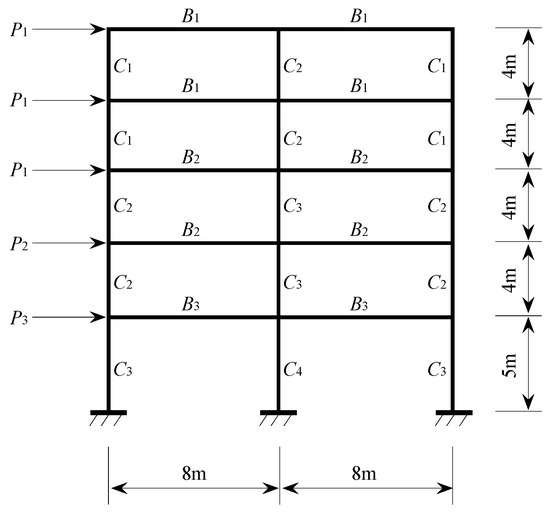
Figure 5.
Schematic Diagram of Two-bay five-story frame structure.
Table 7.
Probabilistic Characteristics of the Basic Random Variables.
The specified limit ulim = 0.055 m and the top-floor displacement u(X), which is determined by finite element analysis, are used in the following performance function. The correlation matrix of basic random variables is presented below:
The probabilistic characteristics and associated parameters of the random variables are presented in Table 7. The transformations from the standard normal space to the original space and vice versa are conducted for the random variables using Equations (45) and (50), respectively.
In this case, the boundary of the initial correlation matrix is examined to satisfy , thereby enabling the implementation of reliability analysis based on L-moments.
For the implicit performance function in this case, numerical differentiation methods can be utilized to determine the gradient vector . If the central difference method is employed, the expression for is given by:
where x0i (i = 1,2, …, n) represents the ith element of vector x0; and is the step size (generally chosen to be small enough as required).
Once the convergence is achieved (with ) in five steps, the reliability index can be easily determined as βLM = 2.209. Moreover, employing Monte Carlo simulation with known PDFs/CDFs and the initial correlation matrix, the reliability index can be calculated as βMCS = 2.215 (with corresponding failure probability Pf = 1.337 × 10⁻²) with high accuracy (coefficient of variation for Pf = 2.721%). Thus, the results obtained from the two methods in this example are almost identical.
7. Concluding Remarks
This study proposes a second-order polynomial normal transformation for structural reliability analysis based on the first three L-moments for both independent and correlated variables. The criteria for the admissible range of the initial correlation matrix have also been explored. Moreover, a FORM method has been developed based on the first three L-moments. Numerical examples are presented to investigate the accuracy and efficiency of the proposed method for structural reliability analysis. Several conclusions are drawn, as summarized in the following:
- (1)
- In practical engineering, the probability information of random variables is often incomplete, with access to only limited statistical data, rendering reliability calculations unfeasible. To address this issue, this paper presents an innovative solution. The proposed solution consists of two steps: first, employing the normal transformation and inverse transformation formulas based on the first three L-moments proposed in this paper, random variables can be approximated using polynomials containing standard normal random variables. Subsequently, after obtaining the approximate expressions for the random variables, the traditional FORM procedure is combined to calculate the reliability of the performance function using the approximate distribution and correlation matrix of the random variables. Several numerical examples provided, compared with the MCS method, demonstrate the feasibility and accuracy of the proposed method.
- (2)
- Although the normal transformation and inverse transformation of random variables can be achieved using C-moments, the accuracy of the C-moments-based FORM method tends to degrade as the coefficient of variation increases. When the coefficient of variation exceeds 0.778, the C-moments method becomes completely ineffective. In contrast, fortunately, the L-moments-based FORM method proposed in this paper consistently maintains agreement with the reliability indices calculated using the MCS method, regardless of the magnitude of the coefficient of variation. This is vividly illustrated in Case 2 of Example 2, which further demonstrates the broader applicability of the proposed method without being constrained by the coefficient of variation. It is worth mentioning that this paper also provides detailed boundary formulas and range justification for the equivalent correlation coefficients of the proposed method through mathematical derivation, further clarifying the applicability and scope of the new method.
- (3)
- In this study, a total of three numerical examples have been investigated to substantiate the feasibility, accuracy, and simplicity of the method proposed herein. These examples are grounded in real-world scenarios, encompassing a wealth of engineering contexts. They have been carefully selected to address diverse distribution types, multiple random variables, and intricate structural configurations from a variety of perspectives, underlining the extensive applicability of the presented method. Furthermore, the derived normal transformation and inverse transformation formulas for random variables, based on L-moments, are notably concise and straightforward. This simplicity not only facilitates comprehension among engineering practitioners but also promotes ease of implementation in real-life engineering problems. In light of these findings, it is recommended that the method proposed in this paper be further disseminated and applied within the engineering community. By doing so, it is anticipated that the method will contribute significantly to the advancement of structural reliability analysis and offer valuable insights for practitioners seeking to address complex engineering challenges.
Regarding future work, two primary research directions can be pursued to build upon the findings of this study. Firstly, a deeper investigation of the proposed method’s applicability to dynamic reliability analysis and more complex structural systems is needed. By extending the method to these domains, its versatility and robustness can be further established. Secondly, the exploration of alternative techniques that can substitute for normal transformation and inverse transformation is of interest, such as deep learning technologies. The potential integration of advanced machine learning algorithms with the proposed method could lead to enhanced performance and new insights into the field of structural reliability analysis.
By addressing these research avenues, the proposed method can continue to evolve and contribute to the advancement of structural reliability analysis and the resolution of complex engineering challenges.
Author Contributions
Conceptualization, Z.-P.L., D.-Z.H. and L.-W.Z.; Data curation, Y.S.; Formal analysis, Z.-P.L.; Funding acquisition, Z.-P.L. and L.-W.Z.; Investigation, Y.S.; Methodology, Z.-P.L., D.-Z.H. and L.-W.Z.; Resources, Z.Z. and Y.S.; Software, D.-Z.H. and L.-W.Z.; Supervision, Z.Z.; Validation, Z.-P.L. and L.-W.Z.; Writing—original draft, Z.-P.L.; Writing—review and editing, Z.-P.L., D.-Z.H. and L.-W.Z. All authors have read and agreed to the published version of the manuscript.
Funding
The authors gratefully acknowledge the support provided by the Natural Science Foundation of Changsha City (Grant No. kq2202234), the Natural Science Foundation of Hunan Province (Grant No. 2022JJ40188), the Excellent Youth Project of Hunan Provincial Department of Education, China Project (Grant No. 20B296), and the Fundamental Research Funds for the Central Universities of Central South University (2021zzts0225).
Data Availability Statement
There are no data available for sharing as it is confidential.
Conflicts of Interest
The authors affirm that they have no known financial or personal conflict of interest that may have influenced the findings or presentation of this paper.
References
- Melchers, R.E.; Beck, A.T. Structural Reliability Analysis and Prediction; John Wiley & Sons: Hoboken, NJ, USA, 2018. [Google Scholar]
- Zhao, Y.-G.; Zhang, X.-Y.; Lu, Z.-H. Complete monotonic expression of the fourth-moment normal transformation for structural reliability. Comput. Struct. 2018, 196, 186–199. [Google Scholar] [CrossRef]
- Echard, B.; Gayton, N.; Lemaire, M.; Relun, N. A combined importance sampling and kriging reliability method for small failure probabilities with time-demanding numerical models. Reliab. Eng. Syst. Saf. 2013, 111, 232–240. [Google Scholar] [CrossRef]
- Dang, C.; Wei, P.; Song, J.; Beer, M. Estimation of failure probability function under imprecise probabilities by active learning–augmented probabilistic integration. ASCE-ASME J. Risk Uncertain. Eng. Syst. Part A Civ. Eng. 2021, 7, 04021054. [Google Scholar] [CrossRef]
- Zheng, Z.; Dai, H.; Beer, M. Efficient structural reliability analysis via a weak-intrusive stochastic finite element method. Probabilistic Eng. Mech. 2023, 71, 103414. [Google Scholar] [CrossRef]
- Aldosary, M.; Cen, S.; Li, C. Hermite polynomial normal transformation for structural reliability analysis. Eng. Comput. 2021, 38, 3193–3218. [Google Scholar]
- Zhou, W.; Gong, C.; Hong, H.P. New perspective on application of first-order reliability method for estimating system reliability. J. Eng. Mech. 2017, 143, 04017074. [Google Scholar] [CrossRef]
- Huang, X.; Li, Y.; Zhang, Y.; Zhang, X. A new direct second-order reliability analysis method. Appl. Math. Model. 2018, 55, 68–80. [Google Scholar] [CrossRef]
- Zhang, L.-W.; Dang, C.; Zhao, Y.-G. An efficient method for accessing structural reliability indexes via power transformation family. Eng. Syst. Saf. 2023, 233, 109097. [Google Scholar] [CrossRef]
- Chen, W.; Gong, C.; Wang, Z.; Frangopol, D.M. Application of first-order reliability method with orthogonal plane sampling for high-dimensional series system reliability analysis. Eng. Struct. 2023, 282, 115778. [Google Scholar] [CrossRef]
- Yu, D.; Ghadimi, N. Reliability constraint stochastic UC by considering the correlation of random variables with Copula theory. IET Renew. Power Gener. 2019, 13, 2587–2593. [Google Scholar] [CrossRef]
- Chen, C.; Wu, W.; Zhang, B.; Sun, H. Correlated probabilistic load flow using a point estimate method with Nataf transformation. Int. J. Electr. Power Energy Syst. 2015, 65, 325–333. [Google Scholar] [CrossRef]
- Xiao, Q. Evaluating correlation coefficient for Nataf transformation. Probabilistic Eng. Mech. 2014, 37, 1–6. [Google Scholar] [CrossRef]
- Hu, Z.; Mansour, R.; Olsson, M.; Du, X. Second-order reliability methods: A review and comparative study. Struct. Multidiscip. Optim. 2021, 64, 3233–3263. [Google Scholar] [CrossRef]
- Madsen, H.O.; Krenk, S.; Lind, N.C. Methods of Structural Safety; Courier Corporation: New York, NY, USA, 2006. [Google Scholar]
- Zhao, Y.-G.; Lu, Z.-H.; Ono, T. A simple third-moment method for structural reliability. J. Asian Arch. Build. Eng. 2006, 5, 129–136. [Google Scholar] [CrossRef]
- Lu, Z.-H.; Cai, C.-H.; Zhao, Y.-G. Structural reliability analysis including correlated random variables based on third-moment transformation. J. Struct. Eng. 2017, 143, 04017067. [Google Scholar] [CrossRef]
- Ulrych, T.J.; Velis, D.R.; Woodbury, A.D.; Sacchi, M.D. L-moments and C-moments. Stoch. Environ. Res. Risk Assess. 2000, 14, 50–68. [Google Scholar] [CrossRef]
- Withers, C.S.; Nadarajah, S. Bias-reduced estimates for skewness, kurtosis, L-skewness and L-kurtosis. Stat. Plan. Inference 2011, 141, 3839–3861. [Google Scholar] [CrossRef]
- Sankarasubramanian, A.; Srinivasan, K. Investigation and comparison of sampling properties of L-moments and conventional moments. J. Hydrol. 1999, 218, 13–34. [Google Scholar] [CrossRef]
- Zhang, L.-W.; Lu, Z.-H.; Zhao, Y.-G. Dynamic reliability assessment of nonlinear structures using extreme value distribution based on L-moments. Mech. Syst. Signal Process. 2021, 159, 107832. [Google Scholar] [CrossRef]
- Gao, S.; Zheng, X.Y.; Huang, Y. Hybrid C-and L-Moment–based Hermite transformation models for non-Gaussian processes. J. Eng. Mech. 2018, 144, 04017179. [Google Scholar] [CrossRef]
- Tong, M.-N.; Zhao, Y.-G.; Zhao, Z. Simulating strongly non-Gaussian and non-stationary processes using Karhunen–Loève expansion and L-moments-based Hermite polynomial model. Mech. Syst. Signal Process. 2021, 160, 107953. [Google Scholar] [CrossRef]
- Zio, E.; Zio, E. Monte Carlo Simulation: The Method; Springer: Berlin/Heidelberg, Germany, 2013. [Google Scholar]
- Betz, W.; Papaioannou, I.; Straub, D. Bayesian post-processing of Monte Carlo simulation in reliability analysis. Reliab. Eng. Syst. Saf. 2022, 227, 108731. [Google Scholar] [CrossRef]
- Chen, X.; Tung, Y.-K. Investigation of polynomial normal transform. Struct. Saf. 2003, 25, 423–445. [Google Scholar] [CrossRef]
- Ji, X.; Huang, G.; Zhang, X.; Kopp, G.A. Vulnerability analysis of steel roofing cladding: Influence of wind directionality. Eng. Struct. 2018, 156, 587–597. [Google Scholar] [CrossRef]
Disclaimer/Publisher’s Note: The statements, opinions and data contained in all publications are solely those of the individual author(s) and contributor(s) and not of MDPI and/or the editor(s). MDPI and/or the editor(s) disclaim responsibility for any injury to people or property resulting from any ideas, methods, instructions or products referred to in the content. |
© 2023 by the authors. Licensee MDPI, Basel, Switzerland. This article is an open access article distributed under the terms and conditions of the Creative Commons Attribution (CC BY) license (https://creativecommons.org/licenses/by/4.0/).