Article

Embodied Carbon Minimization for Single-Story Steel Gable Frames

1
Structural Engineering Department, Zagazig University, Zagazig 44519, Egypt
2
Civil Engineering, Southern Illinois University Edwardsville, Edwardsville, IL 62026, USA
*
Author to whom correspondence should be addressed.
Buildings 2023, 13(3), 739; https://doi.org/10.3390/buildings13030739
Submission received: 23 February 2023 / Revised: 7 March 2023 / Accepted: 10 March 2023 / Published: 11 March 2023
(This article belongs to the Section Building Structures)

Abstract

:
As the construction industry, especially steel construction, contributes to a large portion of global greenhouse gas emissions, sustainable structural design has become a necessity to achieve the world vision of reaching net zero emissions by 2050. As steel portal frames are the most used structural system for single-story buildings, the main objective of this study is to determine the optimal steel portal frame configuration using prismatic and/or non-prismatic members to achieve the least embodied carbon. Five different portal frame configurations are considered under the effect of five distinct loading conditions. The results led to developing design charts consisting of contour plots showing the embodied carbon per unit of volume enclosed by the steel frame for different frame configurations, loading conditions, span lengths, and column heights. In addition, by increasing the number of member divisions, design variables, and non-prismatic segments, the average embodied carbon of the steel portal frames can be significantly reduced by about 14.34% up to 26.47% relative to the configuration with only prismatic members.

1. Introduction

Over the past few centuries, human life activities, especially the Industrial Revolution, have cumulatively impacted our planet, causing drastic changes in our climate [1]. Climate change represents a great danger to human life on Earth as it drives an increase in the intensity and frequency of heat waves, droughts, hurricanes, and other natural disasters [2,3,4,5]. The burning of fossil fuels as energy resources led to the increase in the concentration of greenhouse gases (GHGs), including carbon dioxide (CO 2 ), methane (CH 4 ), and nitrous oxide (N 2 O), in the Earth’s atmosphere, causing an increase in the average temperature of the Earth’s surface, which is known as global warming [6,7,8]. Scientists forecast that if the environmentally harmful practices continue, the average temperature of the Earth’s surface will increase by 2–6 ° C by the end of the 21st century using 3 different CO 2 emission scenarios [6]. Therefore, it is our responsibility to control GHGs emissions in every possible way. Many countries have recently established legal commitments [9] to cut down their CO 2 emissions to meet the global target of a 45% reduction in CO 2 emissions by 2030 and achieve net-zero carbon emissions by 2050 [10]. However, a significant mismatch between the global aspirations and current global CO 2 emissions can be clearly noted [11].
According to United Nations Global Status Report (GSR), the building and construction industry is a major source of GHGs emissions as it contributes to more than 37% of energy- and process-related CO 2 emissions and over 34% of energy demand globally [12]. Therefore, assessing and minimizing the CO 2 emissions associated with the construction industry have attracted significant attention in the scientific research community. There are two main types of CO 2 emissions related to the construction industry: operational carbon and embodied carbon. Operational carbon is the carbon associated with the energy consumed during various building operations, including heating, cooling, lighting, etc. Embodied carbon is the carbon emissions associated with material extraction, fabrication, transportation to site, construction, maintenance, and demolition [12]. Today, operational carbon surpasses embodied carbon in the contribution to the total CO 2 emissions from the construction industry [13]. However, as the world utilizes more sources of renewable energy [14], the contribution of operational carbon is beginning to decline compared with embodied carbon, making it an important target to be minimized [15,16].
Several studies have been conducted on the life cycle assessment (LCA) of both carbon and energy associated with buildings [17,18,19], whereas other researchers have focused primarily on assessing embodied carbon [20,21,22,23,24]. Pomponi and Moncaster reviewed the literature encompassing various measures that can be used to mitigate and reduce the embodied carbon of the built environment [24]. One of the mitigation measures they proposed is to make better design decisions during the preliminary design stage where a significant reduction in embodied carbon can be achieved [24]. Targeting embodied carbon emissions at this stage opens the field for optimization researchers to contribute to the global target of reducing carbon emissions.
The three main construction materials used in most building projects are reinforced concrete, steel, and timber [25,26,27]. According to the Allwood et al. investigation [28], the steel industry alone contributes approximately 2.5 gigatonnes of CO 2 emissions, which is about 25% of the total global CO 2 emissions. Nearly half of the produced steel is utilized in the construction industry [28]. Therefore, extensive scientific effort should be focused on minimizing the GHG emissions produced by the steel construction industry to effectively control global warming and climate change [28]. Steel portal frames are one of the most commonly used structural systems to cover medium to large spans due to their efficiency and ease of fabrication and erection [29,30,31]. For example, in the United Kingdom, steel portal frames are used in about 90% of single-story commercial buildings [32]. Therefore, making these structures net-zero carbon can significantly contribute to reducing CO 2 emissions worldwide [33].
In prior literature, there is a wealth of research optimizing the cost and weight of steel portal frames as, traditionally, the steel cost is the most important element structural engineers try to minimize [30,34,35,36,37,38,39,40,41,42]. As the world focus shifts toward more sustainable structural designs, however, researchers are focusing more on minimizing the carbon content of steel buildings than on cost savings. McKinstray et al. developed a methodology combining both a multi-objective evolutionary algorithm and artificial neural networks to minimize the carbon emissions of single-story steel commercial buildings [43]. They concluded that asymmetric frame configurations are necessary to achieve the highest carbon offset using photovoltaic (PV) panels installed on the south-facing roof direction. In addition, it was found that carbon offsetting is more and more challenging, and in some instances impossible, for buildings with big volumes caused by high eaves. It was also discovered that the use of asymmetric geometries enabled lower embodied energy structures with similar carbon efficiency. D’Amico and Pomponi introduced a software tool on Rhino Python that can be used to minimize both steel mass and carbon emissions of steel-framed buildings using the sequential search (SS) algorithm [25]. McKinstray et al. utilized the well-regarded genetic algorithm (GA) to compare the optimal weights of various frame configurations, utilizing rolled, fabricated, and tapered sections [33]. They concluded that utilizing fabricated and tapered members in steel portal frames can achieve material savings up to 9% and 11%, respectively, compared to using hot-rolled sections. However, they considered only one configuration of steel frames consisting of six tapered members. In addition, they considered neither snow loads nor seismic loads. In addition, they concluded that an asymmetric structural shape would add 5–13% more weight on average, with extra PV loading having little to no impact on the ideal design. Our review of the current literature identified that there is a lack of studies comparing the embodied carbon emissions of different configurations of steel portal frames with tapered members under all practical load types.
Hoping to add to the current literature, the main contributions of this study are to compare the embodied carbon of four different practical tapered steel portal frame configurations against that of prismatic sections to determine the most environmentally sustainable design for different span lengths, column heights, and loading conditions and to determine the optimal span length and column height range that require the least embodied carbon per unit of enclosed steel frame volume.

2. Optimization Problem Formulation

In this section, a detailed description of the optimization problem formulation is presented.

2.1. Objective Function

The embodied carbon, which can be estimated by global warming potential (GWP) [44], is considered the objective function of this optimization process. In this study, the `cradle-to-cradle’ approach is utilized by considering the embodied carbon emissions over the entire life cycle of the building. This approach includes the initial stage (Modules A1 to A5), the use stage (Modules B1 to B7), the end-of-life stage (Modules C1 to C4), and the recovery or recycling potential of the materials (Module D). In this study, the embodied carbon in-use (Modules B1 to B5) and operational carbon impact (Modules B6 to B7) are not considered because the embodied carbon of the use stage is identical for all of the compared steel frame models. Therefore, it does not affect the choice of the optimal steel frame configuration. The objective function is given by Equation (1) as follows:
G W P = i = 1 N e l . j = 1 N m o d . E C C j · ρ L i 1 2 t w i ( h w 1 i + h w 2 i ) + 2 b f i t f i
where N e l . is the number of frame elements; ρ is the steel density; L i is the member length; t w i , h w 1 i , and h w 2 i are the web plate thickness, height at the beginning, and height at the end, respectively; t f i and b f i are the flange plate thickness and width, respectively; N m o d . is the number of considered embodied carbon modules; and E C C j is the embodied carbon coefficient of Module j for the fabricated steel beams utilized for the frame members. The embodied carbon coefficients calculated by Drewniok et al. [45] for each module are utilized in this study.

2.2. Design Variables

The optimized frames cover a single span with a variable length ranging between 10 m and 50 m with a step of 10 m (5 different span lengths). The height of the column is also variable, ranging between 6 m and 16 m with a step of 2 m (6 distinct column heights). The cross-sectional dimensions of the steel members are considered the sizing design variables. Here, t f c , b f c , t w c , h w c i , and h w c j are the column flange plate thickness, width, column web plate thickness, bottom height, and top height, respectively, and t f r , b f r , t w r , h w r i , and h w r j are the rafter flange plate thickness, width, rafter web plate thickness, middle height, and edge height, respectively. In some frame configurations, specific members are subdivided into segments. The ratio between the segment length to the total member length is defined as the segment length ratio (SLR). For the shape optimization, the span length, column height, and segment length ratios of both the columns ( S L R c ) and the rafter ( S L R r 1 and S L R r 2 ) are considered geometry design variables. Finally, for the topology optimization, five different configurations of steel gable frames incorporating prismatic and/or non-prismatic sections are optimized as shown in Figure 1 (where the number between the parentheses represents the design variable number). The number of design variables for the control model, Models 1, 2, 3, and 4, are 8, 10, 14, 14, and 16, respectively. The possible values for each design variable are presented in Table 1.

2.3. Design Constraints

In order to obtain practical optimal designs that can represent the common engineering practice, ANSI/AISC 360-16 [46], ANSI/AISC 341-16 [47], ASCE/SEI 7-16 [48], and Design Guide 25 [49] provisions are utilized to establish the strength constraints and serviceability constraints of the optimization problem as given in Table 2 and Table 3, respectively. P u , P c , M u x , M c x , M u y , and M c y are the factored axial force, design axial strength, factored bending moment about the major axis, design moment capacity about the major axis, factored bending moment about the minor axis, and design moment capacity about the minor axis, respectively. This constraint is used to control the in-plane resistance and out-of-plane resistance at purlins and bracing points locations. Here, δ v is the vertical displacement of the apex, L is the span length, δ h is the horizontal displacement of the eave, h is the mean roof height of the frame, and δ M is the seismic drift as defined in ASCE/SEI 7-16 [48].

2.4. Penalty Function

To improve the algorithm’s ability to balance between exploration at the start of the optimization process and exploitation at the end of it, the S-shape penalty function proposed by Liu et al. [50] is adopted to calculate the penalized objective function of the frame. The function is defined by Equation (2) as follows:
P ( i t e r ) = 10 θ 2 θ 1 1 + e 20 ( i t e r + N 4 ) N + θ 1
where i t e r and N are the iteration and the total number of iterations, respectively, and θ 1 and θ 2 are parameters that control the bounds of the penalty function. The penalty function varies between [ 10 θ 1 , 10 θ 2 ] . In this study, the values of θ 1 and θ 2 are taken as zero and three, respectively.

3. Structural Analysis

Structural analysis is performed on MATLAB software [51] using the assembly stiffness method according to Equation (3) as follows:
{ D } n × 1 = K g n × n 1 { F } n × 1
where { D } n × 1 is the displacement vector, K g n × n is the structure (global) stiffness matrix, { F } n × 1 is the applied loads vector, and n is the number of degrees of freedom in the structure. Each tapered member is modeled using the stepped representation as permitted by the Design Guide 25 [49]. In order to avoid the occurrence of shear locking and ill-conditioned stiffness matrices [52], the stiffness matrix for each element is derived based on the Timoshenko beam element stiffness matrix presented in Equations (4)–(6) as:
k e = E · A / L 0 0 E · A / L 0 0 0 η / L η / 2 0 η / L η / 2 0 η / 2 η ( 4 + ζ ) L / 12 0 η / 2 η ( 2 ζ ) L / 12 E · A / L 0 0 E · A / L 0 0 0 η / L η / 2 0 η / L η / 2 0 η / 2 η ( 2 ζ ) L / 12 0 η / 2 η ( 4 + ζ ) L / 12
with
η = 12 E · I x ( 1 + ζ ) L 2
ζ = 12 E · I x · k A · G · L 2
where G is the shear modulus, and k is the shear correction factor proposed by Cowper [53], which is defined by Equations (7) and (8) as:
k = 10 ( 1 + ν ) ( 1 + 3 ω ) 2 γ
γ = 12 + 72 ω + 150 ω 2 + 90 ω 3 + ν ( 11 + 66 ω + 135 ω 2 + 90 ω 3 ) + 30 μ 2 · ω ( 1 + ω ) + 5 ν · η 2 · ω ( 8 + 9 ω )
where ω is equal to ( 2 b · t f ) / ( h · t w ) , μ is calculated as b / h , and ν is the Poisson’s ratio.
In order to calculate the in-plane buckling strength of tapered members, the successive approximations method is utilized according to Design Guide 25 provisions [49]. The elastic buckling multiplier ( γ e ), defined as the ratio of the elastic buckling load to an arbitrarily chosen reference load P r e f as shown in Equation (9), is calculated and used to estimate the elastic buckling load P e of tapered members.
γ e = P e P r e f
As recommended by ANSI/AISC 360-16 specifications [46], the direct analysis method is used to account for the inelastic effects. In addition, the second-order effects (i.e., P Δ and P δ effects) are accounted for using the amplified first-order analysis approach as permitted by ANSI/AISC 360-16 specifications [46].

4. Structural Loading

In this section, the methodology of loading the optimized frames is briefly presented.

4.1. Loading Methods

The provisions of ASCE/SEI 7-16 [48] are utilized to establish the structural loading of the optimized frames. The dead load on the frame encompasses the own weight of the steel members in addition to a superimposed dead load of 250 N/m 2 to account for the weight of purlins and roofing material in addition to any other collateral loads. The minimum live load for pitched roofs is 960 N/m 2 (20 psf). For the snow load, both the balanced and unbalanced distribution of snow loads are considered in this study. As all the considered frames can be classified as low-rise buildings, the envelope procedure for wind load calculation is utilized. The equivalent lateral force approach for seismic load calculation is adopted in this study for both the horizontal and vertical components of the seismic load. Notional loads are calculated as per ANSI/AISC 360-16 specifications [46].
All the parameters necessary to calculate the applied loads according to ASCE/SEI 7–16 provisions [48] are given in Table 4, Table 5 and Table 6 for the snow load, wind load, and seismic load, respectively.

4.2. Loading Conditions

In order to investigate the effect of different load types on the embodied carbon of steel frames, five distinct locations in the United States with very different loading conditions are considered for the loading of the optimized frames. St. Charles represents high seismic loads, whereas Miami represents high wind loads. Detroit, St. Paul, and Berlin are selected to represent the snow load variation from low to medium to high, respectively. The different loading parameters that depend on the frame location are presented in Table 7, where P g is the ground snow load, V is the basic wind speed, and the different seismic parameters are defined in ANSI/AISC 360-16 provisions [46]. The load combinations provided by ASCE/SEI 7-16 specifications [48] are adopted in this study.

5. The Optimization Process

In this section, a brief description of the optimized building characteristics, material properties, and the utilized optimization algorithm is presented.

5.1. Utilized Building Configuration

The considered frame is supported by two hinges. The thickness of the roofing layer is considered equal to 0.20 m. The maximum purlin spacing is considered equal to 2.50 m. A total of 5 different span lengths (L) are considered to determine the optimal span length causing the least embodied carbon, including 10, 20, 30, 40, and 50 m. In addition, 6 different eave heights ( H e a v e ) including 6, 8, 10, 12, 14, and 16 m are utilized in this study. The roof slope of the gable frame is considered equal to 17.5% (for typical steel industrial buildings).

5.2. Utilized Material Properties

For the steel structural members, carbon steel of grade ASTM A36 as per ANSI/AISC 360-16 specifications [46] is utilized with the following material properties: ρ = 7850 Kg/m 3 , F u = 400 MPa, F y = 250 MPa, ν = 0.3 , E = 200 GPa, and G = 79.3 GPa, where ρ is the steel density, F u is the ultimate strength, F y is the yield strength, ν is the Poisson ratio, E is the modulus of elasticity, and G is the shear modulus.

5.3. Utilized Optimization Algorithm

Many robust and highly efficient meta-heuristic optimization algorithms have been recently developed to optimize practical engineering problems. A new meta-heuristic optimization algorithm called the crystal structure algorithm (CryStAl) was proposed by Talatahari et al. [54]. In this study, an adaptation of CryStAl is utilized for minimizing the embodied carbon. The optimization process utilizes 100 iterations and 50 search agents.

6. Results and Discussion

In this section, the results obtained by performing more than 3.8 million frame analyses using the MATLAB program [51] written by the authors are discussed and analyzed.

6.1. Minimizing the Embodied Carbon of Different Frame Configurations

A sample of the optimal steel frame designs and their associated GWP for a specific frame located in Detroit with a span length of 20 m and a column height of 8 m is presented in Table 8. As shown by the results, Model 4 managed to achieve the highest reduction in the embodied carbon (EC) by about 26.18% compared to the control model. Models 2 and 3 followed Model 4 by achieving an EC reduction of about 25.75% and 23.07%, respectively, compared to the control model. Although Model 1 performed the worst among different configurations of steel frames with tapered members, it still managed to achieve a significant EC reduction compared to the control model, with only prismatic members, by about 12.23%. In order to compare the EC of frames with various span lengths and column heights, the steel frame embodied carbon, measured by kgCO 2 , is divided by the volume of space enclosed by the steel frame, measured by m 3 , to obtain the embodied carbon per unit of the enclosed volume, measured by kgCO 2 /m 3 . Relating the carbon emissions to the building volume is commonly utilized in environmental engineering, especially for assessing the regulated carbon emissions caused by heating, cooling, and ventilation which are directly related to the building volume [43]. In addition, if a project requires a specific enclosed volume (e.g., for a storage facility), the span length and column height corresponding to the least embodied carbon per unit volume can be utilized to achieve the minimum total embodied carbon. In the rest of this study, the embodied carbon per unit volume will be denoted by the embodied carbon intensity (ECI).
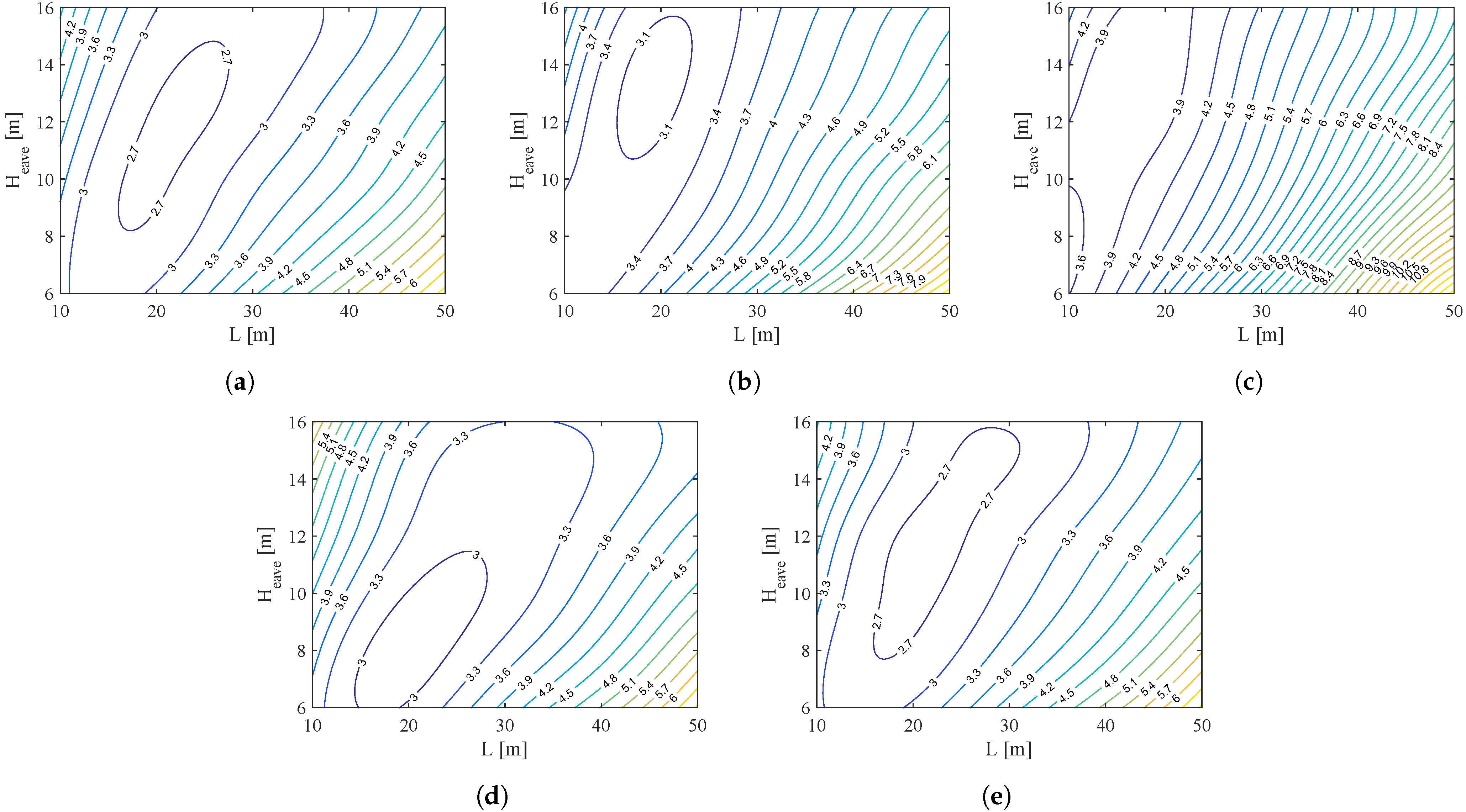
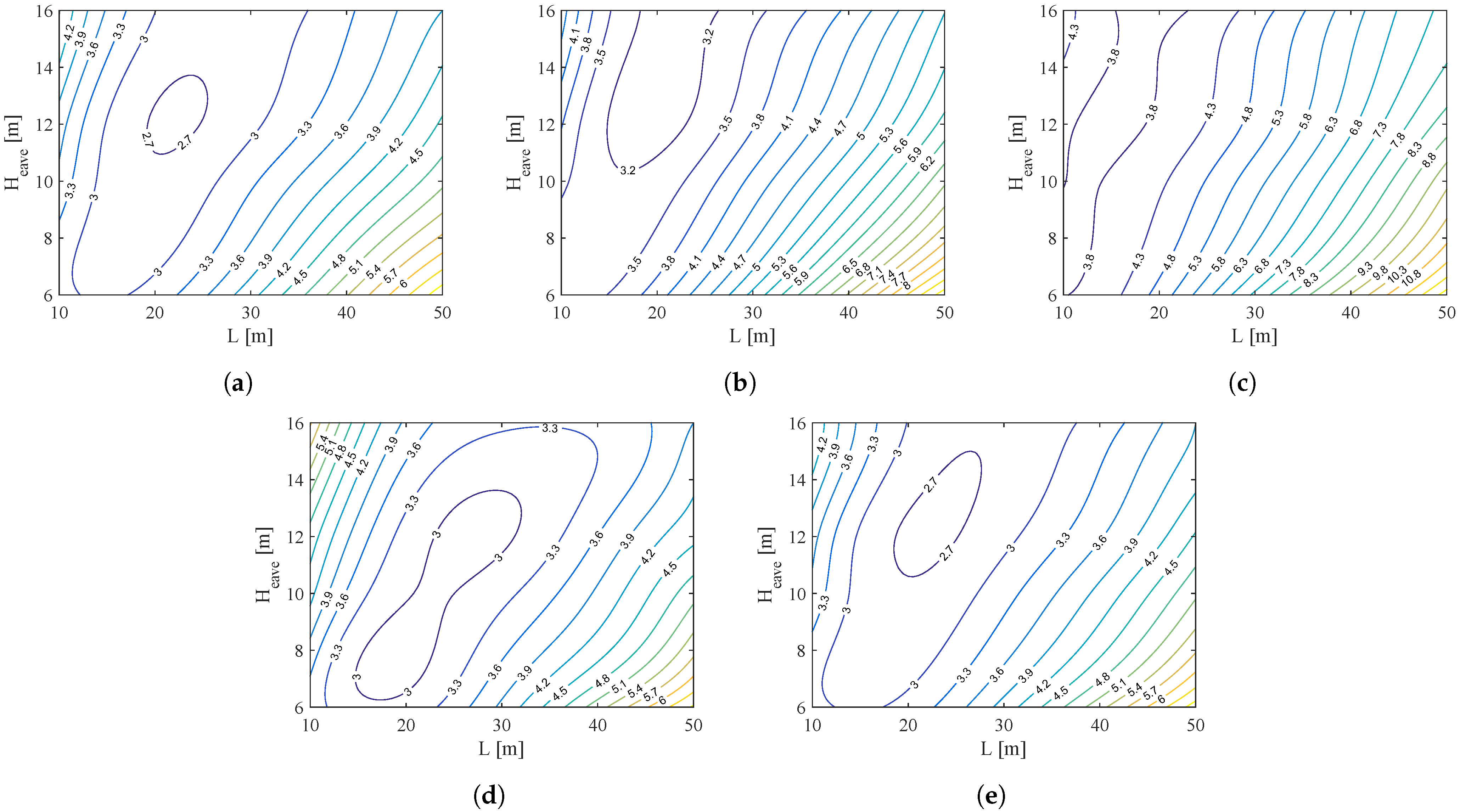
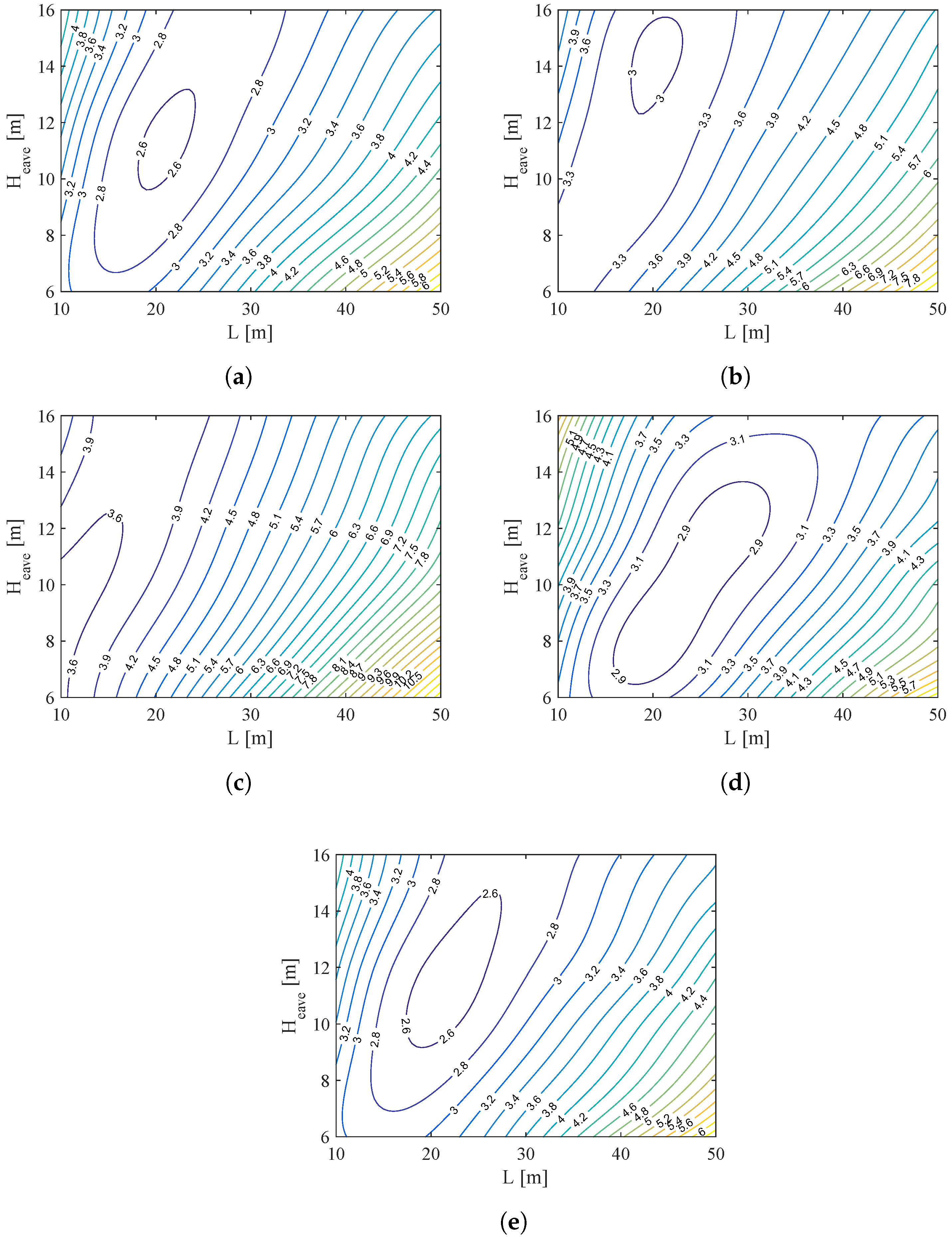
Contour plots showing the ECI corresponding to different span lengths (L) and column heights (H e a v e ) for different frame models were prepared. As noticed by the results in Table 8, Model 4 managed to achieve the least embodied carbon, so its contour plots are presented in Figure 2, whereas the contour plots of the remaining models are presented in Appendix A.
For a specific loading condition, for example Detroit (shown in Figure 2a), the optimal span length and column height, giving ECI of less than 2.6 kgCO 2 /m 3 of the enclosed volume, are between 18 m and 24 m for the span length and between 9.6 m and 13.2 m for the column height. Therefore, the optimal span length and column height ranges can be determined for different loading conditions and frame models using these contour plots. Note that in the highest snow load case (in Berlin, NH) shown in Figure 2c, the optimal span length range (between 10 m and 17 m) is much shorter than the optimal range for the previously discussed case of Detroit (between 18 m and 24 m). This is mainly due to the higher snow load that causes, in the case of larger spans, higher vertical deflections and straining actions, resulting in larger required steel sections and higher embodied carbon. Another observation is that the minimum ECI associated with Berlin (3.47 kgCO 2 /m 3 ) is much more than that of Detroit (2.58 kgCO 2 /m 3 ) with about a 34.5% increase. This shows the high sensitivity of steel frames to higher snow loads. These contour plots can be utilized as a design aid to obtain the ECI of a steel gable frame with any span length, column height, loading condition, and frame configuration.
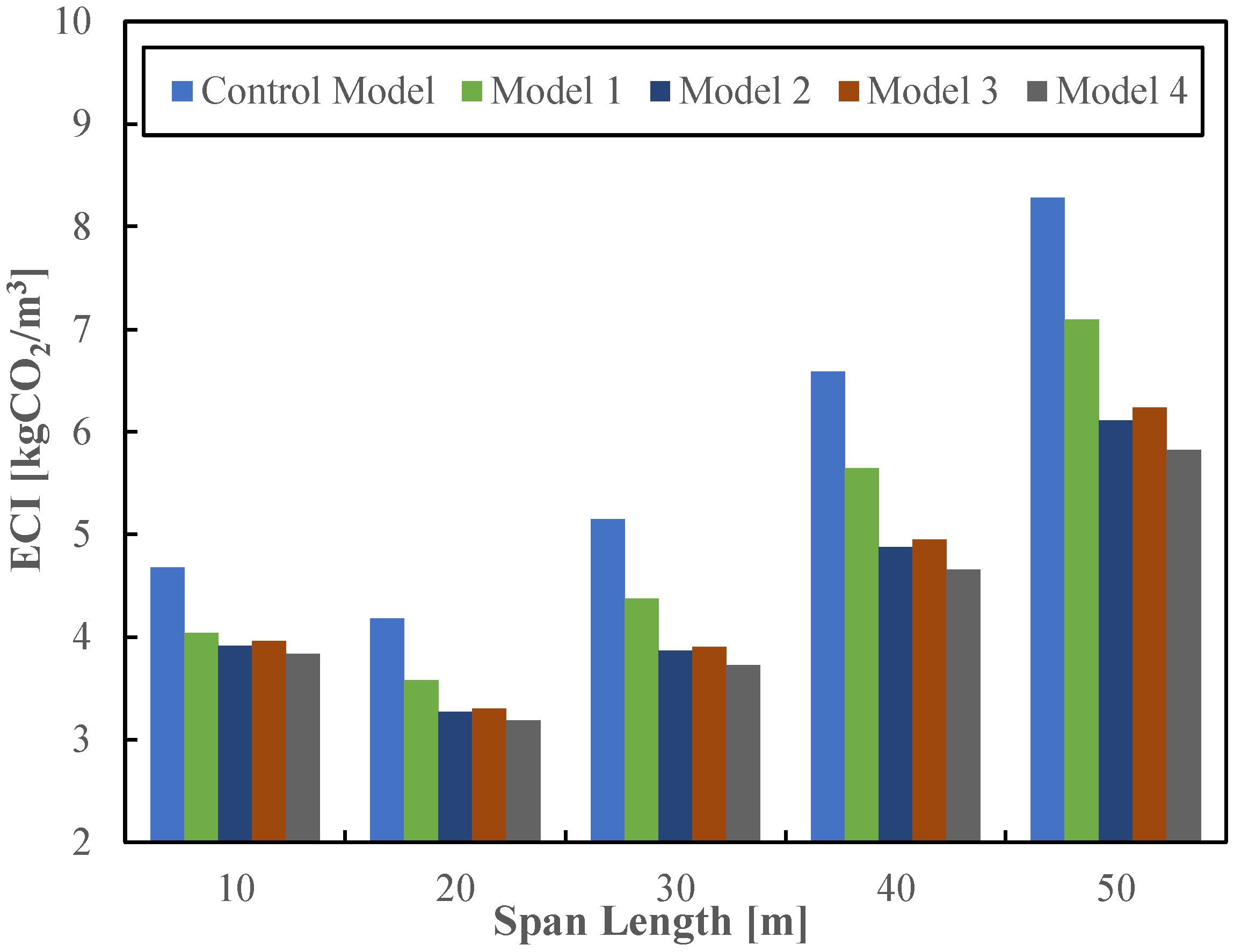
To determine the variation trend of the ECI with the span length, the average ECI for each model for different span lengths is shown in Figure 3. It is shown that all the models achieved the least ECI when utilizing a short-to-medium span length (i.e., 20 m). As the span length increases above 20 m, the ECI significantly increases. Therefore, frames with large span lengths are not optimal when the objective is to minimize the embodied carbon emissions. On the other hand, frames with spans less than 20 m have higher ECI, mainly due to the small volume enclosed by the frames compared to the required amount of steel for the frame members.
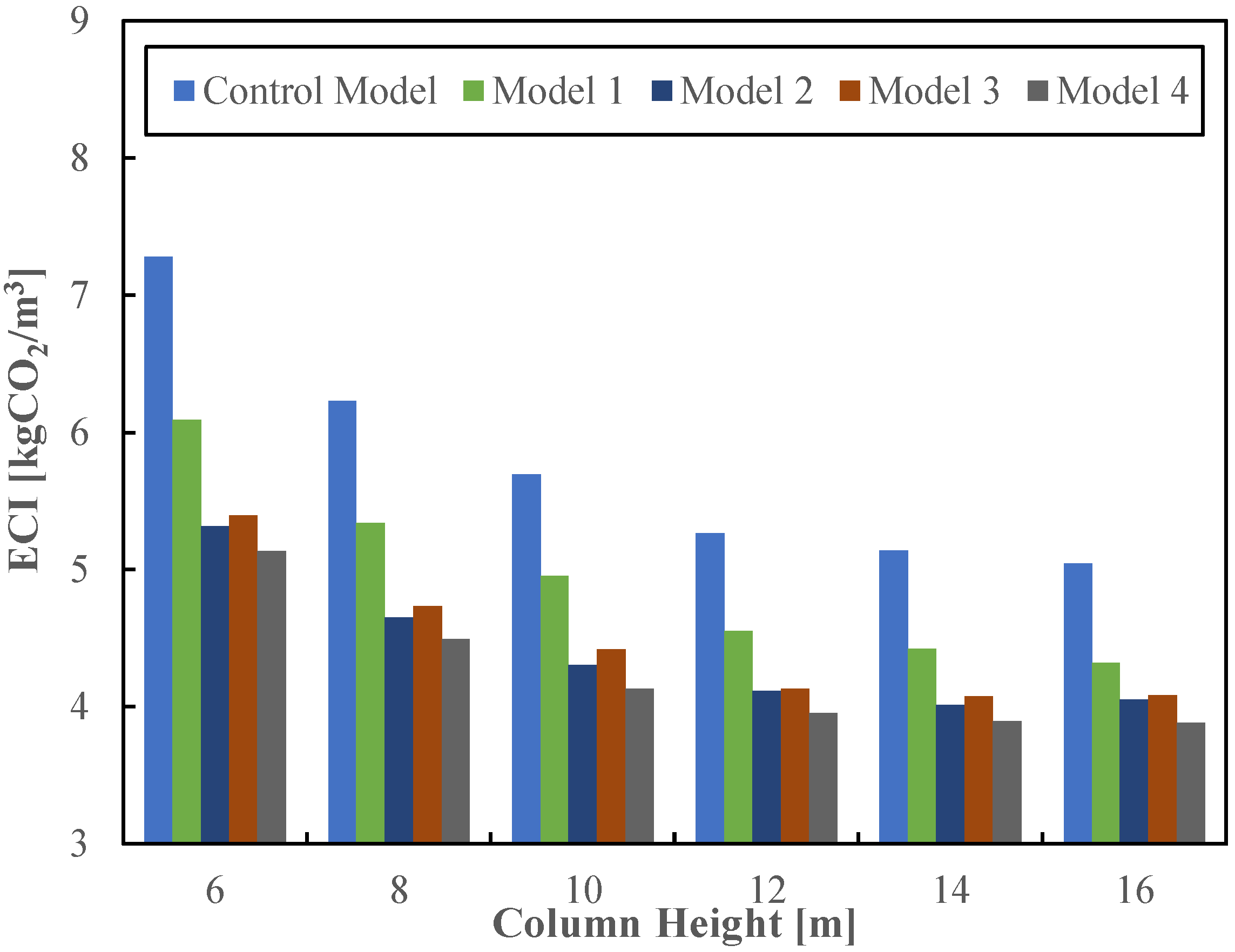
To investigate the ECI variation with the column height, the average ECI variation for different models with different column heights is presented in Figure 4. Note that for all the models, as the column height increases, the average ECI decreases. This can be explained by the higher rate of volume increase due to increasing the column height compared to the embodied carbon increase rate. However, increasing the column height to reduce the ECI has diminishing returns, as shown in Figure 4, as the reduction seems to be negligible for column heights greater than 12 m. This is mainly due to the higher wind loads associated with larger column heights, leading to requiring a larger amount of steel and thus a larger amount of embodied carbon. Therefore, to achieve the least embodied carbon per unit of enclosed volume while keeping the total embodied carbon at a reasonable level, medium column heights (i.e., about 12 m) are recommended.

6.2. Comparison of Different Gable Frame Configurations

In order to visualize the contribution of the embodied carbon resulting from each specific module (A, C, and D), Figure 5 shows the average ECI of each module for different frame models.
The ECI results of the control model are discussed in detail as a case study. Module A1, representing the process of extraction and supply of raw materials, has the largest contribution to the ECI of steel gable frames which is equal to 11.42 kgCO 2 /m 3 , representing about 75.3% of the total positive embodied carbon of the steel gable frame. The second largest contributor to positive embodied carbon is Module A3, which represents the embodied carbon caused by the manufacturing processes of the steel frame members using steel plates. Module A3 contributes to the total positive embodied carbon of steel gable frames by about 2.49 kgCO 2 /m 3 (about 16.5%). As can also be noted from Figure 5, both the construction process stage (Modules A4 and A5) and end-of-life and demolition stage (Modules C1 to C4) only contribute a small fraction to the total positive embodied carbon of the steel gable frame of about 0.26 kgCO 2 /m 3 (1.7%) and 0.69 kgCO 2 /m 3 (4.5%), respectively. As structural steel is a highly recyclable material, Module D (representing the reuse, recovery, or recycling potential of steel) represents a negative contribution to the embodied carbon by offsetting the positive embodied carbon by about 4.63 kgCO 2 /m 3 (about 30.6% of the positive embodied carbon over the entire life cycle of the material). After investigating the contribution of each module in the entire life cycle embodied carbon of different steel frames, Table 9 gives the percentage of the overall achieved reduction in the ECI of Models 1, 2, 3, and 4 compared to the control model that uses only prismatic members.
As shown in Table 9, Model 4 achieved the highest ECI reduction (26.47%) by the efficient utilization of the structural steel material. Model 4 only uses the required amount of steel where needed, whereas the control model has a large quantity of structural steel that is not used to its full potential (due to the prismatic sections). This leads to an unnecessary increase in the ECI of the control model. Model 2 achieved the second-best reduction of the ECI (23.57%). The main difference between Models 4 and 2 is that Model 4 utilizes tapered members for all frame segments, while Model 2 utilizes a combination of prismatic and non-prismatic members. This proves the high material usage efficiency associated with using tapered members compared to prismatic ones. Model 3 follows Model 2 by achieving a 22.57% reduction of ECI compared to the control model. The main difference between Model 4 and Model 3 is that Model 3 utilizes a single tapered member for the column, whereas Model 4 column consists of two different tapered members. Although Model 1 achieved the poorest performance compared to Models 2, 3, and 4, it managed to outperform the control model by about 14.34% which is still a significant reduction in the ECI. The main difference between Models 1 and 3 is that the Model 3 rafter consists of 6 tapered segments compared to only 2 for Model 1. This single change in frame topology caused an increase of about 57.4% in the achieved ECI reduction.
To determine the optimal frame topology for different span lengths, the average achieved ECI reduction of Models 1, 2, 3, and 4 compared to the control model is shown in Figure 6 for different span lengths. As can be noted in Figure 6, in the case of small span lengths (i.e., 10 m), the difference between different models is relatively small. However, as the span length increases, the ECI reduction achieved by Models 2, 3, and 4 increases significantly compared to that of Model 1 which remains almost constant at about 14.3% across all span lengths. The rate of improvement of Models 2, 3, and 4, however, is higher for relatively shorter spans compared to larger ones.
The effect of column height increase on the achieved ECI reduction by each model is shown in Figure 7. As the column height increases, the average achieved reduction slightly decreases for Models 2, 3, and 4, whereas for Model 1 it remains almost constant at an average of 14.3%. By investigating the extreme points of the contour plots, we can noted that in the case of small span lengths and large column heights, represented at the top left corners of the plots, the differences between the achieved ECI reduction by Models 1, 2, 3, and 4 are relatively negligible, which makes Model 1 the most attractive option as it is the simplest and requires the least fabrication cost. However, for larger span lengths and shorter column heights, represented at the bottom right corners of the plots, Model 4 manages to achieve a significantly larger ECI reduction making it the most environmentally sustainable topology of steel gable frames.

6.3. Effect of Loading Type

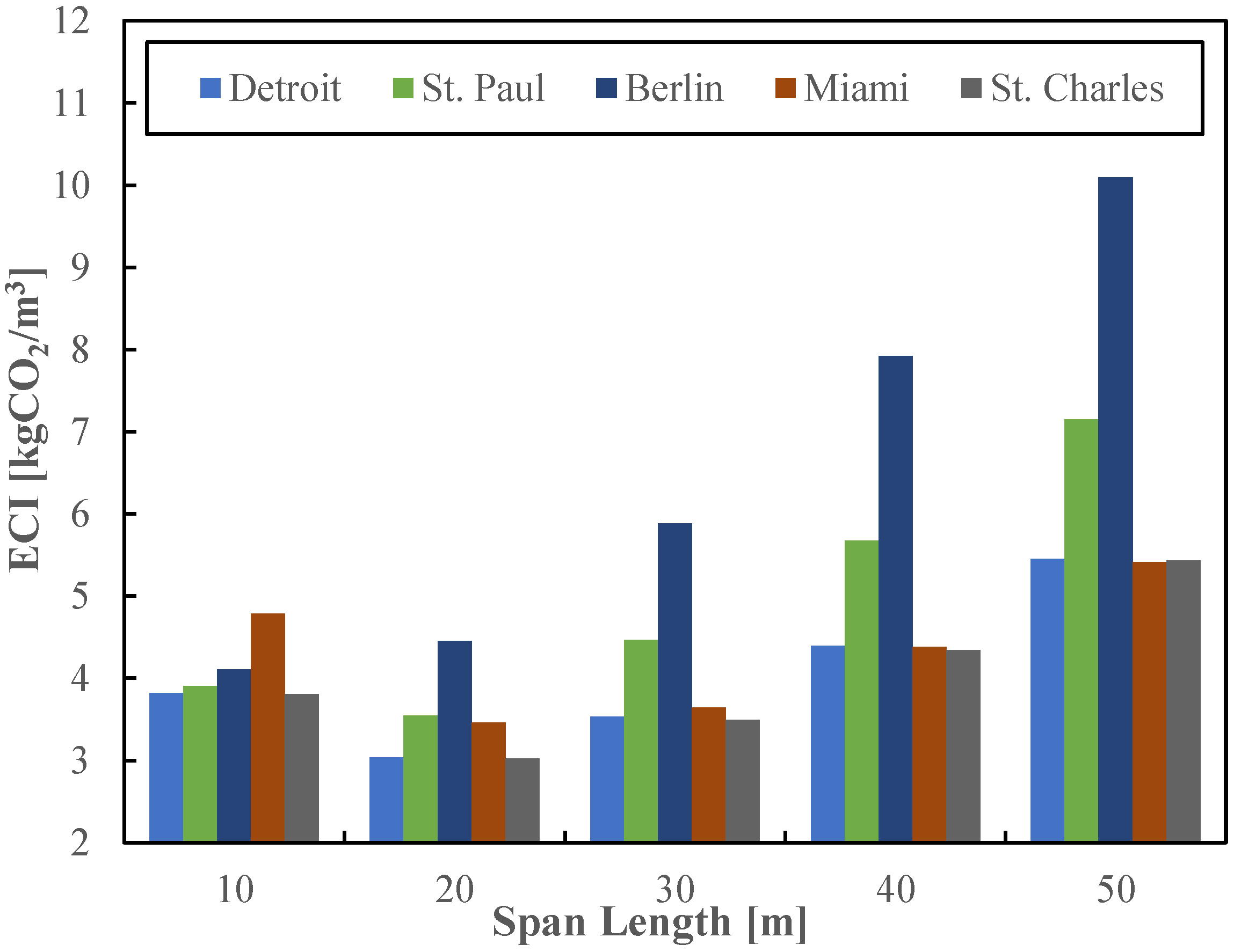
To investigate the effect of different loading conditions on the ECI of steel gable frames, Model 4 is considered as a case study in this section. The average ECI achieved by Model 4 for different span lengths and loading conditions is shown in Figure 8.
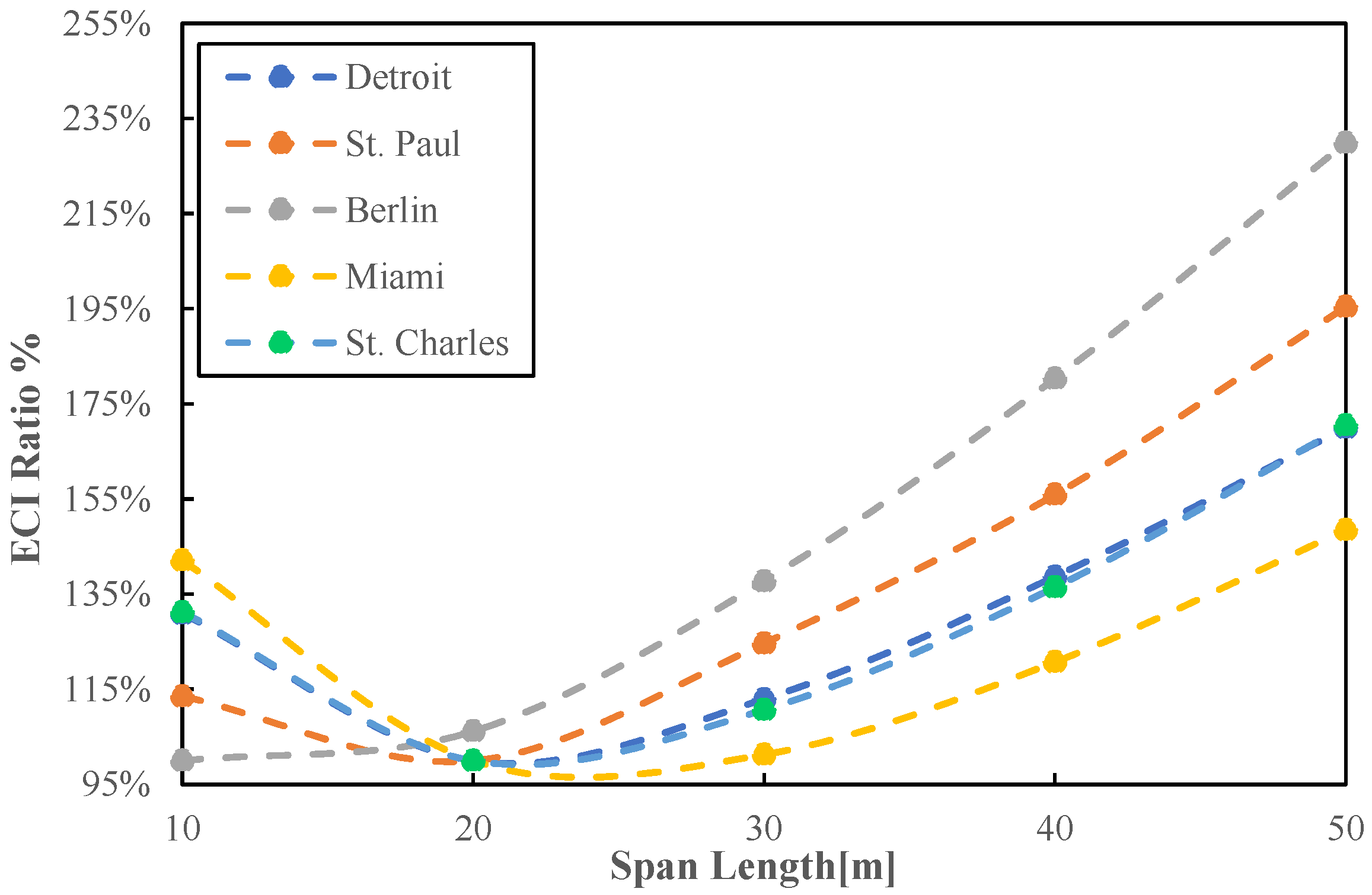
It can be observed that in the case of shorter span lengths, the loading condition causing the largest average ECI is the highest wind load (in Miami, FL), whereas the remaining loading conditions achieve almost the same ECI. However, as the span length increases, the ECI associated with almost all loading conditions (except for the highest snow load in Berlin, NH) decreases for the 20 m span length and then increases significantly for larger span lengths. The highest snow load (in Berlin, NH), however, causes the ECI of the steel frame to increase significantly as the span length increases to be the most critical loading condition for span lengths of 20 m and higher. This can be explained as follows. As span length increases, the high snow loads cause the straining actions to significantly increase, requiring larger steel sections with higher ECI. At the same time, the increase in the enclosed volume is not able to match the increase in the embodied carbon leading to an overall increase in the embodied carbon per unit of the enclosed volume by the steel frame. Furthermore, Figure 9 shows the ratio between the ECI for each span length and the least ECI across all spans for a specific loading condition. The same conclusions can be drawn as the highest wind load (in Miami, FL) is the most critical in the case of short spans (i.e., 10 m), while the highest snow load (in Berlin, NH) is the most critical for other span lengths. Another observation is that both Detroit and St. Charles achieved almost the same variation. This proves that the high seismic load is not effective in controlling the design of light, low-rise structures such as steel gable frames.
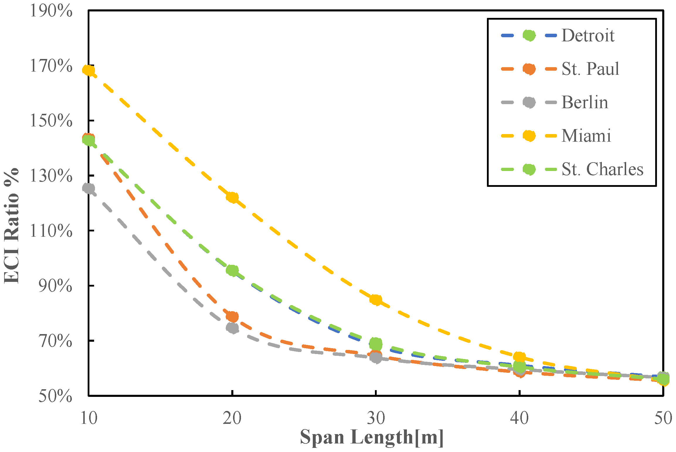
Finally, to investigate the difference of the ECI between the highest and lowest column heights (16 m and 6 m, respectively) for different span lengths, Figure 10 shows the ratio of the ECI of the 16 m column height case to that of the 6 m column height case for different span lengths and loading conditions for Model 4.
As Figure 10 shows, the loading condition causing the largest difference in the ECI for all span lengths is the case of the highest wind load (in Miami, FL), whereas the case of the highest vertical snow load (in Berlin, NH) results in the least difference between the column heights. Another observation is that both Detroit and St. Charles achieved almost the same variation which further proves the fact that the seismic load is not effective in controlling the design of steel gable frames. As the span length increases, the ratio between the ECI for the 16 m and 6 m cases decreases gradually for all loading conditions to reach a constant value at large span lengths (i.e., 50 m). The ECI for the 16 m column height frame is larger than that of the 6 m column height for short span lengths (i.e., 10 m). However, as the span length increases, the ECI ratio decreases at the highest rate in the case of the highest snow load (in Berlin, NH) and the lowest rate in the case of the highest wind load (in Miami, FL). The ECI for the 16 m column height case becomes less than that of the 6 m case for span lengths greater than 15 m and 26 m for the highest snow load and wind load, respectively.

7. Conclusions

In this study, various configurations of steel gable frames with both tapered and prismatic members are compared to determine the optimal configuration with the least embodied carbon, using a ‘cradle-to-cradle’ approach. Sizing, geometry, and topology optimization are performed to optimize the steel frames. The results of this study show the following:
  • For different frame configurations and loading conditions, contour plots showing the embodied carbon per unit of the enclosed volume by the steel frame (ECI) for different span lengths and column heights are prepared and can be used as design charts to determine the optimal span length and column height that achieve the least ECI.
  • In most cases, the minimum ECI can be achieved using frames with short-to-medium span lengths (i.e., around 20 m) and medium column heights (i.e., around 12 m).
  • For structural steel, Modules A1 and A3 have the largest contribution to the life-cycle positive embodied carbon of steel gable frames by about 75.3% and 16.5%, respectively. Whereas, Module D offsets the positive embodied carbon by about 30.6%.
  • The minimum ECI of a specific steel portal frame configuration can be reduced by increasing the number of member divisions, decision variables, and tapered segments.
  • Model 4 is able to achieve the highest ECI reduction relative to the control model by an average of 26.47%, followed by Models 2, 3, and 1 with ECI reduction of about 23.67%, 22.57%, and 14.34%, respectively.
  • For short span lengths, the difference between the different models is insignificant. However, as the span length increases, the average ECI reduction achieved by Models 2, 3, and 4 increases significantly, while that of Model 1 remains almost constant.
  • As the column height increases, the average ECI reduction achieved by Models 2, 3, and 4 slightly decreases, whereas that of Model 1 stays almost the same.

Author Contributions

Conceptualization, A.S. and A.E.; methodology, A.E. and A.A.F.; software, A.A.F.; validation, A.E. and A.A.F.; formal analysis, A.A.F.; investigation, A.A.F.; resources, A.E. and A.A.E.-S.; data curation, A.E.; writing—original draft preparation, A.A.F.; writing—review and editing, A.E., R.S. and A.A.E.-S.; visualization, A.A.F. and A.A.E.-S.; supervision, A.A.E.-S., A.S. and R.S.; project administration, A.S. and A.A.E.-S.; funding acquisition, A.E. and A.A.E.-S. All authors have read and agreed to the published version of the manuscript.

Funding

This research received no external funding.

Institutional Review Board Statement

Not applicable.

Informed Consent Statement

Not applicable.

Data Availability Statement

The data presented in this study are available on request from the corresponding author.

Conflicts of Interest

The authors declare no conflict of interest.

Appendix A. Contours of the Minimum ECI for Each Model

Figure A1. Contours of optimal frame ECI (kgCO 2 /m 3 ) for the control model: (a) Detroit, MI; (b) St. Paul, MN; (c) Berlin, NH; (d) Miami, FL; (e) St. Charles, KY.
Buildings 13 00739 g0a1
Figure A2. Contours of optimal frame ECI (kgCO 2 /m 3 ) for Model 1: (a) Detroit, MI; (b) St. Paul, MN; (c) Berlin, NH; (d) Miami, FL; (e) St. Charles, KY.
Buildings 13 00739 g0a2
Figure A3. Contours of optimal frame ECI (kgCO 2 /m 3 ) for Model 2: (a) Detroit, MI; (b) St. Paul, MN; (c) Berlin, NH; (d) Miami, FL; (e) St. Charles, KY.
Buildings 13 00739 g0a3
Figure A4. Contours of optimal frame ECI (kgCO 2 /m 3 ) for Model 3: (a) Detroit, MI; (b) St. Paul, MN; (c) Berlin, NH; (d) Miami, FL; (e) St. Charles, KY.
Buildings 13 00739 g0a4

References

  1. Zandalinas, S.I.; Fritschi, F.B.; Mittler, R. Global warming, climate change, and environmental pollution: Recipe for a multifactorial stress combination disaster. Trends Plant Sci. 2021, 26, 588–599. [Google Scholar] [CrossRef] [PubMed]
  2. Sala, O.E.; Stuart Chapin, F.; Armesto, J.J.; Berlow, E.; Bloomfield, J.; Dirzo, R.; Huber-Sanwald, E.; Huenneke, L.F.; Jackson, R.B.; Kinzig, A.; et al. Global biodiversity scenarios for the year 2100. Science 2000, 287, 1770–1774. [Google Scholar] [CrossRef] [PubMed]
  3. Mazdiyasni, O.; AghaKouchak, A. Substantial increase in concurrent droughts and heatwaves in the United States. Proc. Natl. Acad. Sci. USA 2015, 112, 11484–11489. [Google Scholar] [CrossRef] [PubMed] [Green Version]
  4. Lehmann, J.; Rillig, M. Distinguishing variability from uncertainty. Nat. Clim. Chang. 2014, 4, 153. [Google Scholar] [CrossRef]
  5. Bigot, S.; Buges, J.; Gilly, L.; Jacques, C.; Le Boulch, P.; Berger, M.; Delcros, P.; Domergue, J.B.; Koehl, A.; Ley-Ngardigal, B.; et al. Pivotal roles of environmental sensing and signaling mechanisms in plant responses to climate change. Glob. Chang. Biol. 2018, 24, 5573–5589. [Google Scholar] [CrossRef]
  6. Al-Ghussain, L. Global warming: Review on driving forces and mitigation. Environ. Prog. Sustain. Energy 2019, 38, 13–21. [Google Scholar] [CrossRef] [Green Version]
  7. Intergovernmental Panel on Climate Change. Global Warming of 1.5 °C; World Meteorological Organization: Geneva, Switzerland, 2018.
  8. Armstrong McKay, D.I.; Staal, A.; Abrams, J.F.; Winkelmann, R.; Sakschewski, B.; Loriani, S.; Fetzer, I.; Cornell, S.E.; Rockström, J.; Lenton, T.M. Exceeding 1.5 C global warming could trigger multiple climate tipping points. Science 2022, 377, eabn7950. [Google Scholar] [CrossRef]
  9. HM Government. The Carbon Plan: Delivering our low carbon future. In Proceedings of the Parliament Pursuant to Sections 12 and 14 of the Climate Change Act 2008, London, UK, 1 December 2011. [Google Scholar]
  10. United Nations. Net Zero Coalition. Available online: https://www.un.org/en/climatechange/net-zero-coalition (accessed on 10 December 2022).
  11. Vaughan, R. Government’s 2016 Zero-Carbon Homes Target ‘Too Unrealistic’. Available online: https://www.architectsjournal.co.uk/news (accessed on 14 December 2022).
  12. Ching, E.; Carstensen, J.V. Truss topology optimization of timber–steel structures for reduced embodied carbon design. Eng. Struct. 2022, 252, 113540. [Google Scholar] [CrossRef]
  13. Iddon, C.R.; Firth, S.K. Embodied and operational energy for new-build housing: A case study of construction methods in the UK. Energy Build. 2013, 67, 479–488. [Google Scholar] [CrossRef]
  14. Elavarasan, R.M.; Shafiullah, G.; Padmanaban, S.; Kumar, N.M.; Annam, A.; Vetrichelvan, A.M.; Mihet-Popa, L.; Holm-Nielsen, J.B. A comprehensive review on renewable energy development, challenges, and policies of leading Indian states with an international perspective. IEEE Access 2020, 8, 74432–74457. [Google Scholar] [CrossRef]
  15. Sartori, I.; Hestnes, A.G. Energy use in the life cycle of conventional and low-energy buildings: A review article. Energy Build. 2007, 39, 249–257. [Google Scholar] [CrossRef]
  16. Giordano, R.; Serra, V.; Tortalla, E.; Valentini, V.; Aghemo, C. Embodied energy and operational energy assessment in the framework of nearly zero energy building and building energy rating. Energy Procedia 2015, 78, 3204–3209. [Google Scholar] [CrossRef] [Green Version]
  17. Bahramian, M.; Yetilmezsoy, K. Life cycle assessment of the building industry: An overview of two decades of research (1995–2018). Energy Build. 2020, 219, 109917. [Google Scholar] [CrossRef]
  18. Nwodo, M.N.; Anumba, C.J. A review of life cycle assessment of buildings using a systematic approach. Build. Environ. 2019, 162, 106290. [Google Scholar] [CrossRef]
  19. Rezaei, F.; Bulle, C.; Lesage, P. Integrating building information modeling and life cycle assessment in the early and detailed building design stages. Build. Environ. 2019, 153, 158–167. [Google Scholar] [CrossRef] [Green Version]
  20. Hart, J.; D’Amico, B.; Pomponi, F. Whole-life embodied carbon in multistory buildings: Steel, concrete and timber structures. J. Ind. Ecol. 2021, 25, 403–418. [Google Scholar] [CrossRef]
  21. Pan, W.; Teng, Y. A systematic investigation into the methodological variables of embodied carbon assessment of buildings. Renew. Sustain. Energy Rev. 2021, 141, 110840. [Google Scholar] [CrossRef]
  22. Cang, Y.; Luo, Z.; Yang, L.; Han, B. A new method for calculating the embodied carbon emissions from buildings in schematic design: Taking “building element” as basic unit. Build. Environ. 2020, 185, 107306. [Google Scholar] [CrossRef]
  23. Malmqvist, T.; Nehasilova, M.; Moncaster, A.; Birgisdottir, H.; Rasmussen, F.N.; Wiberg, A.H.; Potting, J. Design and construction strategies for reducing embodied impacts from buildings–Case study analysis. Energy Build. 2018, 166, 35–47. [Google Scholar] [CrossRef] [Green Version]
  24. Pomponi, F.; Moncaster, A. Embodied carbon mitigation and reduction in the built environment—What does the evidence say? J. Environ. Manag. 2016, 181, 687–700. [Google Scholar] [CrossRef] [Green Version]
  25. D’Amico, B.; Pomponi, F. Accuracy and reliability: A computational tool to minimise steel mass and carbon emissions at early-stage structural design. Energy Build. 2018, 168, 236–250. [Google Scholar] [CrossRef] [Green Version]
  26. El-Sisi, A.E.D.A.; El-Husseiny, O.M.; Matar, E.B.; Sallam, H.E.D.M.; Salim, H.A. Field-testing and numerical simulation of vantage steel bridge. J. Civ. Struct. Health Monit. 2020, 10, 443–456. [Google Scholar] [CrossRef]
  27. El-Sisi, A.A.; Hassanin, A.I.; Shabaan, H.F.; Elsheikh, A.I. Effect of external post-tensioning on steel–concrete composite beams with partial connection. Eng. Struct. 2021, 247, 113130. [Google Scholar] [CrossRef]
  28. Allwood, J.M.; Cullen, J.M.; Carruth, M.A.; Cooper, D.R.; McBrien, M.; Milford, R.L.; Moynihan, M.C.; Patel, A.C. Sustainable Materials: With Both Eyes Open; UIT Cambridge Limited: Cambridge, UK, 2012; Volume 2012. [Google Scholar]
  29. Newman, A. Metal Building Systems Design and Specifications 2/E; Handbook; McGraw-Hill Education: New York, NY, USA, 2003. [Google Scholar]
  30. McKinstray, R.; Lim, J.B.; Tanyimboh, T.T.; Phan, D.T.; Sha, W. Optimal design of long-span steel portal frames using fabricated beams. J. Constr. Steel Res. 2015, 104, 104–114. [Google Scholar] [CrossRef] [Green Version]
  31. Firoz, S.; Kumar, S.C.; Rao, S.K. Design Concept of Pre Engineered Building. Int. J. Eng. Res. Appl. IJERA 2012, 2, 267–272. [Google Scholar]
  32. Davison, B.; Owens, G.W. Steel Designers’ Manual; John Wiley & Sons: Hoboken, NJ, USA, 2012. [Google Scholar]
  33. McKinstray, R.; Lim, J.B.P.; Tanyimboh, T.T.; Phan, D.T.; Sha, W. Comparison of optimal designs of steel portal frames including topological asymmetry considering rolled, fabricated and tapered sections. Eng. Struct. 2016, 111, 505–524. [Google Scholar] [CrossRef] [Green Version]
  34. Babaei, M.; Moharrami, H. Geometry and sizing optimization of steel gable frames with tapered members. Structures 2022, 42, 575–585. [Google Scholar] [CrossRef]
  35. Kaveh, A.; Hoseini Vaez, S.R.; Hosseini, P.; Bakhtyari, M. Optimal Design of Steel Curved Roof Frames by Enhanced Vibrating Particles System Algorithm. Period. Polytech. Civ. Eng. 2019, 63, 73–97. [Google Scholar] [CrossRef] [Green Version]
  36. Fu, J.Y.; Wu, J.R.; Dong, C.C.; Xu, A.; Pi, Y.L. Optimization design of large span portal-rigid steel frame with tapered sections under wind-induced drift constraint. Eng. Struct. 2019, 194, 396–405. [Google Scholar] [CrossRef]
  37. El-Sisi, A.; Alsharari, F.; Salim, H.; Elawadi, A.; Hassanin, A. Efficient beam element model for analysis of composite beam with partial shear connectivity. Compos. Struct. 2023, 303, 116262. [Google Scholar] [CrossRef]
  38. Kaveh, A.; Ghafari, M.H. Geometry and Sizing Optimization of Steel Pitched Roof Frames with Tapered Members Using Nine Metaheuristics. Iran. J. Sci. Technol. Trans. Civ. Eng. 2018, 43, 1–8. [Google Scholar] [CrossRef]
  39. Saka, M. Optimum design of steel frames with tapered members. Comput. Struct. 1997, 63, 797–811. [Google Scholar] [CrossRef]
  40. Saka, M. Optimum design of pitched roof steel frames with haunched rafters by genetic algorithm. Comput. Struct. 2003, 81, 1967–1978. [Google Scholar] [CrossRef]
  41. Kaveh, A.; Biabani Hamedani, K.; Milad Hosseini, S.; Bakhshpoori, T. Optimal design of planar steel frame structures utilizing meta-heuristic optimization algorithms. Structures 2020, 25, 335–346. [Google Scholar] [CrossRef]
  42. Chen, Y.; Hu, K. Optimal design of steel portal frames based on genetic algorithms. Front. Archit. Civ. Eng. China 2008, 2, 318–322. [Google Scholar] [CrossRef]
  43. McKinstray, R.; Lim, J.B.; Tanyimboh, T.T.; Phan, D.T.; Sha, W.; Brownlee, A.E. Topographical optimisation of single-storey non-domestic steel framed buildings using photovoltaic panels for net-zero carbon impact. Build. Environ. 2015, 86, 120–131. [Google Scholar] [CrossRef] [Green Version]
  44. De Wolf, C.; Yang, F.; Cox, D.; Charlson, A.; Hattan, A.S.; Ochsendorf, J. Material quantities and embodied carbon dioxide in structures. In Proceedings of the Institution of Civil Engineers—Engineering Sustainability; Thomas Telford Ltd.: London, UK, 2015. [Google Scholar] [CrossRef]
  45. Drewniok, M.P.; Campbell, J.; Orr, J. The Lightest Beam Method–A methodology to find ultimate steel savings and reduce embodied carbon in steel framed buildings. In Proceedings of the Structures; Elsevier: Amsterdam, The Netherlands, 2020; Volume 27, pp. 687–701. [Google Scholar]
  46. ANSI/AISC 360-16; Specification for Structural Steel Buildings. AISC: Chicago, IL, USA, 2016.
  47. ANSI/AISC 341-16; Seismic Provisions for Structural Steel Buildings. American Institute of Steel Construction: Chicago, IL, USA, 2016.
  48. ASCE/SEI 7-16; Minimum Design Loads and Associated Criteria for Buildings and Other Structures. American Society of Civil Engineers: Reston, VA, USA, 2017.
  49. White, D.W.; Jeong, W.Y.; Slein, R. Design Guide 25: Frame Design Using Nonprismatic Members, 2nd ed.; AISC: Chicago, IL, USA, 2021. [Google Scholar]
  50. Liu, J.; Teo, K.L.; Wang, X.; Wu, C. An exact penalty function-based differential search algorithm for constrained global optimization. Soft Comput. 2015, 20, 1305–1313. [Google Scholar] [CrossRef]
  51. The Mathworks, Inc. MATLAB Version 8.5.0.197613 (R2015a); The Mathworks, Inc.: Natick, MA, USA, 2015. [Google Scholar]
  52. Cook, R.D.; Malkus, D.S.; Plesha, M.E.; Witt, R.J. Concepts and Applications of Finite Element Analysis, 4th ed.; Wiley: Hoboken, NJ, USA, 2001. [Google Scholar]
  53. Cowper, G.R. The Shear Coefficient in Timoshenko’s Beam Theory. J. Appl. Mech. 1966, 33, 335–340. [Google Scholar] [CrossRef]
  54. Talatahari, S.; Azizi, M.; Tolouei, M.; Talatahari, B.; Sareh, P. Crystal Structure Algorithm (CryStAl): A Metaheuristic Optimization Method. IEEE Access 2021, 9, 71244–71261. [Google Scholar] [CrossRef]
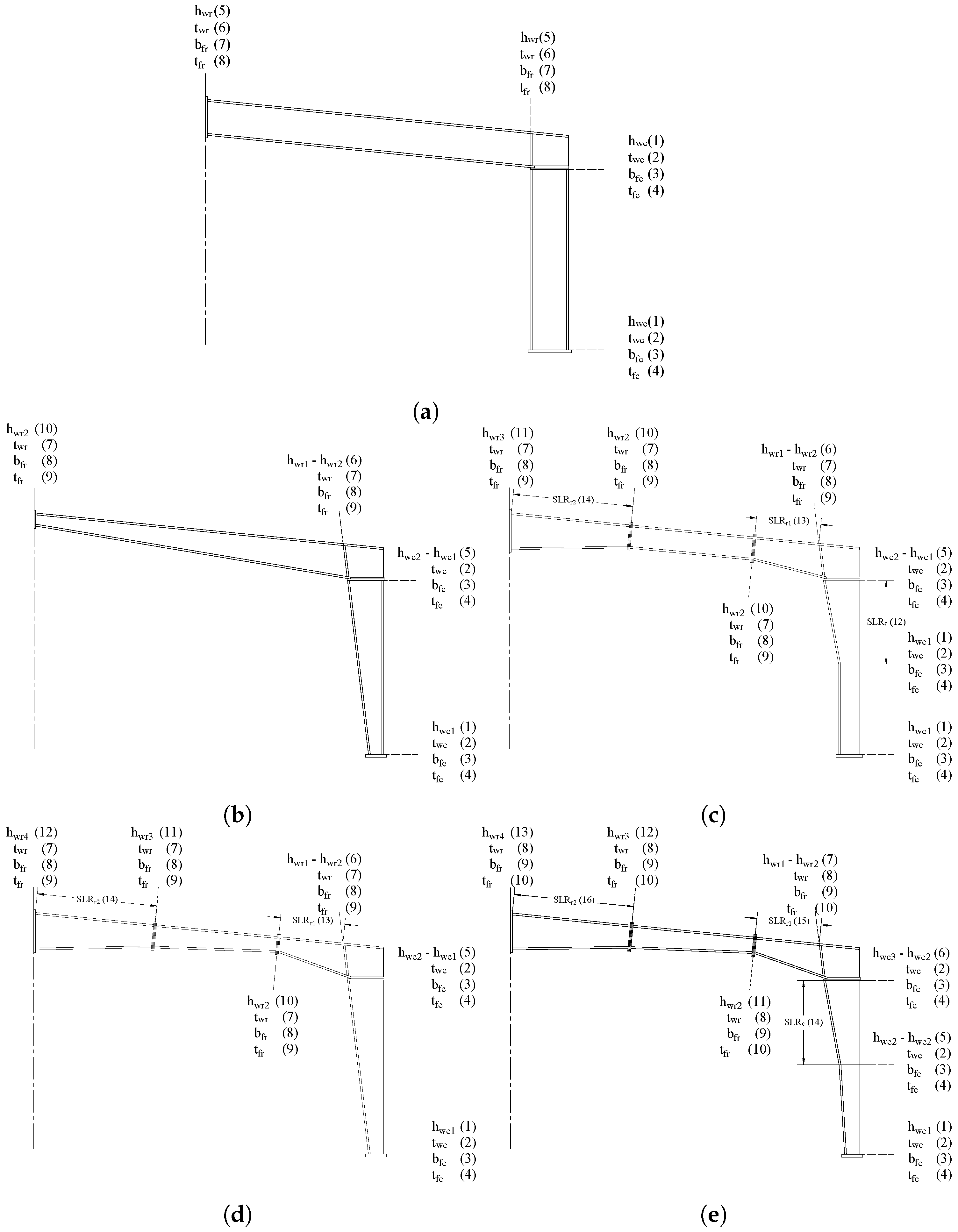
Figure 1. Utilized gable frame configurations and design variables: (a) control model; (b) Model 1; (c) Model 2; (d) Model 3; (e) Model 4.
Buildings 13 00739 g001
Figure 2. Contours of optimal frame ECI (kgCO 2 /m 3 ) for Model 4: (a) Detroit, MI; (b) St. Paul, MN; (c) Berlin, NH; (d) Miami, FL; (e) St. Charles, KY.
Buildings 13 00739 g002
Figure 3. Average ECI variation with span length for different models.
Buildings 13 00739 g003
Figure 4. Average ECI variation with column height for different models.
Buildings 13 00739 g004
Figure 5. Average contribution of different modules in the ECI for each model.
Buildings 13 00739 g005
Figure 6. Average ECI reduction variation with span length for different models.
Buildings 13 00739 g006
Figure 7. Average ECI reduction variation with column height for different models.
Buildings 13 00739 g007
Figure 8. Average ECI achieved by Model 4 for different span lengths and loading conditions.
Buildings 13 00739 g008
Figure 9. Average ECI ratio variation with span length for different load conditions.
Buildings 13 00739 g009
Figure 10. Varitation of the ECI ratio between the frames with 16 m and 6 m column heights with span length.
Buildings 13 00739 g010
Table 1. Design variables discrete values.
VariableUnitDiscrete ValuesNumber of Discrete Values
h w c mm250:+10:1500126
h w c j h w c i mm0:+10:1250126
t w c mm6:+2:124
b f c mm130:+10:30018
t f c mm6:+2:4018
h w r mm250:+10:1500126
h w r j h w r i mm0:+10:1250126
t w r mm6:+2:124
b f r mm130:+10:30018
t f r mm6:+2:4018
S L R c %10%:+5%:90%17
S L R r 1 %10%:+5%:80%15
S L R r 2 %10%:+5%:80%15
Table 2. Strength constraints.
Straining ActionLimit
Combined compression and bending P u 2 P c + M u x M c x + M u y M c y 1 , P u P c < 0.2 P u P c + 8 9 M u x M c x + M u y M c y 1 , P u P c 0.2
Combined tension and bending P u P c + M u x M c x + M u y M c y 1
Shear force V u V c 1
Table 3. Serviceability constraints.
Load CaseApex Vertical DisplacementEave Horizontal Displacement
Total LoadsLive LoadTotal LoadsSeismic Load
Limit δ v L / 240 δ v L / 360 δ h h / 200 δ M 0.02 h
Table 4. Snow load parameters.
Parameter C e I s C t ExposureRisk CategorySurface Roughness
Value1.01.01.0Partially exposedIIB
Table 5. Wind load parameters.
Parameter K e K zt K d Surface RoughnessEnclosure ClassBuilding HeightExposure Category
Value1.01.00.85BEnclosedLow-riseB
Table 6. Seismic load parameters.
Parameter I e R C d Risk CategoryStructural SystemSite Class
Value1.03.53.5IIOrdinary moment frameD
Table 7. Loading parameters of different frame locations.
LocationSeismic Parameters
P g
[N/m2]
V
[m/s]
T L
[s]
S 1
-
S s
-
F a
-
F v
-
St. Charles, KY, USA71847120.1920.4791.4172.216
Miami, FL, USA07680.020.041.62.4
Berlin, NH, USA43104860.0750.2581.5942.4
St. Paul, MN, USA239549120.030.0471.62.4
Detroit, MI, USA96048120.0460.1031.62.4
Table 8. A sample of the optimal designs of different models.
GWP [kgCO2]ColumnRafter SLR c
%
SLR r 1
%
SLR r 2
%
h w bot .
[mm]
h w mid .
[mm]
h w top
[mm]
t w
[mm]
b f
[mm]
t f
[mm]
h w edge
[mm]
h w int . 1
[mm]
h w int . 2
[mm]
h w mid .
[mm]
t w
[mm]
b f
[mm]
t f
[mm]
Control Model2952480-48062208650--65061506---
Model 12591250-87061906810--25061606---
Model 22192280280950614068202602605906130675%30%60%
Model 32271250-8906170682032025050061306-30%55%
Model 42181250680780613067602602606506130630%30%55%
Table 9. Average ECI reduction of Models 1, 2, 3, and 4 compared to the control model.
Model 1Model 2Model 3Model 4
ECI Reduction %14.34%23.67%22.57%26.47%
Disclaimer/Publisher’s Note: The statements, opinions and data contained in all publications are solely those of the individual author(s) and contributor(s) and not of MDPI and/or the editor(s). MDPI and/or the editor(s) disclaim responsibility for any injury to people or property resulting from any ideas, methods, instructions or products referred to in the content.