Abstract
Most regional seismic damage assessment (RSDA) methods are based on the rigid-base assumption to ensure evaluating efficiency, while these practices introduce factual errors due to neglecting the soil–structure interaction (SSI). Predicting the influence of the SSI on seismic responses of regionwide structure portfolios remains a challenging undertaking, as it requires developing numerous high-fidelity, integrated models to capture the dynamic interplay and uncertainties in structures, foundations, and supporting soils. This study develops a one-dimensional convolutional neural network (1D-CNN) model to efficiently predict to what degree considering the SSI would change the inter-story drifts and base shear forces of RC frame buildings. An experimentally validated finite element model is developed to simulate the nonlinear seismic behavior of the building-foundation–soil system. Subsequently, a database comprising input data (i.e., structural and soil parameters, ground motions) and output predictors (i.e., changes in story drift and base shear) is constructed by simulating 1380 pairs of fixed-base versus soil-supported structures under earthquake loading. This large-scale dataset is used to train, test, and identify the optimal hyperparameters for the 1D-CNN model to quantify the demand differences in inter-story drifts and base shears due to the SSI. Results indicate the 1D-CNN model has a superior performance, and the absolute prediction errors of the SSI influence coefficients for the maximum base shear and inter-story drift are within 9.3% and 11.7% for 80% of cases in the testing set. The deep learning model can be conveniently applied to enhance the accuracy of the RSDA of RC buildings by updating their seismic responses where no SSI is considered.
1. Introduction
Rapid regional seismic damage assessment (RSDA) of civil engineering structures provides situational awareness toward efficient post-earthquake rescue, repair, and reconstruction, which can reduce casualties, injuries, and economic losses. High-fidelity RSDA can be achieved through nonlinear time-history analysis (NLTHA) to reliably predict the seismic responses of structural systems. To save computational cost, previous studies mainly relied on the rigid-base assumption to conduct NLTHAs for the RSDA of building structures [1,2]. The rigid-base assumption neglects the dynamic interaction between the soil and structure; the same assumption has also been commonly considered in the seismic design and retrofit of new and existing buildings [3,4,5]. However, neglecting the soil–structure interaction (SSI) effect may introduce a significant error, particularly for tall buildings built on soft soils [6,7].
The SSI effect remains a complex and challenging research topic because it couples many uncertain parameters in the soil, foundation, superstructure, and seismic records. Early studies [8,9] generally agreed that considering the SSI is beneficial to the seismic performance of building structures as the SSI can lengthen the natural period of the system [10] and provide additional damping. However, recent studies have found that considering the SSI could also significantly increase the seismic demands of building structures in certain cases due to (1) the rocking of the foundation [11], (2) earthquake-induced soil liquefaction [12], and (3) the resonance effect between the soil and superstructure [13], etc. Two examples are further discussed here. First, Tomeo et al. [14] used a refined finite element model to investigate the SSI effect on the seismic responses of reinforced concrete (RC) frames with different subsoil properties and seismic design levels. They found that the SSI could reduce the structure’s maximum story drift and base shear up to 50% and 20%, respectively. In contrast, Hokmabadi et al. [15] investigated the influence of soil–pile–structure interaction on the seismic responses of mid-rise buildings by a series of shaking table tests, finding that the SSI increases the lateral deflections and inter-story drifts of soil-supported structures in comparison with the fixed-base structures and the increase is up to 34%. In addition, they pointed out that ignoring the SSI effect may lead to erroneous evaluations of structural seismic demands.
In view of the considerable impact of the SSI on structural seismic responses, some approaches to consider the SSI have been proposed in recent years. Lu et al. [16] developed a numerical coupling scheme to conduct an RSDA of building–soil systems, where the spectral element program SPEED [17] was employed to simulate wave propagation in underlying soil layers. Lu et al. [18] and Zhang et al. [19] also developed a three-dimensional lumped parameter model (LPM) to account for the SSI effect in the seismic response prediction of Wangjiang Campus buildings in Sichuan University, China. Forcellini [20] proposed a framework to assess the SSI effects with an equivalent fixed-based model that considers the SSI effects by applying the period of elongation and the damping increase. These studies have considered the SSI effects to some extent. However, the neglect of the soil embedment of structural foundations in these studies may introduce errors. For example, El Hoseny et al. [21] investigated the SSI effects on the seismic responses of tall buildings with variable embedded depths, pointing out that the embedded depth can significantly affect the structural seismic response.
Moreover, the recent advances in data science have provided many opportunities to leverage statistical and machine learning to solve challenging problems in structural and earthquake engineering [22,23]. For example, Won et al. [24] developed an artificial neural network to determine the seismic damage levels of regional buildings. Duarte et al. [25] proposed a convolutional neural network (CNN) to delineate damaged regions and assess building damage by remote sensing. Xu et al. [26] developed a long short-term memory (LSTM) neural network to achieve a real-time RSDA. Likewise, rapid RSDA was proposed by Lu et al. [27] through a CNN model that analyzes the time-frequency features of ground motions. These studies have made valuable attempts to explore the promise of using machine learning to enhance the accuracy and efficiency of RSDAs. However, no relevant research has been conducted to predict the influence of the SSI on the seismic responses of RC frame buildings.
To efficiently and accurately predict what degree considering the SSI would change the inter-story drifts and base shear forces of RC frame buildings, an experimentally validated finite element model is established to obtain the SSI effect on pile-supported RC frame structures. Subsequently, a dataset of 1380 input (i.e., structural and soil parameters, ground motions) and output parameters (i.e., changes in story drift and base shear) is established through the finite element analyses of numerous fixed-base versus soil-supported structures under earthquake loading. A one-dimensional convolutional neural network (1D-CNN) is then developed to quantify the response differences in the inter-story drift and base shear due to the SSI (i.e., between fixed-base and soil-supported structures). Furthermore, a parametric study is conducted to pinpoint the optimal set of hyperparameters that bear a proper balance between the model accuracy and efficiency. Results indicate that the developed 1D-CNN model can well predict the influence of the SSI on the seismic responses of RC frame buildings. The absolute prediction errors of the SSI influence coefficients for the maximum base shear and inter-story drift are within 9.3% and 11.7% for 80% of cases in the testing set.
2. Numerical Model to Account for SSI Effects
2.1. Numerical Model
A two-dimensional SSI model is established based on the platform OpenSees, as shown in Figure 1. The soil is simulated by assigning the constitutive model PressureIndependMultiYield (PIMY) [28] to the four-node quad elements. The PIMY model is an elastic–plastic material, which can reflect the nonlinear behavior of soil under fast loading conditions. The displacement-based beam–column elements are employed to simulate the beam, column, pile, and pile cap, where the constitutive models of the concrete and reinforcement are Concrete02 [29] and Steel02 [30], respectively. The soil nodes and pile nodes at the same positions are fully coupled according to Mercado et al. (2021) [31]. The connection between the pile cap and soil is shown in the blue circle in Figure 1, where the translational degrees of freedom (DOFs) of the pile cap node and soil node are tied in the horizontal direction; the vertical translation DOFs of the pile cap node and soil node are connected by using the Zerolength element, and the Elastic-No Tension (ENT) material is assigned to the Zerolength element to simulate the opening and closing between the pile cap and soil. The lateral boundaries of the soil are set as shear boundaries [32], where the horizontal translation DOFs of the nodes at the same height on the two lateral soil boundaries are tied to simulate the shear deformation of the soil under earthquake loadings. The bottom of the soil is considered bedrock, and seismic excitations are imposed by inputting the bedrock acceleration time histories to the bottom nodes of the soil.
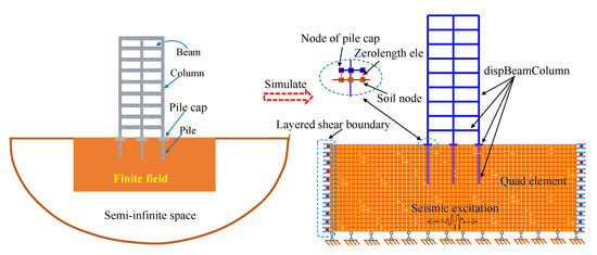
Figure 1.
Schematic diagram for illustrating soil–structure interaction model.
2.2. Validation of the Numerical Model
Results from two shaking table tests (i.e., one is a free field test, and the other is an SSI test [33]) are utilized to validate the effectiveness of the numerical model. For the SSI test, the volumetric dimension (length × width × height), density, and shear wave velocity of the hypothetical prototype soil are 58 m × 40 m × 25 m, 1.65 ton/m3, and 120 m/s, respectively; the height and plane dimension of the hypothetical prototype single degree of freedom (SDOF) structure are 12.1 m and 6.0 m × 6.0 m. According to the plane dimensions of the prototype soil and superstructure, and the size and performance of the shaking table, the similarity ratio of the length, density, and elastic modulus are set as 1:20, 1:1.5, and 1:6, respectively. As such, the volumetric dimension, density, and shear wave velocity of the tested soil are 2.9 m × 2.0 m × 1.25 m, 1.1 ton/m3, and 60 m/s, respectively. As shown in Figure 2, the laminated shear soil box is employed to ensure that the soil deforms in shear [34,35]; the soil is selected as the sawdust soil, and an SDOF structure is chosen to be supported by a pile foundation. The pile length, pile diameter, structure height, and fixed-base structural period of the tested SDOF structure (Figure 2c) are 0.4 m, 0.04 m, 0.605 m, and 0.05 s, respectively. Acceleration sensors are placed at the center of the surface soil and the top of the SDOF structure in the free field and SSI tests, respectively. The time-history accelerations for the free field test and SSI test are shown in Figure 3a,b, respectively.

Figure 2.
Field test photos and finite element models.
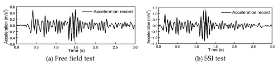
Figure 3.
Seismic records used in the tests.
The finite element models developed for the shaking table tests are illustrated in Figure 2b,d, where the mesh size of the soil is set as 0.05 m to ensure the influence of the mesh size is negligible. The reference low-strain shear modulus (Gr), reference bulk modulus (Br), cohesion (c), and peak shear strain (γmax) of the soil are, respectively, set as 3600 kPa, 18,000 kPa, 14 kPa, and 0.1, and the other parameters are set as default values. By inputting the acceleration time histories at the bottom of the soil, time-history analyses are conducted on the finite element models to obtain the acceleration responses at the center of the surface soil for the free field test, and the acceleration at the top of the SDOF structure for the SSI test. As shown in Figure 4a,b, the numerical outcomes and test results are in good agreement, indicating that the numerical model of the soil–SDOF structure system is reliable. The only difference between the soil–SDOF structure system and the soil–frame structure system is the superstructure. The modeling method of the frame structure adopted in this paper has been widely used and validated [3,31]; thus, the presented numerical model for the soil–frame structure system is reliable. Noting that simplifying the real frame structure into an idealized SDOF structure will introduce errors [36], the subsequent studies adopt soil–frame structure models.

Figure 4.
Comparisons between simulation outcomes and experiment results.
3. Database Construction
Two factors, esd and ebs, are defined in Equations (1) and (2) to quantify the influences of the SSI effect on two significant seismic demand parameters, namely the maximum inter-story drift and maximum base shear. In these two equations, SSSI and Sfb denote the maximum story drifts of the structure with and without considering the SSI (i.e., a fixed-base structure), whereas BSSI and Bfb denote the maximum base shear forces of the structure with and without considering the SSI. In particular, Sfb and Bfb are obtained by imposing the ground motion recorded at the soil surface to the base of the fixed-base structure, while SSSI and BSSI are obtained by imposing the bedrock motion to the soil bottom. To ensure the seismic excitations of the structures with and without considering the SSI are consistent, the bedrock motions corresponding to the ground motion recorded at the soil surface are obtained by performing deconvolutional analyses using SHAKE [37] and used for the soil–structure system.
Previous studies [38,39] revealed that the SSI effects are significantly influenced by the seismic record, soil shear wave velocity, building’s natural frequency, bay number, and pile diameter. Moreover, the maximum influence of the pile length on the SSI effects can still be up to about 10% in some cases [40]. As such, 1380 pairs of finite element models for fixed-base versus soil-supported RC frames are developed to investigate the SSI effects. To adequately capture the influences and uncertainties of earthquake loading, 270 seismic records with different spectral characteristics are selected from the PEER Ground Motion Database [41], and they are randomly scaled to have peak ground accelerations (PGAs) stay in the range of 0 to 4.0 m/s2. In particular, the seismic record for each fixed-base structure is randomly selected from the 270 seismic records, and the bedrock motion (obtained using SHAKE) corresponding to this seismic record is used for the soil-supported RC frame corresponding to this fixed-base structure. Figure 5 presents the finite element models of the fixed-base versus the soil-supported RC frames, where the story height and bay length are 3.3 m and 6.0 m, the longitudinal reinforcement ratio of each side for column is 0.33%, and the longitudinal reinforcement ratio of the beam top, beam bottom, and pile are 0.6%, 0.4%, and 0.8%, respectively. The cross-section dimensions of the beams and columns affect the SSI effect mainly by changing the structural frequency. As such, two series of RC frames (F1-1 to F15-1 and F1-2 to F15-2) with different cross-section dimensions of beams and columns are designed to fully consider the variation in the structural frequency, as shown in Table 1, where C45 concrete with the nominal cubic compressive strength of 45 MPa and HRB335 steel with the nominal yield strength of 335 MPa are used [42]. In addition, the height of the supporting soils is 20 m [43], and the soil lengths are 60 m, 60 m, 60 m, 78 m, and 98 m when the bay number is increased from one to five, ensuring that the influence of the artificial soil boundary is negligible. The values of the other parameters for each pair of fixed-base versus soil-supported structures are randomly selected from Table 2.
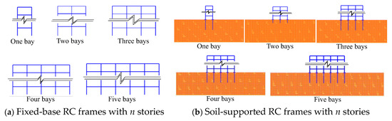
Figure 5.
Finite element models for RC frames with and without considering SSI.

Table 1.
Detailed information of RC frames with different stories.
Table 2.
Value ranges of parameters for fixed-base versus soil-supported structures.
The Fourier spectra can well reflect the frequency characteristics and peak acceleration of the seismic record, and the main frequency components of most seismic records recorded at the soil surface are within 16 Hz. As such, 328 Fourier amplitudes with a frequency interval of 0.049 Hz are used to represent the seismic record. To this end, a dataset consisting of 1380 groups of building-motion couples is established, where 270 ground motions are randomly coupled with 1380 pairs of fixed-base versus soil-supported RC frames designed with different structure, pile, and soil parameters. A schematic data inventory information is shown in Figure 6, where the input parameters include 328 Fourier amplitudes of the seismic record and 6 soil–structure parameters, namely the soil shear wave velocity, building’s natural frequency, story number, bay number, and pile length and diameter, and ebs and esd are the two predictors.
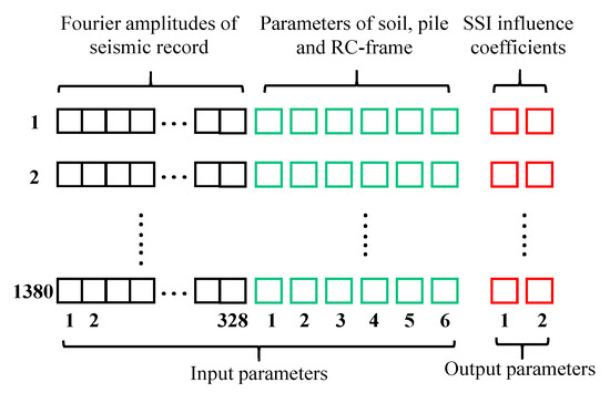
Figure 6.
Structure diagram of the dataset.
4. 1D-CNN to Quantify the SSI Effect
4.1. Development of the 1D-CNN Model
Convolutional neural network (CNN) employs a convolutional computation algorithm to extract the main features of input data. The mathematical expression of the algorithm is presented in Equation (3), where M denotes the number of output feature maps for the (l−1)th layer; denotes the ith output feature map of the (l−1)th layer; denotes the jth output feature map of the lth layer; denotes the jth convolution kernel (filter) of the lth layer; denotes the jth bias of the lth layer; “*” denotes the convolutional computation; and f (·) is the activation function.
The input of the one-dimensional convolutional neural network (1D-CNN) is one-dimensional vectors instead of two-dimensional pictures. Therefore, the convolution operation cost of the 1D-CNN is significantly reduced as compared with a typical CNN. To speed up the convolution operation, a 1D-CNN, as shown in Figure 7, is established to predict ebs and esd using the dataset obtained through the nonlinear time-history analyses. The 1D-CNN model is designed with an input layer, two convolutional pooling layers named Conv1 and Conv2, a fully connected layer, and an output layer. In particular, 1380 groups of input and output parameters are randomly divided into 1130 groups for training and 250 groups for testing. To reduce the magnitude difference in the data, the mapminmax function shown in Equation (4) is utilized to normalize the original input data before feeding them into the input layer. The 1D-CNN is designed with a relatively simple architecture consisting of two convolution layers to avoid potential overfitting. The pooling size and stride are set as 1 in each pooling layer to prevent information loss when describing the soil–structure system. The widely used function, rectified linear unit (Relu), as shown in Equation (5), is adopted as the activation function. The dropout function is applied after the convolution layers to alleviate overfitting. The adaptive moment estimation (Adam) [44] optimizer is adopted to train the CNN model, and the initial learning rate is determined as 0.001. In addition, the mini-batch gradient descent method is used to improve the generalization ability of the 1D-CNN model.
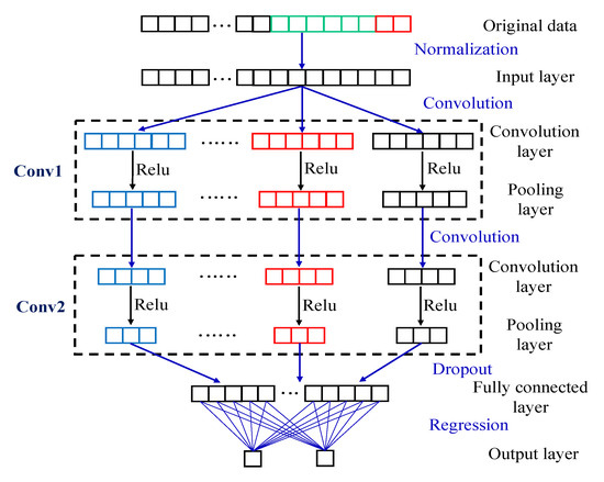
Figure 7.
Structure diagram of the 1D-CNN model.
4.2. Sensitivity Analyses of Hyperparameters for Training the 1D-CNN Model
The selection of hyperparameters is further investigated through sensitivity analyses to improve the accuracy and efficiency of the 1D-CNN model. These include architecture parameters, such as the strides, sizes, and the number of filters, and training parameters, such as the batch size and epochs. In addition, the influence of the size of the training set on the performance of the 1D-CNN model is also explored. Using the coefficient of determinations (R2), mean absolute error (Eabs), and training time as the evaluation metrics, sensitivity analyses are conducted to determine each parameter to have a proper balance between the accuracy and efficiency. Table 3 lists the results for selecting the number of filter strides using the benchmark 1D-CNN model designed with (3, 3) and (32, 64) as the sizes and number of filters for the two convolution layers, as well as 128 and 500 as the batch size and epochs. As shown in Table 3, 1 stride for both convolution layers will provide the best performance in accuracy (largest R2 and smallest Eabs) yet requires a reasonable amount of training time. In all the following tables, the cases with best performances have been highlighted by bold.
Table 3.
Influence of filter stride on the performance of the 1D-CNN model.
Six 1D-CNN models are developed to have (1, 1), (3, 3), 128, and 500 as the filter stride, filter size, batch size, and epochs; these models are designed to have different filter numbers to investigate their influences on the model performance. As shown in Table 4, training the 1D-CNN model requires more time when the filter number is increased. In addition, the model performance does not always increase with the increase in the filter numbers, and the best predicting accuracy (Eabs for ebs and esd in the testing set is smallest) is observed when the filter numbers of the first and second convolution layers are 16 and 64, respectively.
Table 4.
Influence of the number of filters on the performance of the 1D-CNN model.
Five different 1D-CNN models are developed to investigate the influence of the filter size, where other hyperparameters such as the filter stride, filter number, batch size, and epochs are determined as (1, 1), (16, 64), 128, and 500, respectively. As shown in Table 5, the filter size does not greatly affect the accuracy and training time of the model. In particular, R2 and Eabs for the training set indicate the best model performance when the filter sizes are 3 and 3 for the first and second convolution layers, respectively.
Table 5.
Influence of the sizes of filters on the performance of the 1D-CNN model.
Four 1D-CNN models are established to investigate the influence of the size of the training set on the performance of the 1D-CNN model, where the filter stride, filter size, filter number, batch size, and maximum epochs number are (1, 1), (3, 3), (16, 64), 128, and 500, respectively. Table 6 shows that both the model accuracy and training time increase when the size of the training set is increased from 750 to 1130.
Table 6.
Influence of the size of training set on the performance of the 1D-CNN model.
The maximum number of epochs would also affect the performance of the 1D-CNN model. Using five 1D-CNN models that have the filter stride, filter size, filter number, and batch size chosen as (1, 1), (3, 3), (16, 64), and 128, the results regarding the influences of the epoch number are presented in Table 7. In general, R2 and the training time will increase, while Eabs will decrease when the maximum number of epochs is increased from 250 to 1000.
Table 7.
Influence of the number of maximum epochs on the performance of the 1D-CNN model.
Likewise, Table 8 explores the influence of the batch size on the performance of the 1D-CNN model. Other hyperparameters of the model are determined through the sensitivity analyses discussed above. Namely, the filter stride, filter size, filter number, and maximum epochs number are (1, 1), (3, 3), (16, 64), and 1000, respectively. As listed in the Table, the model performance does not always decrease when the batch size is increased from 16 to 128. The 1D-CNN model has the best performance when the batch size is 32.
Table 8.
Influence of batch size on the performance of the 1D-CNN model.
4.3. Performance of the 1D-CNN Model
According to sensitive analyses, the strides, sizes, and numbers of filters for the 1D-CNN model are finally selected as (1, 1), (3, 3), and (16, 64), respectively, whereas 32 batches and 1000 epochs are considered for the model. As a result, the training time of the model turns out to be 1076 s. The comparisons between the predicted values and true values for esd and ebs of the training set are shown in Figure 8a,b, and those for ebs and esd of the testing set are shown in Figure 8c,d, respectively. It is found that the predicted values and true values of most samples in both the training set and testing set are close.
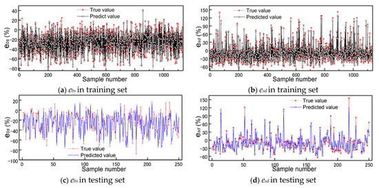
Figure 8.
Comparisons between predicted values and true values of SSI influence coefficients.
To illustrate the performance of the 1D-CNN model in detail, Figure 9 presents the predicted versus true values of ebs and esd together with the associated R2 values, and Figure 10 shows the cumulative distribution function (CDF) curves of the absolute errors between the predictions and ground truths. Figure 9 shows that R2 for ebs and esd in the testing sets are up to 0.928 and 0.941, indicating highly correlated predictions against the true values. In particular, R2 for the testing set is close to those for the training set, thereby no overfitting being observed. In addition, it can also be found that the values of ebs range from −80% to 40% and the values of esd range from −70% to 150%. Figure 10 shows that the absolute errors of ebs and esd for the 80-percentile CDFs are within 6.4% and 8.7% for the training set and are within 9.3% and 11.9% for the testing set. The above observations indicate that the 1D-CNN model can well predict the influence of the SSI on the seismic responses of RC frame buildings.
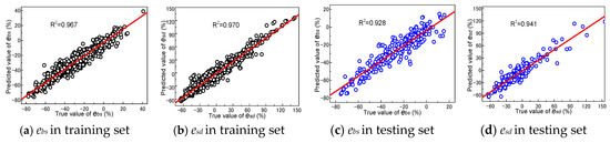
Figure 9.
Relationships between predicted values and true values.

Figure 10.
CDF curves of absolute error between predicted values and true values of SSI influence coefficients.
5. Conclusions
This study develops a 1D-CNN model to quantify the influence of the SSI on the seismic responses of regional RC frame buildings. Focusing on predicting what degree considering the SSI would change the structural inter-story drifts and base shears, an extensive set of finite element analyses are conducted to provide datasets for training and testing the CNN model and identifying its optimal hyperparameters. The following conclusions can be drawn from the current study.
(1) Compared with the fixed-base structure, the influence of the SSI on the structural maximum base shear ranges from −80% to 40% and that on the structural maximum story drift it ranges from −70% to 150%.
(2) The developed 1D-CNN model can well predict the influence of the SSI on the seismic responses of RC frame buildings. The R2 values are higher than 0.96 for the training set and higher than 0.92 for the testing set, and the absolute prediction errors of the SSI influence coefficients for the maximum base shear and inter-story drift are within 9.3% and 11.7% for 80% of cases in the testing set.
(3) The filter size does not greatly affect the accuracy and training time of the 1D-CNN model. In general, the performance of the 1D-CNN model increases sharply at first, then becomes stable with the increase in the maximum number of epochs.
(4) The performance of the 1D-CNN model does not always increase with the increase in the filter number and the decrease in the batch size. The training time gradually increases with the increase in the filter number and maximum number of epochs, as well as the decrease in the batch size.
In summary, the developed 1D-CNN model can be conveniently applied to enhance the accuracy of regional seismic damage assessments of RC frame buildings by updating their seismic responses where no SSI is considered. However, the cases considered in this paper are still limited as compared with diverse cases in reality; many works such as extending the dataset, predicting the SSI effects on building structures with different structure forms and foundation forms, predicting the influence of the soil–structure group interaction effect, etc., still need to be undertaken in the future.
Author Contributions
Conceptualization, Y.X. and T.G.; data curation, J.W. and Z.D.; funding acquisition, T.G.; investigation, J.W.; methodology, J.W. and Y.X.; software, J.W.; supervision, Y.X. and T.G.; writing—original draft, J.W.; writing—review and editing, Y.X. and T.G. All authors have read and agreed to the published version of the manuscript.
Funding
This research was funded by [Ministry of Science and Technology of the People’s Republic of China] grant number [No. 2018YFE0206100] and [Scientific Research Foundation of Graduate School of Southeast University] grant number [No. YBPY2125].
Data Availability Statement
The data can be obtained through contacting the corresponding author.
Acknowledgments
The authors gratefully acknowledge the Ministry of Science and Technology of the People’s Republic of China (No. 2018YFE0206100) and the Scientific Research Foundation of Graduate School of Southeast University.
Conflicts of Interest
The authors declare no conflict of interest.
References
- Xu, Z.; Lu, X.; Guan, H.; Han, B.; Ren, A. Seismic damage simulation in urban areas based on a highfidelity structural model and a physics engine. Nat. Hazards 2014, 71, 1679–1693. [Google Scholar] [CrossRef]
- Xiong, C.; Lu, X.; Huang, J.; Guan, H. Multi-LOD seismic-damage simulation of urban buildings and case study in Beijing CBD. Bull. Earthq. Eng. 2019, 17, 2037–2057. [Google Scholar] [CrossRef]
- Wang, J.; Guo, T.; Song, L.; Song, Y. Performance-based seismic design of RC moment resisting frames with friction-damped self-centering tension braces. J. Earthq. Eng. 2022, 26, 1723–1742. [Google Scholar] [CrossRef]
- Hajirasouliha, I.; Asadi, P.; Pilakoutas, K. An efficient performance-based seismic design method for reinforced concrete frames. Earthq. Eng. Struct. Dyn. 2012, 41, 663–679. [Google Scholar] [CrossRef]
- Noureldin, M.; Memon, S.A.; Gharagoz, M.; Kim, J. Performance-based seismic retrofit of RC structures using concentric braced frames equipped with friction dampers and disc springs. Eng. Struct. 2021, 243, 112555. [Google Scholar] [CrossRef]
- Tabatabaiefar, H.R.; Clifton, T. Significance of considering soil-structure interaction effects on seismic design of unbraced building frames resting on soft soils. Aust. Geomech. J. 2016, 51, 55–64. [Google Scholar]
- Arboleda-Monsalve, L.G.; Mercado, J.A.; Terzic, V.; Mackie, K.R. Soil–structure interaction effects on seismic performance and earthquake-induced losses in tall buildings. J. Geotech. Geoenviron. 2020, 146, 04020028. [Google Scholar] [CrossRef]
- Veletsos, A.S.; Meek, J.W. Dynamic behaviour of building-foundation systems. Earthq. Eng. Struct. Dyn. 1974, 3, 121–138. [Google Scholar] [CrossRef]
- Canadian Commission on Building and Fire Codes. NBCC (National Building Code of Canada); NRC Institute for Research in Construction: Ottawa, ON, Canada, 2010. [Google Scholar]
- Zaicenco, A.; Alkaz, V. Soil-structure interaction effects on an instrumented building. Bull. Earthq. Eng. 2007, 5, 533–547. [Google Scholar] [CrossRef]
- Visuvasam, J.; Chandrasekaran, S.S. Effect of soil–pile–structure interaction on seismic behaviour of RC building frames. Innov. Infrastruct. Solut. 2019, 4, 45. [Google Scholar] [CrossRef]
- Xing, S.; Wu, T.; Li, Y.; Miyamoto, Y. Shaking table test and numerical simulation of shallow foundation structures in seasonal frozen soil regions. Soil Dyn. Earthq. Eng. 2022, 159, 107339. [Google Scholar] [CrossRef]
- Güllü, H.; Pala, M. On the resonance effect by dynamic soil structure interaction a revelation study. Nat. Hazards 2014, 72, 827–847. [Google Scholar] [CrossRef]
- Tomeo, R.; Pitilakis, D.; Bilotta, A.; Nigro, E. SSI effects on seismic demand of reinforced concrete moment resisting frames. Eng. Struct. 2018, 173, 559–572. [Google Scholar] [CrossRef]
- Hokmabadi, A.S.; Fatahi, B.; Samali, B. Assessment of soil–pile–structure interaction influencing seismic response of mid-rise buildings sitting on floating pile foundations. Comput. Geotech. 2014, 55, 172–186. [Google Scholar] [CrossRef]
- Lu, X.; Tian, Y.; Wang, G.; Huang, D. A numerical coupling scheme for nonlinear time history analysis of buildings on a regional scale considering site-city interaction effects. Earthq. Eng. Struct. Dyn. 2018, 47, 2708–2725. [Google Scholar] [CrossRef]
- Mazzieri, I.; Stupazzini, M.; Guidotti, R.; Smerzini, C. SPEED: SPectral Elements in Elastodynamics with Discontinuous Galerkin: A non-conforming approach for 3D multi-scale problems. Int. J. Numer. Methods Eng. 2013, 95, 991. [Google Scholar] [CrossRef]
- Lu, Y.; Li, B.; Xiong, F.; Ge, Q.; Zhao, P.; Liu, Y. Simple discrete models for dynamic structure-soil-structure interaction analysis. Eng. Struct. 2020, 206, 110188. [Google Scholar] [CrossRef]
- Zhang, B.; Xiong, F.; Lu, Y.; Ge, Q.; Liu, Y.; Mei, Z.; Ran, M. Regional seismic damage analysis considering soil–structure cluster interaction using lumped parameter models: A case study of Sichuan University Wangjiang Campus buildings. Bull. Earthq. Eng. 2021, 19, 4289–4310. [Google Scholar] [CrossRef]
- Forcellini, D. A Novel Framework to Assess Soil Structure Interaction (SSI) Effects with Equivalent Fixed-Based Models. Appl. Sci. 2021, 11, 10472. [Google Scholar] [CrossRef]
- El Hoseny, M.; Ma, J.; Dawoud, W.; Forcellini, D. The role of soil structure interaction (SSI) on seismic response of tall buildings with variable embedded depths by experimental and numerical approaches. Soil Dyn. Earthq. Eng. 2023, 164, 107583. [Google Scholar] [CrossRef]
- Oh, B.K.; Park, Y.; Park, H.S. Seismic response prediction method for building structures using convolutional neural network. Struct. Control Health 2020, 27, e2519. [Google Scholar] [CrossRef]
- Abd-Elhamed, A.; Shaban, Y.; Mahmoud, S. Predicting dynamic response of structures under earthquake loads using logical analysis of data. Buildings 2018, 8, 61. [Google Scholar] [CrossRef]
- Won, J.; Shin, J. Machine Learning-Based Approach for Seismic Damage Prediction Method of Building Structures Considering Soil-Structure Interaction. Sustainability 2021, 8, 4334. [Google Scholar]
- Duarte, D.; Nex, F.; Kerle, N.; Vosselman, G. Multi-Resolution Feature Fusion for Image Classification of Building Damages with Convolutional Neural Networks. Remote Sens. 2018, 10, 1636. [Google Scholar] [CrossRef]
- Xu, Y.; Lu, X.; Cetiner, B.; Taciroglu, E. Real-time regional seismic damage assessment framework based on long short-term memory neural network. Comput. Civ. Infrastruct. Eng. 2021, 36, 504–521. [Google Scholar] [CrossRef]
- Lu, X.; Xu, Y.; Tian, Y.; Cetiner, B.; Taciroglu, E. A deep learning approach to rapid regional post-event seismic damage assessment using time-frequency distributions of ground motions. Earthq. Eng. Struct. Dyn. 2021, 50, 1612–1627. [Google Scholar] [CrossRef]
- Liang, F.; Chen, H.; Huang, M. Accuracy of three-dimensional seismic ground response analysis in time domain using nonlinear numerical simulations. Earthq. Eng. Eng. Vib. 2017, 16, 487–498. [Google Scholar] [CrossRef]
- Hisham, M.; Yassin, M. Nonlinear Analysis of Prestressed Concrete Structures under Monotonic and Cycling Loads. Ph.D. Thesis, University of California, Berkeley, CA, USA, 2019. [Google Scholar]
- Filippou, F.C.; Popov, E.P.; Bertero, V.V. Effects of Bond Deterioration on Hysteretic Behavior of Reinforced Concrete Joints; Report EERC 83-19; Earthquake Engineering Research Center, University of California: Berkeley, CA, USA, 1983. [Google Scholar]
- Mercado, J.A.; Mackie, K.R.; Arboleda-Monsalve, L.G. Modeling Nonlinear-Inelastic Seismic Response of Tall Buildings with Soil–Structure Interaction. Eng. Struct. 2021, 147, 04021091. [Google Scholar] [CrossRef]
- Huang, Z.K.; Pitilakis, K.; Argyroudis, S.; Tsinidis, G.; Zhang, D.M. Selection of optimal intensity measures for fragility assessment of circular tunnels in soft soil deposits. Soil Dyn. Earthq. Eng. 2021, 145, 106724. [Google Scholar] [CrossRef]
- Wang, J.; Guo, T.; Du, Z.; Yu, S. Shaking table tests and parametric analysis of dynamic interaction between soft soil and structure group. Eng. Struct. 2022, 256, 114041. [Google Scholar] [CrossRef]
- Fiorentino, G.; Cengiz, C.; De Luca, F.; Mylonakis, G.; Karamitros, D.; Dietz, M.; Nuti, C. Integral abutment bridges: Investigation of seismic soil-structure interaction effects by shaking table testing. Earthq. Eng. Struct. Dyn. 2021, 50, 1517–1538. [Google Scholar] [CrossRef]
- Wang, J.; Guo, T.; Du, Z. Experimental and numerical study on the influence of dynamic structure-soil-structure interaction on the responses of two adjacent idealized structural systems. J. Build. Eng. 2022, 52, 104454. [Google Scholar] [CrossRef]
- Ahn, S.; Park, G.; Yoon, H.; Han, J.H.; Jung, J. Evaluation of soil–structure interaction in structure models via shaking table test. Sustainability 2021, 13, 4995. [Google Scholar] [CrossRef]
- Schnabel, P.B. SHAKE: A Computer Program for Earthquake Response Analysis of Horizontally Layered Sites; EERC Report 72-12; University of California: Berkeley, CA, USA, 1972. [Google Scholar]
- Liu, S.; Li, P.; Zhang, W.; Lu, Z. Experimental study and numerical simulation on dynamic soil-structure interaction under earthquake excitations. Soil Dyn. Earthq. Eng. 2020, 138, 106333. [Google Scholar] [CrossRef]
- Güllü, H.; Karabekmez, M. Effect of near-fault and far-fault earthquakes on a historical masonry mosque through 3D dynamic soil-structure interaction. Eng. Struct. 2017, 152, 465–492. [Google Scholar] [CrossRef]
- Wang, J.; Yang, J. Parametric Analysis on the Effect of Dynamic Interaction between Nonlinear Soil and Reinforced Concrete Frame. Appl. Sci. 2022, 12, 9876. [Google Scholar] [CrossRef]
- PEER (Pacific Earthquake Engineering Research). PEER Ground Motion Database. 2014. Available online: https://ngawest2.berkeley.edu (accessed on 15 August 2020).
- GB 50010-2010; Code for Design of Concrete Structures. MHURD-PRC (Ministry of Housing and Urban-Rural Development of the People’s Republic of China): Beijing, China, 2010. (In Chinese)
- GB 50011-2010; Code for Seismic Design of Buildings. MHURD-PRC (Ministry of Housing and Urban-Rural Development of the People’s Republic of China): Beijing, China, 2010. (In Chinese)
- Kingma, D.; Jimmy, B. Adam: A method for stochastic optimization. arXiv 2014, arXiv:1412.6980. [Google Scholar]


Disclaimer/Publisher’s Note: The statements, opinions and data contained in all publications are solely those of the individual author(s) and contributor(s) and not of MDPI and/or the editor(s). MDPI and/or the editor(s) disclaim responsibility for any injury to people or property resulting from any ideas, methods, instructions or products referred to in the content. |
© 2023 by the authors. Licensee MDPI, Basel, Switzerland. This article is an open access article distributed under the terms and conditions of the Creative Commons Attribution (CC BY) license (https://creativecommons.org/licenses/by/4.0/).