Abstract
Central air-conditioning systems account for the largest share of energy consumption in public buildings, wherein the chiller room is the main source. The current empirical strategies of chiller room group control have difficulty realizing integrity, timeliness, and equipment adjustment accuracy and lead to energy wastage. Therefore, the operation strategy optimization model is of great value for achieving energy savings. This study proposed a stepwise optimization method for central air-conditioning systems, which is divided into the chilled side (the chiller and chilled water pump) and the cooling side (the chiller, cooling water pump, and cooling tower). The optimal points of the two sides are calculated sequentially and integrated as the global optimization result. To construct the stepwise optimization model, mathematical power models of the equipment in use were established to provide mathematical support for objective functions, and a short-term load prediction model with a matching optimization step size was established for energy constraints. The TRNSYS simulation model was developed to verify the energy-saving effects of the stepwise optimization model according to the energy-saving rates of 6.41% and 13.56% attained in both cases. The stepwise optimization strategy can more effectively guide practical applications and provide another way of thinking with respect to the group control optimization of chiller rooms in public buildings.
1. Introduction
The building industry has become the world’s largest energy consumer [1]. It contributes to more than one-third of the total global energy consumption [2]. According to relevant studies [3], public buildings’ energy consumption now accounts for the largest share of building-related energy consumption. Concerning the energy demand of public buildings, the energy required to operate a central air-conditioning system is often the largest sub-component, accounting for about 40% to 60% of the total energy consumption [4].
For conventional central air-conditioning control systems, the main consideration is to achieve stable operation of the cold source system [5]. In most public buildings, the regulation of the air-conditioning system operation strategy is mainly achieved through empirical adjustment by the managers according to the relevant environmental parameters. A great deal of labor is employed, and high time costs are consumed, but the resulting effect is not satisfactory [6,7]. The purely experience-based strategies employed by managers may lead to unnecessary energy waste. It is difficult to realize the integrity, timeliness, and accuracy adjustment of system equipment because of the lack of data fusion on the source side, the transmission and distribution side, and the terminal side [8,9]. In recent years, the rapid development of Internet technology has provided technical support for the hourly recording, uploading, and subsequent downloading of building operations, as well as the maintenance of big data. The construction of an operation strategy optimization model for a chiller room is of great value in terms of achieving energy savings in buildings’ central air-conditioning systems [10].
A large number of studies exist in the field of developing energy-efficient operation strategies for air-conditioning systems. A detailed physical model of heating, ventilation, and air conditioning (HVAC) systems with realistic working conditions was established by Feng et al. [11]. A two-stage conditional value-at-risk (CVaR) model was proposed to identify the optimum day-ahead scheduling of smart buildings with HVAC systems. Finally, the numerical results verified the efficiency and economy of the proposed method. Lu et al. [12] established an energy consumption model of fans, chillers, and water pumps. By analyzing the characteristics and interactions between each component, an optimization strategy model for the condenser water loop of the analyzed HVAC system was proposed. Zhao et al. [13] proposed an online control optimization method for parallel inverter pumps. The pump’s operating conditions were partitioned by the continuous monitoring of the pump’s flow rate, pressure, and working efficiency. The optimal combination of operating modes for the pumps was determined according to the current operating conditions. The method’s effectiveness was also verified through a real variable flow regulation system controlled by a variable differential pressure setpoint. Based on the proposed heat transfer model of cooling towers, a numerical model for the online optimization of the cooling water system is established by Keyan Ma [14]. The simulation results indicated that the proposed online optimization method for cooling water systems can reduce energy consumption by 15.3% compared to other methods. Chen et al. [15] used neural networks (NN) to model a chiller-oriented power consumption and particle swarm optimization (PSO) algorithm to optimize a chiller’s loading to achieve minimum power consumption. Wijaya et al. [16] proposed a method with which to dynamically optimize the operation of chilled water pumps to improve the cooling system efficiency in a building. A similar study focusing on reducing system energy consumption by studying chilled water pumps is also available in the literature [17,18]. On the basis of a semi-physical model of an experimental HVAC system, Xiong et al. [19] proposed a parallel grid search algorithm to find an optimal operating point that minimizes the power consumption of an HVAC system. It can be seen that most of these studies are based on building equipment performance models such as chillers and variable frequency pumps, wherein the maximum efficiency point is determined through simulation to achieve energy savings. However, optimal equipment efficiency does not mean that the overall system’s efficiency is optimal. It is important to determine a system’s best performance point according to the numerous restrictions and constraints.
In this regard, many scholars have carried out research on the global optimization of air-conditioning systems. Vakiloroaya et al. [20] modeled the equipment from the data monitored in the central air-conditioning systems in commercial buildings and used various optimization algorithms combined with the transient simulation software module of TRNSYS 16 to optimize the systems’ setting values overall and propose various operation strategies. After verification, this approach can ensure an 11.8% reduction in energy consumption while keeping PMV within reasonable limits. Tu et al. [21] proposed an overall optimization strategy of a cluster control system coupling a chiller room model with a primary pump variable-flow system to improve the automation of the chiller room and maximize energy saving potential. Yao et al. [22] developed a global optimization model for the overall control of air-conditioning systems with the aim of achieving minimum energy consumption, wherein the optimum hourly conditions of all equipment in the system were simulated for one operating day. The method of decomposition–coordination was used for the model’s solution. An energy analysis revealed that the energy savings from global optimization were mostly attributed to the adjustment of pumps and fans rather than chillers. Asad et al. [23] considered the functional and spatial distribution of the main components of an HVAC system and proposed a distributed, real-time optimal control solution for typical concentrated HVAC systems, which adopts a dual decomposition mechanism to split the centralized problem into a master problem and several sub-problems, and those sub-problems can be solved independently in parallel. Wang et al. [24] developed an optimal agent-based, decentralized control strategy for air-conditioning systems and adopted the evolutionary algorithm to achieve the global optimum. Zhao et al. [25] studied an entire water-based cooling system from an online application viewpoint and proposed an easy-to-implement control method for the system. In the simulation platform, the proposed optimal water flow control strategy offers advantages in terms of global COP and energy savings of 0.37% and 3.45%, respectively, for the same operating conditions. It can be seen that the global optimization model is used to attempt to optimize the calculation of all control parameters. At the data level, the overall optimization model can indeed be solved to obtain the optimal strategy point for the current operating conditions. However, in practical projects, due to the characteristics of HVAC systems, such as their dynamics, strong coupling, and lag in regulation, it is difficult for global optimization models to match the actual operation conditions.
Considering the above problems, this study proposes an innovative stepwise optimization method that can be applied to the group control strategy of chiller rooms. The central air-conditioning system is divided into the chilled side (the chiller and chilled water pump) and the cooling side (the chiller, cooling water pump, and cooling tower). The lowest power of each side is adopted as the objective function. The precise energy constraint is obtained by a load prediction model that can match the time step of strategy optimization. The optimal points of the two parts are obtained by stepwise sequential optimization calculations. In the optimization process, the operation data at the last moment in the system possess a certain weight in the next calculation, which ensures that the optimization strategy will not produce sudden changes and subsequent system oscillation. Finally, the optimization results on the chilled side and the cooling side are integrated into the global optimization results. In this study, a stepwise optimization method with reasonable objective functions, precise constraints, and a complete optimization process is developed. This method reduces the number of devices in each step of the optimization process, thereby reducing the complexity of the analysis process to a certain extent and allowing a small number of devices to reach a stable operating state as quickly and sequentially as possible. The stepwise optimization method has greater energy-saving potential than traditional manual regulation. Compared with global equipment optimization, less equipment and fewer parameters are considered, and the system achieves stability more easily. The final result of the stepwise optimization method can be regarded as an approximate global optimum. The stepwise optimization strategy is easier to implement in practical engineering, which can better guide practical applications and provide another way of thinking with respect to the group control optimization of chiller rooms in public buildings.
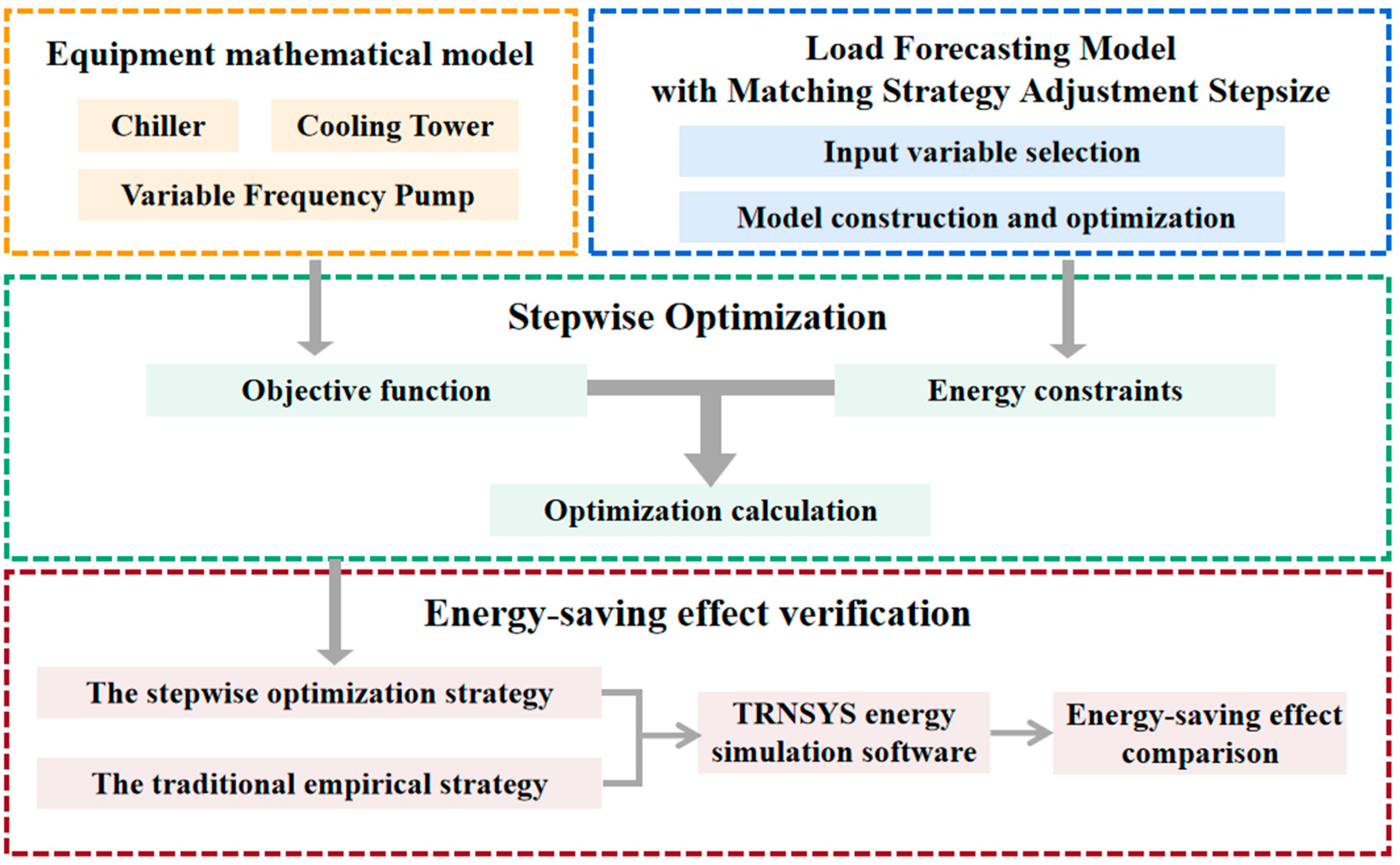
The technology roadmap of this study is shown in Figure 1. The rest of this paper is organized as follows: Section 2 describes the methodology, including the construction of mathematical models of the analyzed equipment, a load prediction model, and a stepwise optimization model. Then, a case analysis comparing the traditional empirical strategy and the stepwise optimization operation strategy is introduced in Section 3. Finally, this study’s conclusions are presented in Section 4.
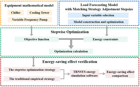
Figure 1.
Technical roadmap.
2. Materials and Methods
Before the optimization model could be developed, a mathematical model of the main equipment of the air-conditioning system and a load prediction model needed to be established to provide the objective function and constraints needed for optimization. This section introduces the method for the construction of a mathematical model of the central air-conditioning system’s equipment, and then constructs a load prediction model with matching strategy adjustment steps. Based on the equipment-oriented mathematical model and the load prediction model, a stepwise optimization model of the group control system of the chiller room is developed.
2.1. Data Preprocessing
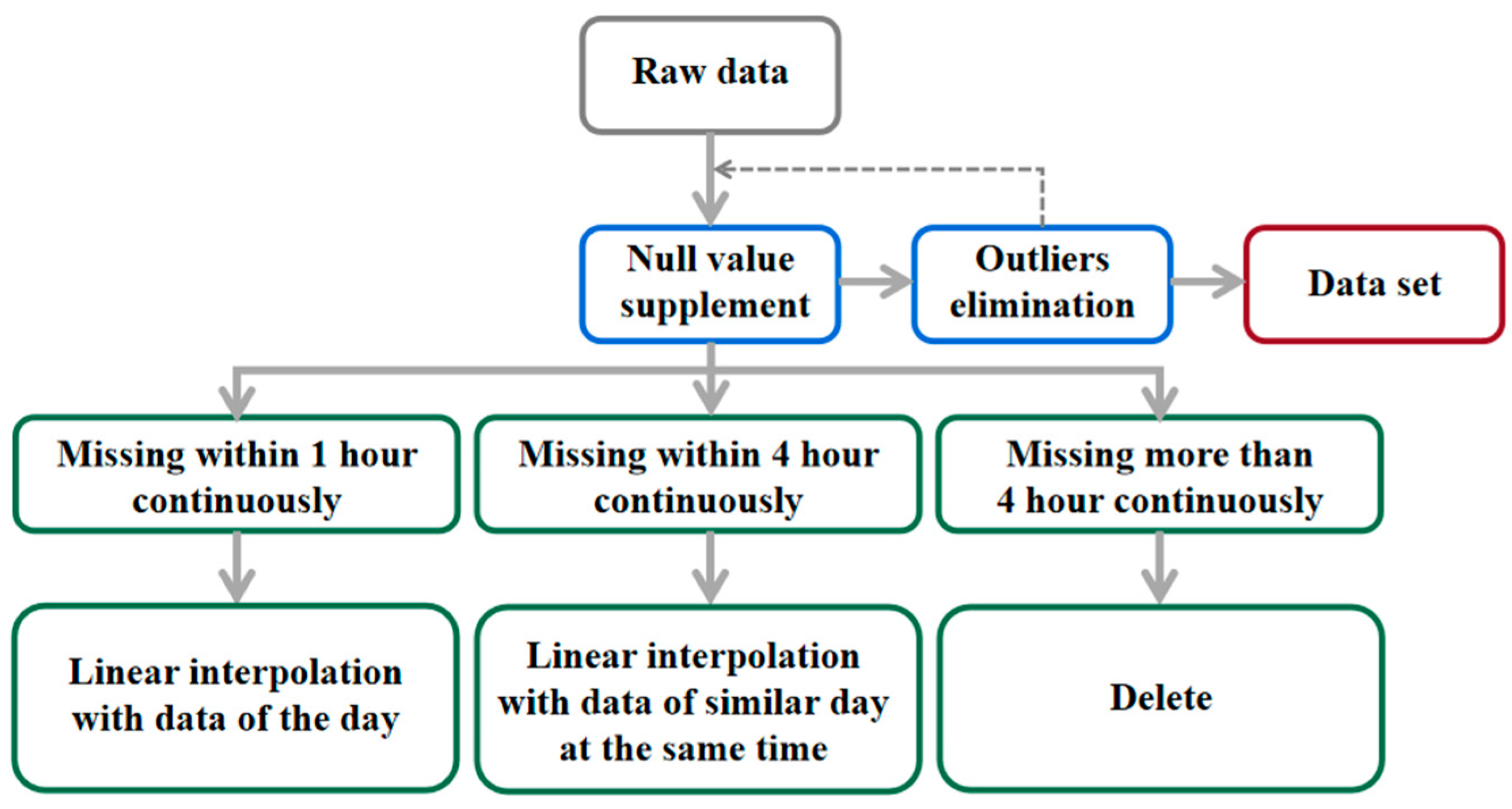
There are often missing data and outliers in the raw data obtained from indoor temperature-monitoring systems and building automation systems. Therefore, data preprocessing is required, which is shown in Figure 2.

Figure 2.
Data preprocessing flow chart.
The building cooling load data are calculated by the combination of three parameters: chilled water flow, chilled water supply temperature, and return temperature (see Equation (1)):
where C represents the specific heat capacity of water, M represents the flow rate of the heating circulation pump, Tg represents the temperature of supply water, and Th represents the temperature of return water.
In the formative process of a building’s cooling load, there is a time lag due to the thermal inertia of the building’s envelope and the complexity of the water system’s pipe network. In this paper, the time lag cross-correlation (TLCC) method is used to determine the delay time τ between supply and return water temperatures. TLCC method is performed by moving a time series vector in a stepwise manner and repeatedly calculating the correlation between two signals. If the peak value of correlation is at the center (offset = 0), this means that the two time series have the highest degree of correlation at this time. During data processing, the moving time step is 5 min.
As shown in Figure 3, the correlation of the chilled water return temperature is highest when the delay time τ is 20 min. Therefore, τ is taken to be 20 min. To a certain extent, these data can be regarded as the lag time of the water system’s circulation, which means that the temperature difference between the supply and return water after 20 min can be used for the load calculation at the current moment.
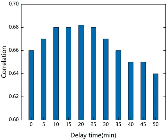
Figure 3.
TLCC calculation results.
2.2. Equipment Mathematical Model
This paper focuses on the energy-saving optimization of the equipment in the chiller room. The equipment involved in the machine room group control system includes the cooling tower, chiller, cooling water pump, and chilled water pump.
2.2.1. Chiller Mathematical Model
Many scholars have studied the energy efficiency of chillers and proposed a series of chiller energy efficiency models, including temperature-dependent models [26], simple linear regression models [27], variable quadratic regression models [28], multivariable multinomial regression models [28], DOE-2 models [29], and so on. Considering that chiller energy efficiency has a strong correlation with the actual chiller load Qe, chilled water supply temperature Tchws, and cooling water return temperature Tcwr, and that these influencing factors can be expressed by mathematical variables, the chiller power model concerning Tchws, Tcwr, and Qe is selected with reference to ASHRAE’s HVAC application manual (see Equation (2)).
In Equation (2), Pc is the electric power of the chiller, while c0, c1, c2, c3, c4, and c5 are the parameters to be identified in the model.
The least squares (LS) method, recursive least square (RLS) method, and forgetting factor least square (FFLS) method are used for parameter identification of the mathematical model of the chiller. Root-mean-square error (RMSE) was used to assess the model’s accuracy. The coefficient of determination (R2) was used to evaluate the fitting degree of the model to the sample data. The higher the R2, the better the fit of the model, and the stronger the model’s ability to interpret the dependent variable.
In Equations (3) and (4), fi represents the model’s output value, yi represents the actual value, m represents the number of samples, and represents the actual average value of samples.
2.2.2. Cooling Tower Mathematical Model
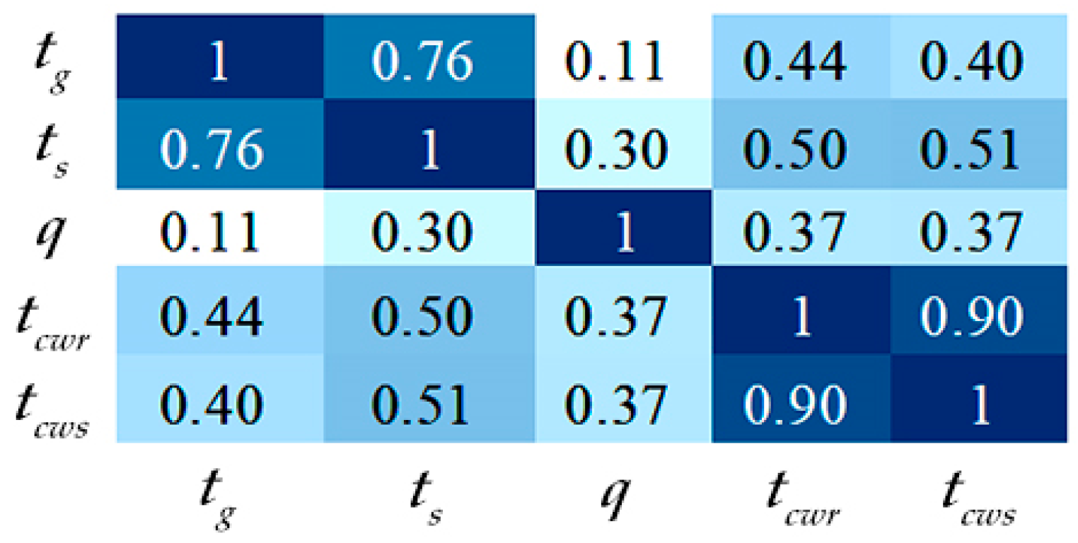
The energy transfer process of a cooling tower is very complex. Unlike water chillers and variable frequency pumps, there is no generally recognized and widely accepted numerical model of a cooling tower available in the industry. With reference to relevant research [30,31,32], this paper adopts the multiple linear regression model to numerically describe the cooling tower’s power. The cooling tower’s outlet water temperature is mainly related to the flow, the cooling water’s inlet temperature, and the fan’s operating frequency. In addition, this parameter may be related to meteorological factors. The Pearson correlation coefficient [33] method was used to conduct a correlation analysis on influencing factors of cooling water outlet temperature tcwr. The correlation analysis’s results obtained for the variables, including cooling tower’s inlet and outlet water temperature, the cooling water flow, and air wet and dry bulb temperature, are shown in Figure 4.

Figure 4.
Results of correlation analysis between influencing factors of cooling tower’s outlet water temperature.
The absolute values of the correlation coefficients were ranked. The correlations were ordered from highest to lowest: cooling tower inlet water temperature tcws, air wet bulb temperature ts, air dry bulb temperature tg, and cooling water flow rate q. Other factors with low correlation (absolute value below 0.3) were not included in the analysis. It should be noted that the correlation coefficient between dry and wet bulb air temperature is greater than 0.7, which indicates a strong correlation. Considering the higher correlation between the cooling tower discharge temperature and the air wet bulb temperature, and since ts is generally used to assess the capacity of the cooling tower, tg is not considered. The cooling tower energy consumption model was developed as shown in Equations (5) and (6). Equation (5) represents the relationship between the cooling tower outlet water temperature and fan’s operating frequency. Equation (6) describes the relationship between fans’ energy consumption and operating frequency.
In the equations above, P is the energy consumption of the fan, f is the cooling tower fan’s operating frequency, and f0 is 50 Hz. The least squares (LS) method, recursive least squares (RLS) method, and forgetting factor least squares (FFLS) method are used for parameter identification of the mathematical model in Equation (5). The other equation in the model only has three variables, whose determination is relatively simple, and the least squares method is used to identify these parameters.
2.2.3. Water Pump Mathematical Model
For the cooling water pump and chilled water pump models, this paper refers to the principle of variable frequency pump modules in TRNSYS energy consumption simulation software.
The model mainly explains three key points of variable frequency pumps: (1) the relationship between pump head and flow, that is, the pump’s operating conditions; (2) the relationship between pump efficiency and flow variation, that is, the pump’s efficiency curve; and (3) the pump’s power, that is, the pump’s energy consumption under different working conditions.
First, the sample curve is fitted with reference to the pump sample. Then, the change rule describing the pipe network’s impedance is analyzed through actual operation data. The air-conditioning unit and fresh air unit were activated in advance during normal working hours, and this did not affect the pipe network’s impedance. The activation and deactivation of fan coil units are set by users, which is the main reason for the change in pipe network impedance during working hours. Based on this, according to the pipe network impedance in different periods of working hours on weekdays, the operating state parameters of pumps can be solved. The calculation formula for pipe network’s impedance is shown in Equation (7). H refers to the pump’s head and q refers to the pump’s flow.
when the cooling water pump operates with variable frequency, the factor that may cause the impedance change in the whole pipe network is solely the frequency converter. The average impedance of the cooling water pipeline under the operating conditions of typical working days at different frequencies is determined. If the change rate of pipe network impedance is very small in the process of frequency reduction, an appropriate step size can be taken, and the impedance between the steps is averaged.
The commuting time of common public buildings is around 8:00–18:00, and the indoor air conditioner in the office area is kept on during daytime working hours. The fan coil is generally started around 8:00–9:00. From 17:00 to 18:00, the fan coil units are closed successively. During the commuting period, all the fan coil units essentially remain open. Considering the model’s universality in terms of actual projects, the impedance of the chilled water pipe is ascertained by determining the average fixed value at different sections of time.
In addition, since the impedance change of the pipe network caused by the opening and closing of the fan coil is far greater than that caused by the frequency converter, in the special time nodes of on and off duty, the influence of the pump’s operation frequency on pipe network impedance is not considered, and the average value of the time nodes in a typical week can be selected.
2.3. Load-Forecasting Model with Matching Strategy Optimization Step Size
The main function of load forecasting is to provide energy constraints for the optimization of group control strategies in chiller rooms. In this paper, the chiller’s cooling capacity is selected for use as the load data. The time lag of the water system was determined to be 20 min by the TLCC method. During the chiller’s start-up phase, the indoor temperature was in the process of dropping from a higher level to a comfortable range, which does not mean that the cooling capacity is sufficient to maintain a comfortable indoor temperature at that moment. The period between 7:30–9:00 in the chiller’s startup phase was not considered, while the indoor temperature between 9:00–18:00 was basically maintained at a comfortable range, and its cooling capacity can represent the cooling load. Therefore, the load-forecasting model only forecasts the load data of the building from 9:00 to 18:00 every day, and the forecasting step is 15 min. In addition, the load-forecasting model needs to provide the next load forecasting value every 15 min and optimize the operation parameters to meet this load value.
2.3.1. Input Variable Selection
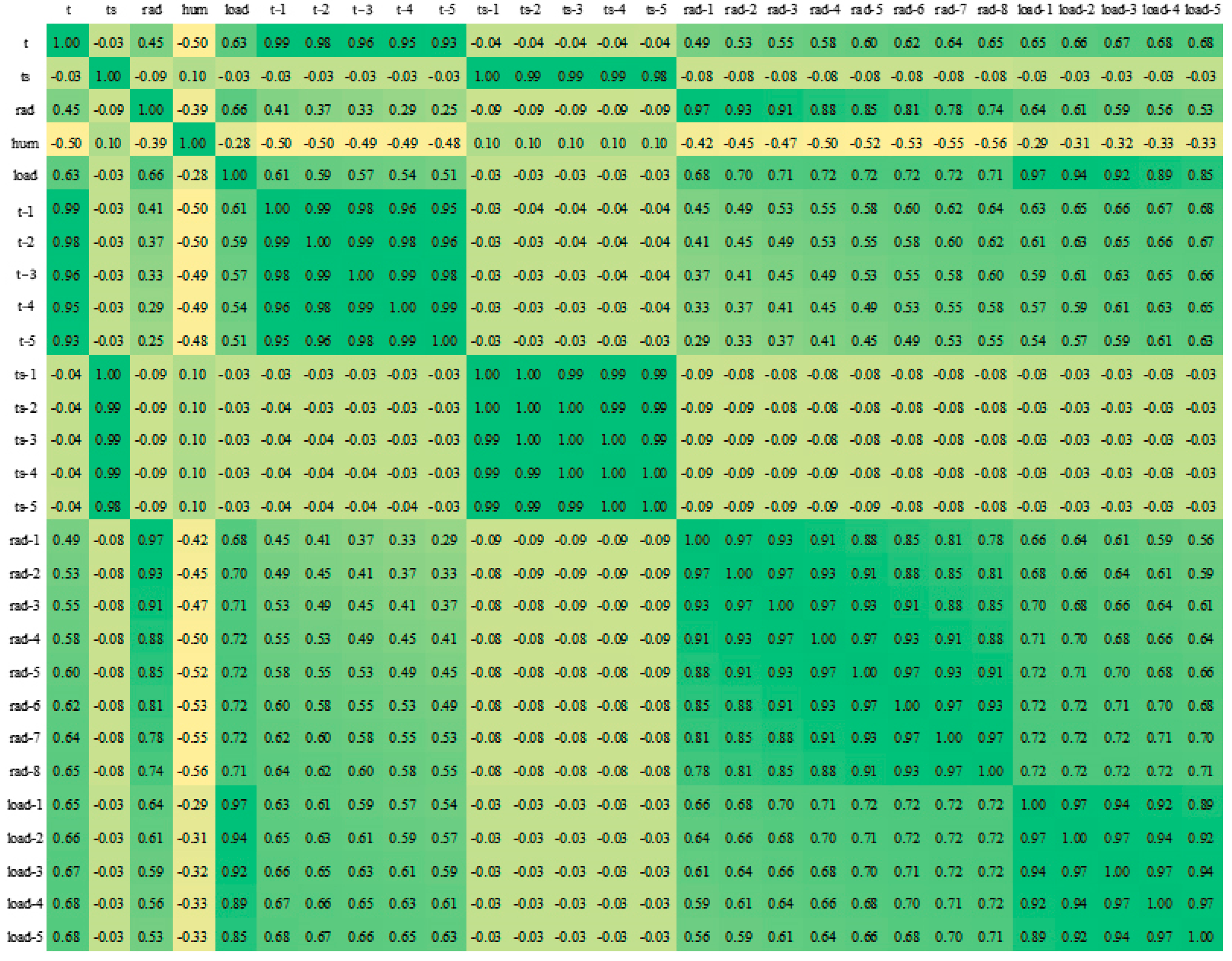
Firstly, the Pearson method is used to analyze the correlation between the influencing factors of the building’s cooling load. For climatological factors such as temperature, humidity, and solar amplitude intensity, the building’s cooling load is influenced by these outdoor weather data and their previous n time intervals (n is taken as 24 in this paper). To facilitate the presentation of each datatype, only the first five time intervals were developed into a thermodynamic diagram. The results are shown in Figure 5.
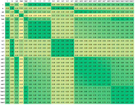
Figure 5.
Results of correlation analysis between influencing factors of building cooling load.
In Figure 5, t represents dry bulb temperature, ts represents wet bulb temperature, rad represents total radiation, hum represents relative air humidity, and load represents building’s cooling load, while t−1 denotes dry bulb temperature at the previous one-time interval, t−2 denotes dry bulb temperature at the previous two-time interval, and so on. 1 time interval corresponds to 15 min.
Sort the absolute values of load correlation. When the correlation coefficient is greater than 0.3, the correlation is considered strong. However, too many and too similar input variables will increase the number of redundant calculations carried out by the model and may lead to overfitting. Therefore, t, t−1, t−2, t−3, rad-5, rad-6, rad-7, load-1, load-2, and load-3 are included as input variables.
With regard to the internal disturbance caused by user behavior, the corresponding power branch is selected, and Pearson correlation analysis is conducted concerning the power branch and load of lighting and equipment. The average value of three branches with a strong correlation is selected to replace the rule governing personnel density change.
2.3.2. Model Construction and Optimization
The ensemble learning method was selected to build a load-forecasting model. There are many algorithms that use multiple learners to complete the learning task. In this paper, the Random Forest (RF) algorithm was selected.
To match the step size of the stepwise strategy optimization method, the data from 9:00–18:00 each day are selected, and the data with an interval of 15 min are extracted to form an overall dataset after preprocessing. Through the above analysis, the model’s input variables are outdoor dry bulb temperature of the previous 15, 30, and 45 min; total solar radiation of the previous 15, 30, and 45 min; the load of the previous 15, 30, and 45 min; and internal disturbance. The output variable is the current load.
This model is applied to predict the building’s load after 15 min in the actual prediction task. In fact, the input data will not change suddenly in a short time interval. Taking the outdoor temperature as an example, the average dry bulb temperature change within 15 min is 0.4, which can essentially be regarded as unchanged, and the same is true for other data. Therefore, in the actual task, the actual data at time t will be used as the input variable to predict the output at time t + 15 min. The ratio of the training set, test set, and validation set is 7:2:1. The test set is used to adjust parameters, and the verification set is used to evaluate the model performance. During initial training of the model, all hyper-parameters are selected as default values. After ensuring that the code can run normally, the GridSearchCV method is used to optimize the hyperparameter.
2.4. Stepwise Optimization
The equipment in the chiller room is divided into the chiller side and the cooling side according to their functions. The two sides of the system are optimized sequentially. The chilled side includes chiller and chilled water pump, while the parameters for optimal control are chilled water supply temperature and chilled water flow. The cooling side includes the cooling tower and cooling water pump, while the parameters for optimal control are the cooling water outlet temperature and the cooling water flow. This section will establish the stepwise optimization model with objective functions and constraints for both sides according to the equipment power model and the load prediction model established previously.
2.4.1. Chilled Side
The objective function on the chilled side is employed to keep the sum of the energy consumption of the chiller and chilled water pump to a minimum (see Equation (8)).
The subscript ch is the abbreviation of chiller, representing the parameters related to the chiller, and the subscript chp is the abbreviation for chilled water pump, representing the parameters related to it, which are used in the following text. In Equation (8), P represents the power, Pch refers to the chiller power, and Pchp refers to the chilled water pump power.
When optimizing constraints, both equipment performance constraints and energy constraints should be considered. The premise behind achieving the optimal control of an air-conditioning system is to ensure both the stable operation of the system and that the operating parameters of each piece of equipment change within a reasonable range. If the result calculated by the model exceeds the normal threshold, the optimization result is meaningless. Therefore, it is necessary to constrain the equipment’s operating parameters. According to the equipment performance and expert knowledge, the chilled water supply temperature was set at 5–11 °C. The range set for the chilled water return temperature was 6–15 °C. The operating frequency of the chilled water pump was limited to 30–50 Hz. The power limits of the chiller and chilled water pump were determined by referring to the historical operation data and equipment specifications of the whole cooling season.
The chilled water return temperature should be corrected after each optimization. Under similar operating conditions, the temperatures are extracted and sorted, and the maximum value is taken as the limit of chilled water return temperature at that moment. If the parameters’ combination at the optimization moment is within the allowable deviation from the parameters’ combination at a certain moment in time, the moments are considered to be similar.
The cooling capacity provided by the chiller room, which was calculated as shown in Equation (9), needs to be able to satisfy the terminal environmental load demand from the load-forecasting model, which is the fundamental condition for ensuring the comfort of the resulting environment.
In Equation (9), C represents water’s specific heat capacity, taken as 4.2 × 10³ J/(kg·°C); M represents the mass flow of chilled water; tchws represents the chilled water supply temperature; and tchwr represents the chilled water return temperature. In a previously built variable frequency pump model, the flow and pump frequencies could be calculated.
In conclusion, the constraint values of each parameter on the chilled side are shown in Table 1.

Table 1.
Range of constraint variables on the chilled side.
2.4.2. Cooling Side
The objective function of the cooling side is employed to minimize the sum of energy consumption of the cooling tower, chiller, and cooling water pump.
The subscript ct is the abbreviation for the cooling tower, representing the parameters related to the cooling tower, and the subscript cp is the abbreviation for the cooling water pump, representing the parameters related to the cooling water pump, which are explained as follows: P represents power, Pch refers to the chiller’s power, and Pcp refers to the cooling water pump’s power.
The analysis of constraints on the cooling side is basically the same as that applied to the chilled side. The constraint values of the parameters on the cooling side are shown in Table 2.
Table 2.
Range of constraint variables on the cooling side.
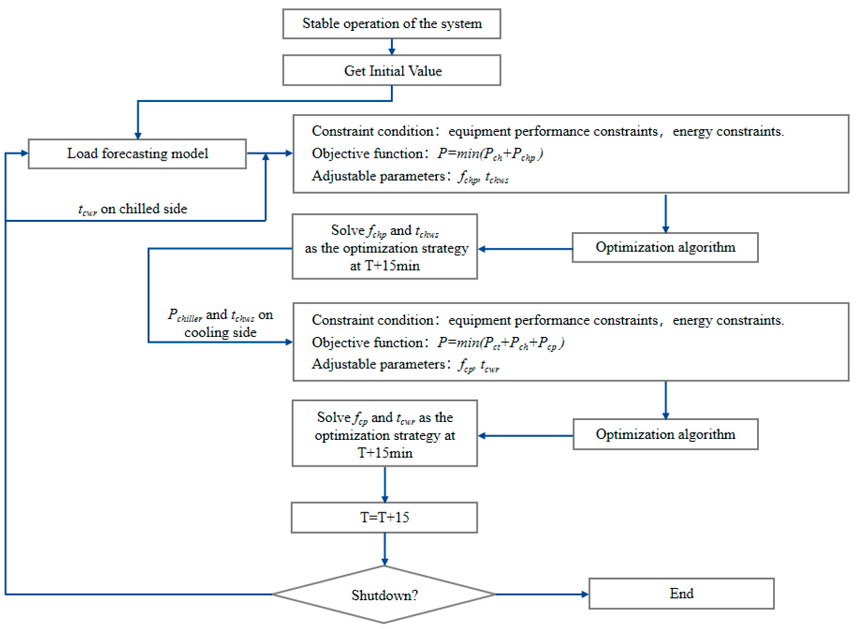
2.4.3. Stepwise Optimization Implementation
The calculation process of the stepwise optimization model is shown in Figure 6. When the system starts to work stably (9:00–18:00), the operation strategy of T + 15 min is optimized at moment T.
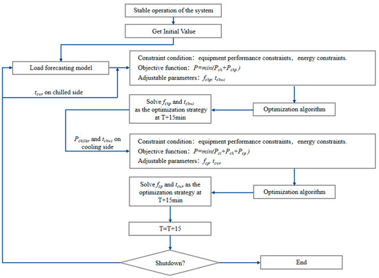
Figure 6.
Calculation process of the stepwise optimization model.
First, the chilled side is optimized. The initial values of the main parameter are fetched at moment T. The initial meteorological data are used as input values for the building load prediction model to obtain load data for the next moment. Based on the objective function and constraints, the chilled side strategy at the next moment is obtained through optimization.
Next, the initial chiller power, initial wet bulb temperature, chilled water supply temperature, and load prediction data are read and passed to the cooling side. The initial chiller power and predicted load values provide energy constraints for cooling side’s optimization. The initial wet bulb temperature data constitute an important input variable for the power calculation of the cooling tower. After the input conditions are defined, the cooling side parameters are optimized to obtain the cooling side optimization strategy for the next moment. Thus, one round of overall optimization will have been completed.
Continue with the next round of optimization, where the initial values are updated moment by moment with the results of the latest load prediction and the changes in meteorological data and chiller power.
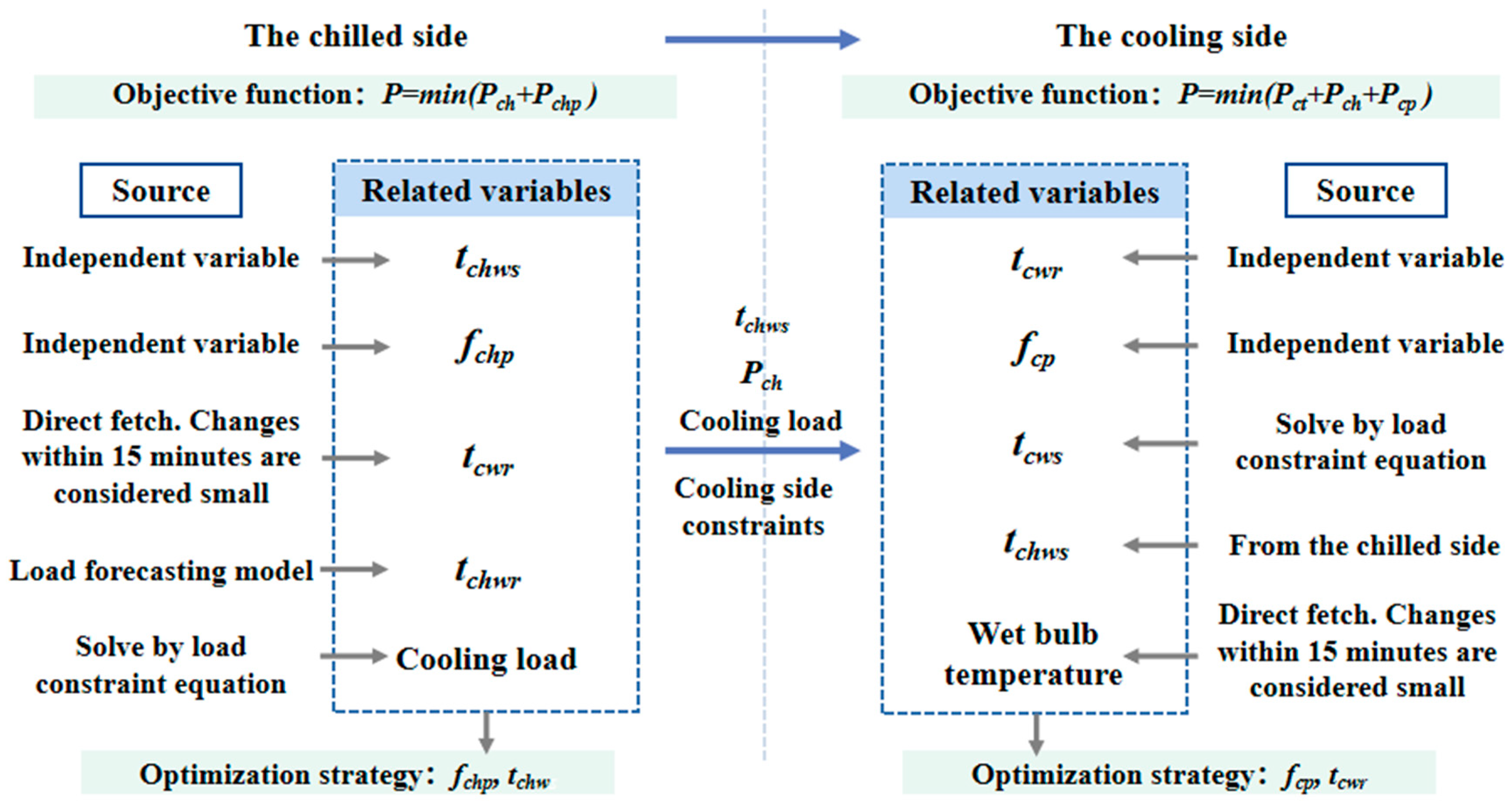
The variable selection issue involved in the optimization process on both sides is shown in Figure 7. After several attempts, the optimization results obtained when moving from the chilled side to the cooling side are basically the same as those from the cooling side to the chilled side. Therefore, the two processes are not introduced individually. The case studies in the later sections all use the optimization process from the chilled side to the cooled side.
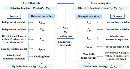
Figure 7.
Variable value method.
3. Case Analysis
The TRNSYS energy simulation software is used to construct a model of the central air-conditioning system of the analyzed building. The traditional empirical strategy and the stepwise optimized operation strategy are compared in the same experimental environment.
3.1. Simulation Set-Up
An office building in Beijing, China, was taken as an example, with a building area of 95,000 m2 and a height of 68.50 m, including 17 floors above ground and 2 floors underground. The working hours of the office area in the building are from 8:00 to 18:00. The designed cooling load of the air-conditioning system is 9142 kW. There are four centrifugal chillers with a cooling capacity of 2286 kW per unit. The chilled water system is a variable flow secondary pump system with four primary chilled water pumps with a rated power of 75 kW. Three chilled water secondary pumps have 75 kW of motor power, 32 m of head, and a 55 m3 flow rate. Four cooling water pumps have 75 kW of motor power, 34 m of head, and a 470 m3 flow rate. The chilled water secondary pump and cooling water pump have variable frequency control. Four cooling towers are installed on the top of the north building with a rated current of 8 A and a water flow rate of 200 m3/h. The data set for this study contains operational data concerning this building for the entire duration of the 2021 cooling season, which spanned from 21 June to 28 September. Based on the data set, parameter identification or pipe network impedance calculation was carried out to obtain the mathematical models of the chiller, cooling tower, and variable frequency water pump mentioned above.
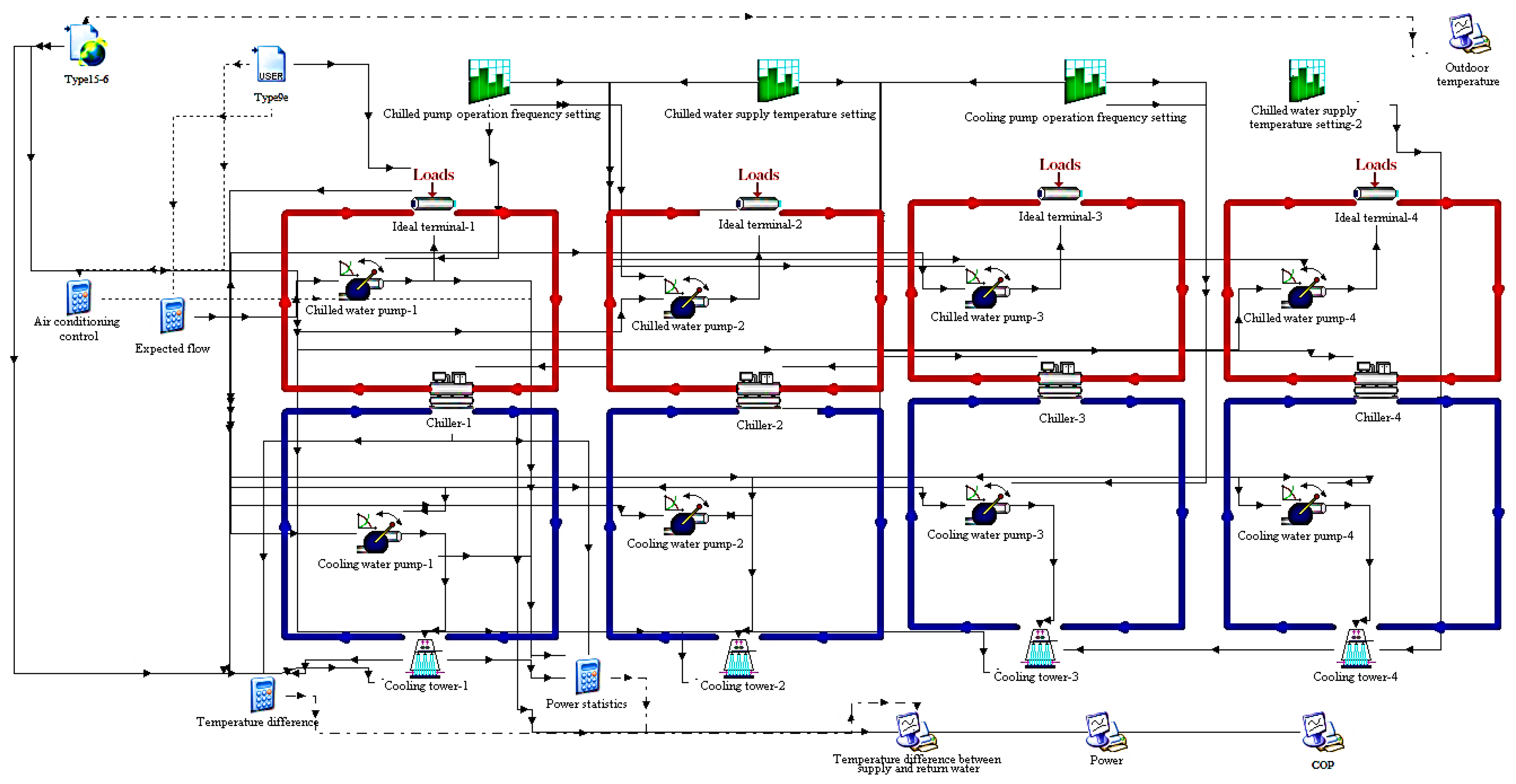
The cold season equipment system model was developed in Simulation Studio with reference to the plane figure and system diagram of the machine room of the central air-conditioning system in the building. The main types of energy-consuming equipment are the chillers, cooling water pumps, chilled water pumps, and cooling towers. In the TRNSYS energy consumption model, the ideal resistance-free end was generally adopted, and the concept of the primary pump overcoming the resistance of the machine room and the secondary pump overcoming the resistance of the pipe network outside the machine room is not considered. In addition, the flow-matching problem of the primary and secondary pumps is complex, so no primary pump was rendered in the simulation process, and the flow data can be directly used by the secondary pump flow. The step size of the simulation was set to 15 min. The simulation model is shown in Figure 8.
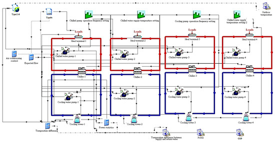
Figure 8.
TRNSYS energy consumption simulation model.
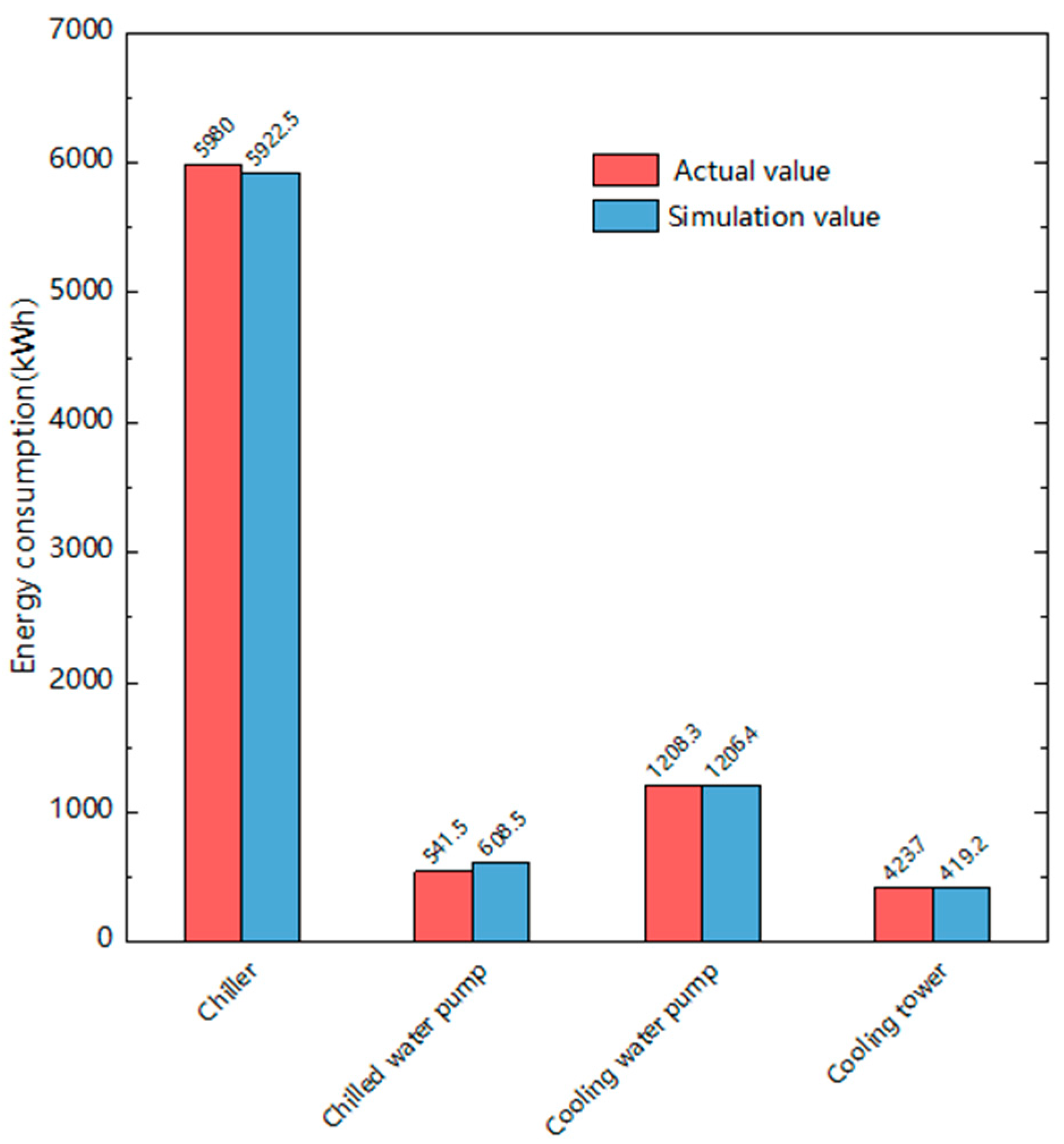
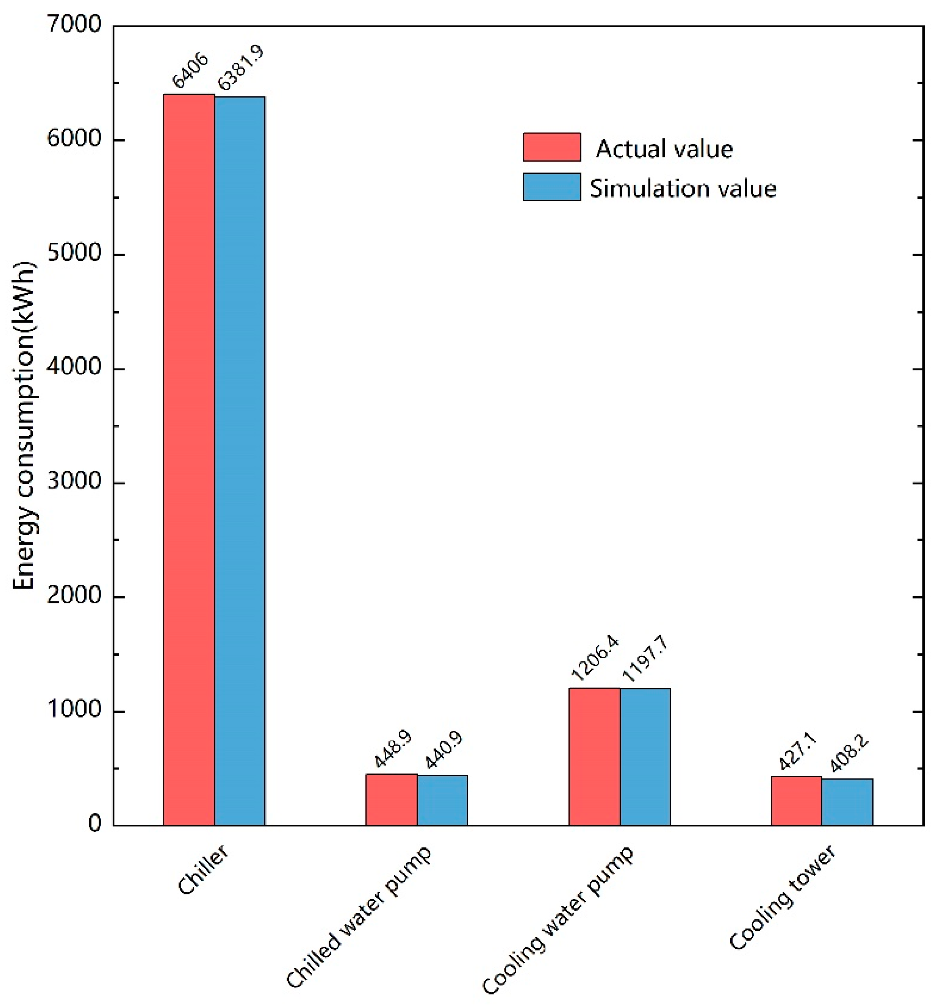
After the model was built, the simulation model was set according to the nameplate parameters of actual engineering equipment to assure that the model could realistically reflect the operation of the buildings to a certain extent. The operation data from two randomly selected days, 3 August and 5 August, were used as examples to verify the operating power of the chiller, chilled water pump, cooling water pump, and cooling tower. The calculation results are shown in Figure 9 and Figure 10. The relative errors of the calculated results for the two days are 0.96% and 0.37%, respectively. The relative errors are 12.4% and 1.7% for the chilled water pump power, 0.15% and 0.7% for the cooling water pump, and 1.1% and 4.4% for the cooling tower, respectively. From an engineering perspective, relative errors below 15% are acceptable, so the simulation model can be used to simulate system operations.

Figure 9.
Model validation results on 3 August.

Figure 10.
Model validation results on 5 August.
3.2. Comparison of Optimization Strategies
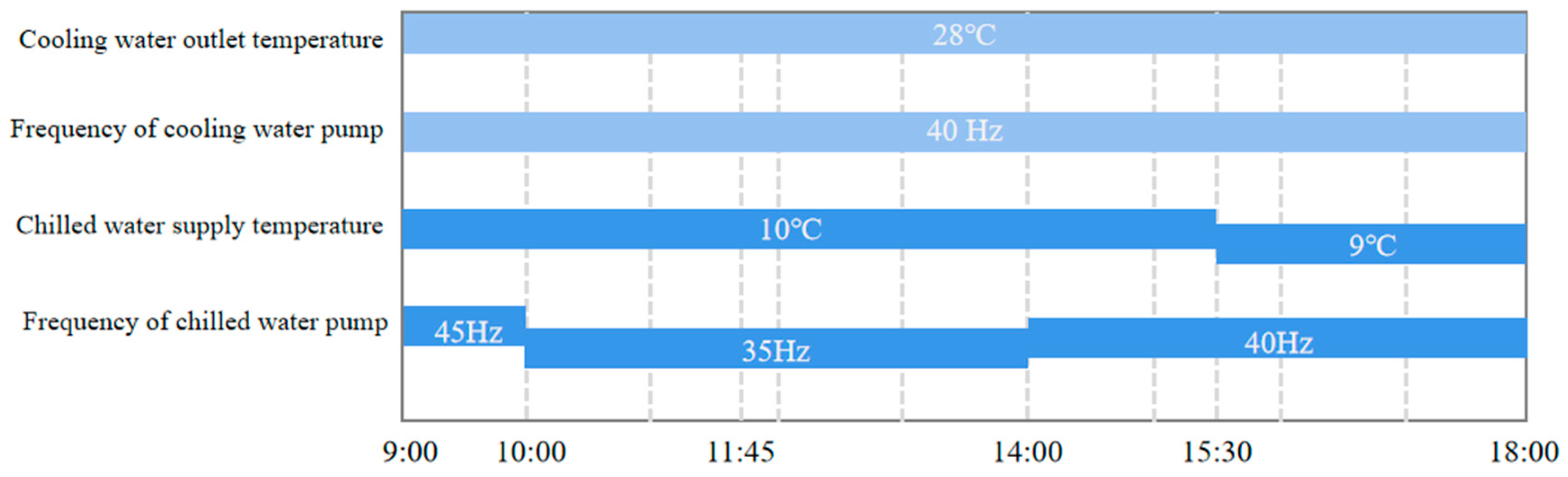
Without considering special weather, one day was selected for analysis on a weekday when two chillers were running throughout the day and on a weekday when one to two chillers were switching operation throughout the day. The weekdays of 16 July and 9 August were randomly selected. On 16 July, two chillers were in operation until 11:45; after this point, only one chiller was in operation. On 9 August, two chillers ran throughout the day.
As shown in Figure 11, the studied building’s cooling side operation strategy was not adjusted throughout the day on 16 July. The outlet temperature of the cooling water was 28 °C and the cooling water pump’s operating frequency was 40 Hz. Before 10:00, the cooling capacity was too great, so the chilled water pump operating frequency was reduced from 45 Hz to 35 Hz. At 11:45, the cooling capacity was still too great, so one chiller was shut down. After 15:00, it was found that the cooling capacity was insufficient, so the chilled water pump’s operating frequency was increased to 40 Hz, and the water supply temperature was reduced to 9 °C.
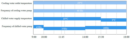
Figure 11.
Traditional empirical operation strategy on 16 July.
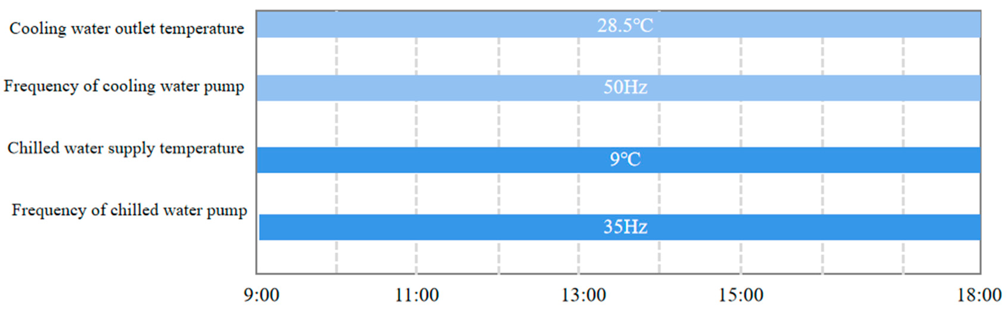
As shown in Figure 12, on 9 August, the operation strategy of the studied building was adjusted. This building’s operation strategy for the day is consistent with that of most public buildings. The staff sets the strategy of the next day based on weather prediction data and personal experience. It can be seen that if the room temperature does not deviate excessively, the strategy is not adjusted throughout the day.
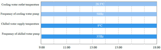
Figure 12.
Traditional empirical operation strategy on 9 August.
The actual operating conditions of the building on 16 July and 9 August were input into the stepwise optimization model. The results of the two days’ strategy optimization are shown in Table 3 and Table 4, respectively. Due to the large number of data, the time interval of the data displayed after 11:00 in Table 3 and Table 4 is 1 h.
Table 3.
Comparison of two strategies on 16 July.
Table 4.
Comparison of two strategies on 9 August.
A comparison of the two strategies reveals the following:
- (1)
- The traditional empirical strategy is as follows: if the rooms are not too cold or too hot, the equipment’s operation parameters are not adjusted throughout the day. It can be seen that there is a delay in the adjustment behavior of managers. The adjustment concerning the alteration of the cooling capacity on the chilled side was employed after problems occurred in the terminal room. This adjustment was executed blindly, and the strength of the adjustment was based on experience without scientific guidance. So, the adjustment was attempted several times during the day. This will negatively affect the terminal environment comfort, the energy-efficient operation of HVAC systems, and even the working capacity of the property’s HVAC team. Secondly, the adjustment process entails the disconnection of the equipment. Heat dissipation on the cooling side does not match the building’s load and the cooling machine’s heat dissipation, which readily leads to energy waste and the depreciation of equipment’s operational life.
- (2)
- The stepwise optimization strategy realizes the goal of the dynamic adjustment of the system with the real-time load as the target. To offset the additional load generated by activating the fresh air unit after 10:00, a strategy to lower the chilled water supply temperature setting was adopted. After restoring stability, the water supply temperature and the flow rate increased. In this process, the optimal solution is always tracked for different working conditions. The cooling load is the dominant factor affecting strategy formulation. However, some highly relevant factors such as the wet bulb temperature of the cooling tower cannot be ignored. These factors occupy a certain weight in the stepwise optimization model and have not been taken into account by empirical strategies.
- (3)
- The empirical strategy on the chilled side favors a small flow rate with a large temperature difference. According to the calculation results, the variation in the energy consumption of the chiller caused by the chilled water supply temperature is much larger than that of the chilled pump caused by changing the chilled water flow. In this case, reducing the chilled water supply temperature in exchange for a large temperature difference is not an energy-saving strategy. Secondly, for large office buildings, the complex pipe network is prone to inferior loops. The use of a small flow supply will increase the temperature difference in different areas of the building.
3.3. Comparison of Energy-Saving Effects
The two operation strategies in the previous section were input into the TRNSYS model for comparison via simulation.
- (1)
- Energy consumption comparison on 16 July.
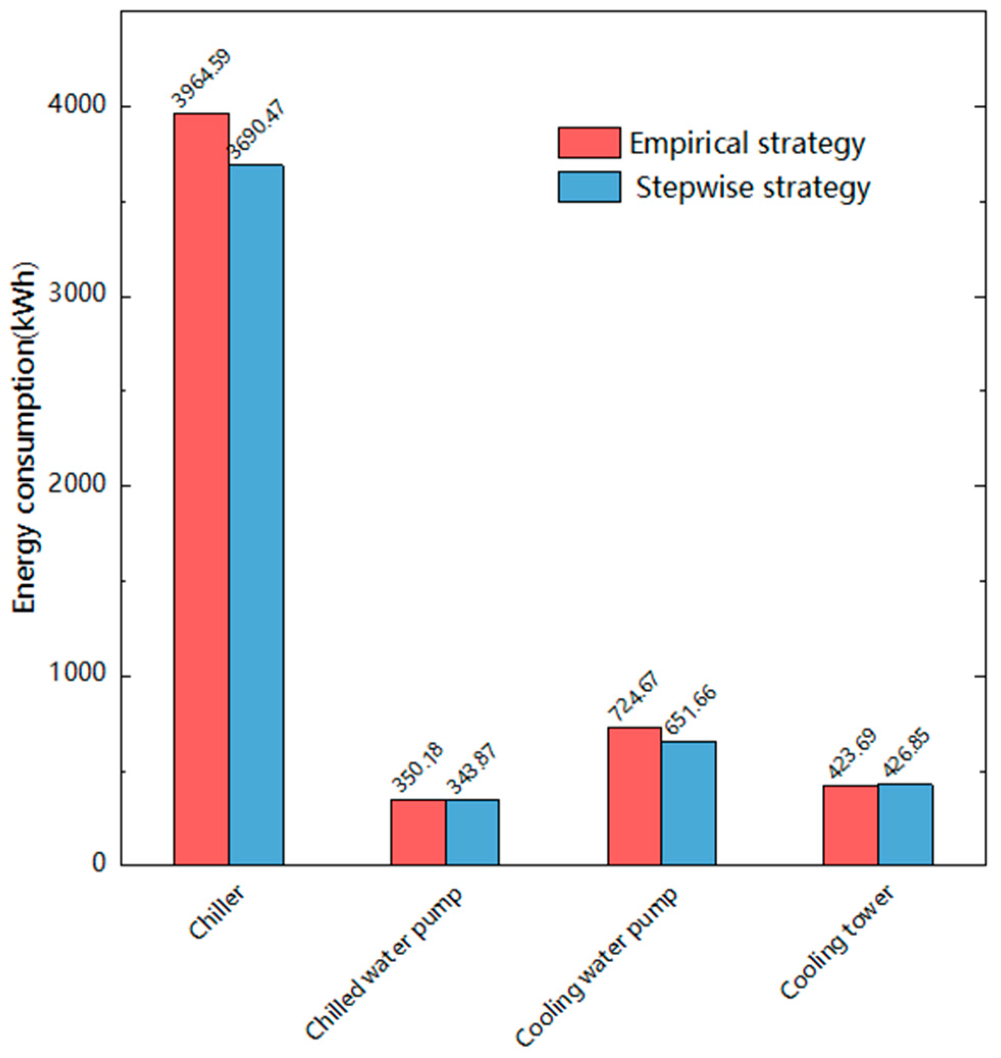
It can be seen from Figure 13 that the total energy consumption of the chiller throughout the day is much higher than that of the other three pieces of equipment; this value is followed by those of the cooling water pump, cooling tower, and chilled water pump (only the secondary frequency conversion pump). Among them, the chiller has the most obvious energy-saving effect. The energy consumption of the chilled water pump and the cooling tower is basically consistent under the two operation strategies. According to Table 5, the energy-saving rates of the chiller and cooling water pumps are 6.91% and 10.07%, respectively, and the total energy-saving rate is 6.41%. With the empirical strategy applied on July 16, the cooling capacity is greater than the actual load demand for part of the time, resulting in energy waste. There are also periods when the cooling capacity is less than the actual building load, during which the terminal environmental comfort is reduced, and the energy efficiency level of the equipment is low. Such a “positive and negative offset” led to a low energy efficiency level of the HVAC systems on that day.
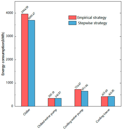
Figure 13.
Comparison of equipment energy consumption between the two strategies on 16 July.
Table 5.
Equipment energy consumption and saving rates obtained via the two strategies on 16 July.
Since both the chiller side and the cooling side contain chillers, there is a significant energy-saving effect on both sides. As shown in Table 6, the energy-saving rate is 6.50% for the chilling side and 6.73% for the cooling side. The energy-saving rates on both sides are practically the same.
Table 6.
Two sides’ energy consumption and saving rates via the two strategies on 16 July.
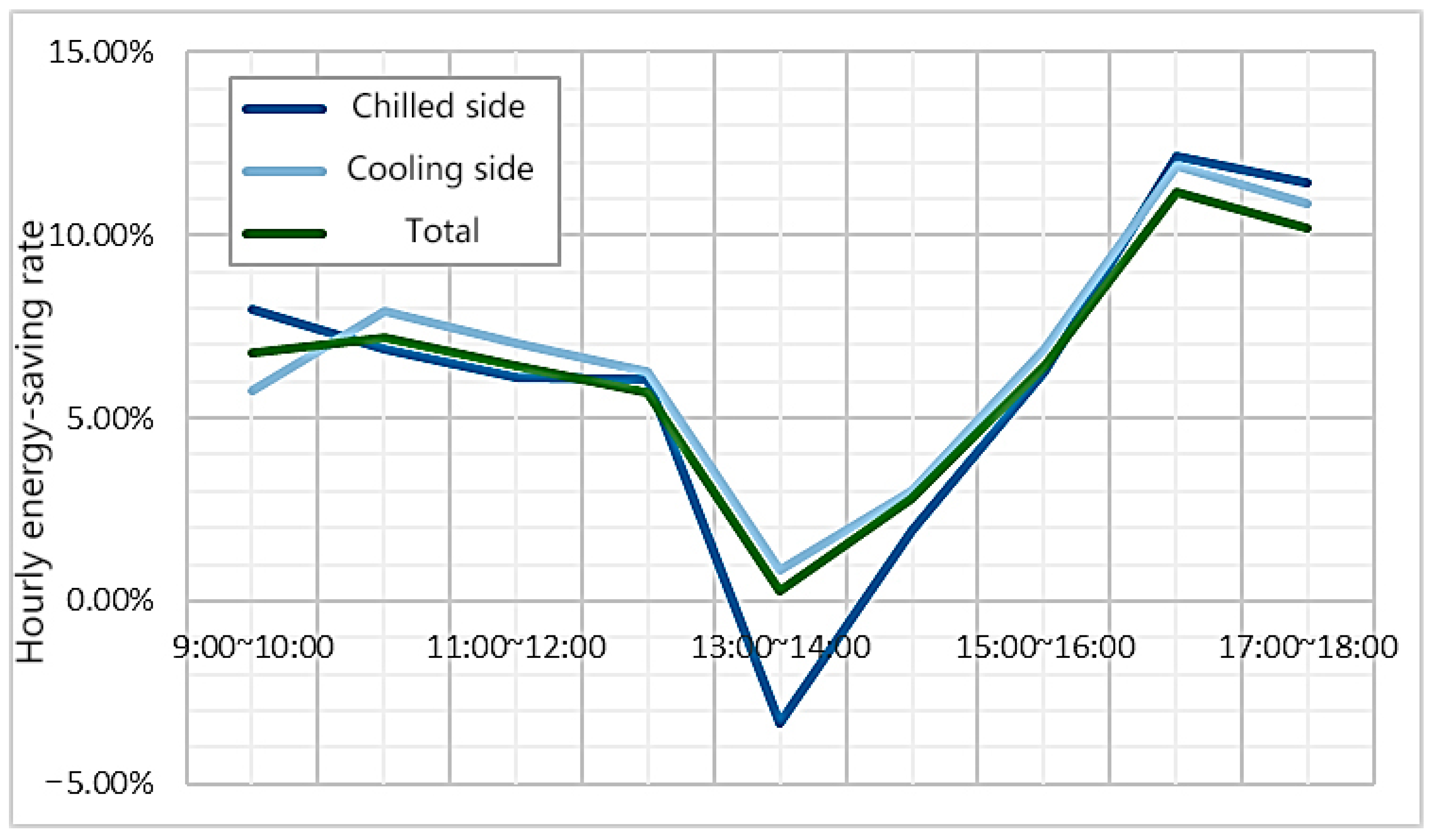
As seen in Figure 14, the main energy-saving periods during the system operation are concentrated between 9:00–12:30 and 15:00–18:00, and the energy-saving rate is greater than 5%. The highest energy-saving rate is from 16:00 to 18:00, and it was greater than 10%. To follow the load change in order to perform dynamic adjustment, the stepwise optimization strategy dictated setting the chilled water pump frequency 5 Hz higher than the empirical strategy during 13:00–14:00, which resulted in a negative energy-saving rate in the local period.
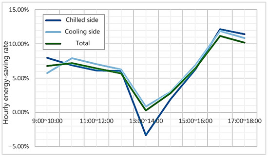
Figure 14.
Hourly energy-saving rate of chilled side and cooling side on 16 July.
- (2)
- Energy consumption comparison on 9 August
It can be seen from Figure 15 that the total energy consumption of the chiller throughout the day is much higher than that of the other three pieces of equipment, and this value is followed by the cooling water pump. The energy-saving effect of the chiller and cooling water pump is obvious. In combination with Table 7, the energy-saving rates of the chillers and cooling water pumps are all over 15%, the energy-saving rates of cooling towers are 5.62%, and the energy consumption of the chilled water pumps increases by about 15%.
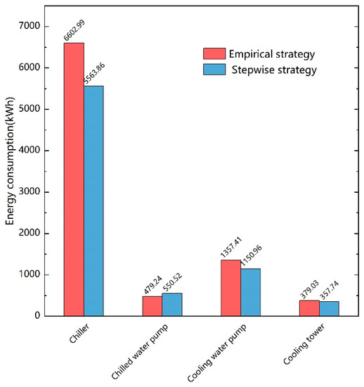
Figure 15.
Comparison of equipment energy consumption between the two strategies on 9 August.
Table 7.
Equipment energy consumption and saving rates obtained with the two strategies on 9 August.
The increased energy consumption of the chilled water pumps is inevitable. Empirical strategies employ the approach of providing chilled water at a 35 Hz frequency and 8 °C throughout the day, which obviously fails to grasp the main contradiction of the problem. The main share of energy consumption must be considered to achieve a greater energy-saving effect. However, the chillers and pumps with a large proportion of energy consumption offer the greatest energy-saving effect in the stepwise optimization strategy. Even if the energy-saving potential of the chilled water pump is lost, the whole-day energy consumption reduces by 13.56%.
As shown in Table 8, the energy-saving rates on the chilled side and the cooling side are 13.67% and 15.19%, respectively. Clearly, the cooling side has a high energy-saving potential, which is consistent with the conclusions of the previous analysis. On the analyzed day, the cooling water outlet temperature on the cooling side is set to low, while the cooling water pump runs at the rated frequency. Essentially, the maximum heat dissipation does not match the required heat dissipation, resulting in energy waste.
Table 8.
Two sides’ energy consumption and saving rates through the two strategies on 9 August.
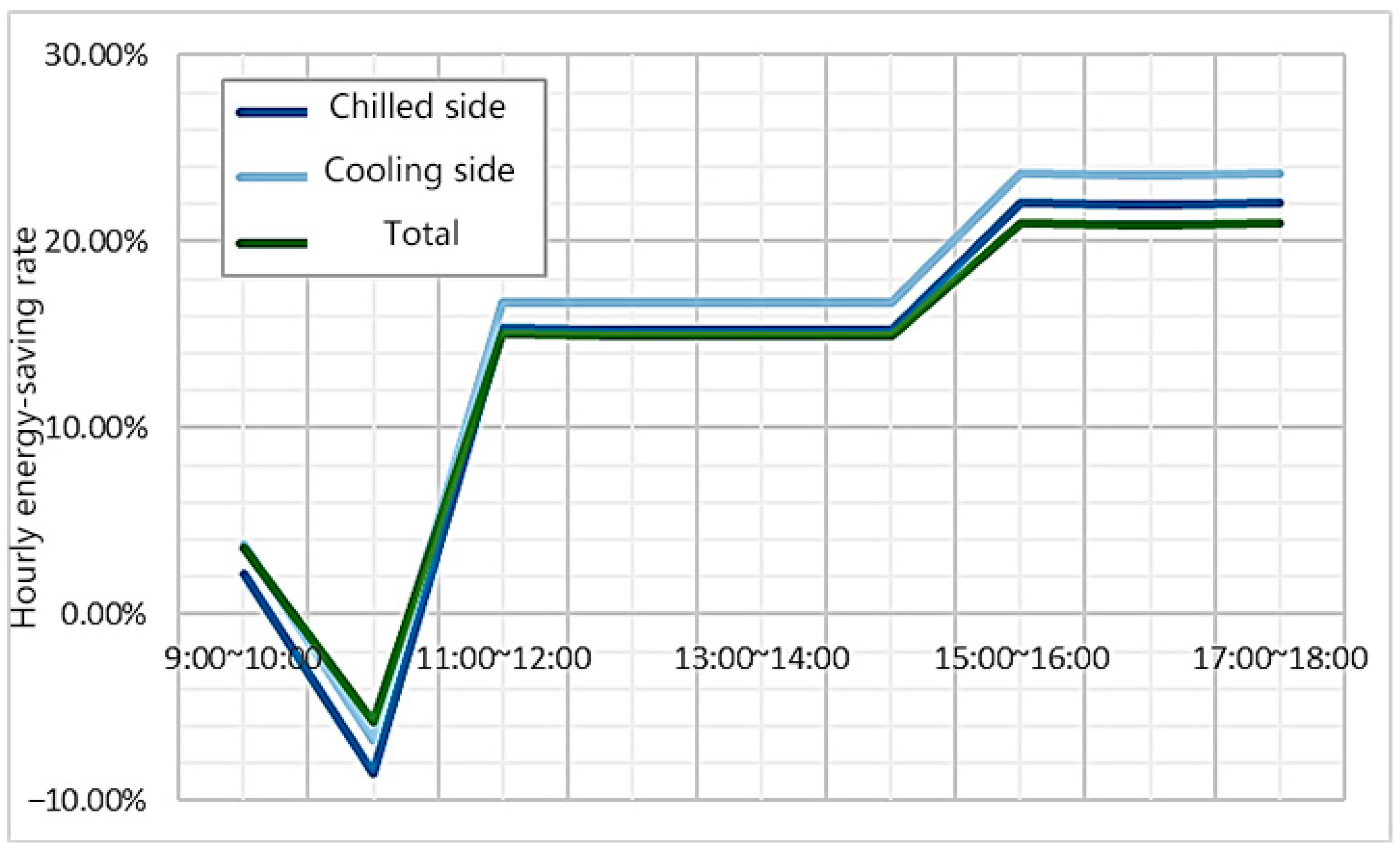
The hourly energy-saving rates are shown in Figure 16. The energy-saving rate per hour after 11:30 is above 15%, which is the main energy-saving operation time throughout the day. The building load is high from 10:00 to 11:00. In the process of the dynamic adjustment of the optimization strategy, the outlet temperature of the cooler is reduced to ensure the cooling supply, which results in high total energy consumption and a negative energy-saving rate.

Figure 16.
Hourly energy-saving rate of chilled side and cooling side on 9 August.
In conclusion, after adopting the stepwise optimization strategy, the energy-saving rates of the central air-conditioning system, refrigeration side, and cooling side are 6.41%, 6.50%, and 6.73%, respectively, throughout the work period on 16 July, and are 13.56%, 13.67%, and 15.19%, respectively, throughout the work period on 9 August. Thus, the energy efficiency of the stepwise optimization strategy has been verified.
4. Conclusions
There are many studies on the optimization of HVAC system operation strategies in the field of energy efficiency in public buildings. However, the fact that few of these studies have achieved effective and consistent performance in practical engineering applications is a problem. The effective implementation of optimization research in practical engineering is a problem commonly faced by researchers in this field. In this study, an innovative stepwise optimization method for central air-conditioning systems is proposed based on a summary of previous research results, with the objective of providing a new way of thinking regarding the optimization of operation policy. The main research processes and findings of this paper are summarized as follows:
- (1)
- The stepwise optimization method divides the central air-conditioning system into the chilled side and the cooling side, which reduces the number of devices in each optimization process. The optimal points of the two sides are obtained by stepwise sequential optimization calculations. Finally, the optimization results on both sides are integrated into the global optimization results.
- (2)
- A stepwise optimization model with reasonable objective functions, precise constraints, and a complete optimization process was developed. Equipment mathematical power models were selected to provide mathematical support for objective functions, and a short-term load prediction model with a matching strategy optimization step size was established to obtain the energy constraints.
- (3)
- Compared to the traditional empirical strategy, the stepwise optimization strategy realizes the goal of the dynamic adjustment of the system with the real-time load as the target, which allows operators to avoid the delay and error problems posed by manual adjustment.
- (4)
- Based on the TRNSYS platform, the stepwise optimization strategy and traditional empirical strategy are simulated, and their energy-saving effects are compared. In both cases of the two studied workdays, the energy-saving rates were 6.41% and 13.56%, respectively, which verifies the energy-saving capacity of the stepwise optimization strategy.
This paper presents work carried out on the optimization of the group control system of chiller rooms in public buildings. This optimization method results in the acquirement of the approximate optimal operating point of the system. It can be noted that the research findings of strategy optimization are often difficult to implement in practical buildings, which may be due to the low accuracy of the models used and the lack of complete and precise constraints. After all, the actual working conditions are very complex. The implementation of strategies in the actual projects still requires further exploration according to the real operational characteristics of the building under consideration.
Author Contributions
Conceptualization, X.W. and H.M.; methodology, X.W. and W.Y.; software, K.L.; validation, X.W. and W.Y.; formal analysis, X.W.; investigation, X.W.; data curation, K.L.; writing—original draft preparation, X.W.; writing—review and editing, W.Y. and X.Z. All authors have read and agreed to the published version of the manuscript.
Funding
This research was funded by the Opening Funds of State Key Laboratory of Building Safety and Built Environment & National Engineering Research Center of Building Technology, BSBE2022-01, and the Basic Research Program Projects in Qinghai Province, China in 2023, 2023-ZJ-738.
Data Availability Statement
Data are available upon request.
Conflicts of Interest
The authors declare no conflict of interest.
References
- Fan, C.; Xiao, F.; Zhao, Y. A short-term building cooling load prediction method using deep learning algorithms. Appl. Energy 2017, 195, 222–233. [Google Scholar] [CrossRef]
- Hong, T.; Yang, L.; Hill, D.; Feng, W. Data and analytics to inform energy retrofit of high performance buildings. Appl. Energy 2014, 126, 90–106. [Google Scholar] [CrossRef]
- Lee, J.U. IEA, World Energy Outlook 2020; Korea Electric Power Corporation: Naju-si, Republic of Korea, 2021. [Google Scholar]
- Jradi, M.; Veje, C.; JøRgensen, B.N. Deep energy renovation of the Mærsk office building in Denmark using a holistic design approach. Energy Build. 2017, 151, 306–319. [Google Scholar] [CrossRef]
- Noh, K.Y.; Min, B.C.; Song, S.J.; Yang, J.S.; Choi, G.M.; Kim, D.J. Compressor efficiency with cylinder slenderness ratio of rotary compressor at various compression ratios. Int. J. Refrig. 2016, 70, 42–56. [Google Scholar] [CrossRef]
- Li, H.; Wang, S. Coordinated optimal design of zero/low energy buildings and their energy systems based on multi-stage design optimization. Energy 2019, 189, 116202. [Google Scholar] [CrossRef]
- Sophie, N.; Mark, G.; Tom, L. A review of occupant-centric building control strategies to reduce building energy use. Renew. Sustain. Energy Rev. 2018, 96, 1–10. [Google Scholar]
- Marik, K. Advanced HVAC Control: Theory vs. Reality. IFAC Proc. Vol. 2011, 44, 3108–3113. [Google Scholar] [CrossRef]
- Harputlugil, T.; Wilde, P.D. The interaction between humans and buildings for energy efficiency: A critical review. Energy Res. Soc. Sci. 2020, 71, 101828. [Google Scholar] [CrossRef]
- Du, Y.; Zandi, H.; Kotevska, O.; Kurte, K.; Munk, J.; Amasyali, K.; Mckee, E.; Li, F. Intelligent multi-zone residential HVAC control strategy based on deep reinforcement learning. Appl. Energy 2021, 281, 116117. [Google Scholar] [CrossRef]
- Feng, W.; Wei, Z.; Sun, G.; Zhou, Y.; Zang, H.; Chen, S. A conditional value-at-risk-based dispatch approach for the energy management of smart buildings with HVAC systems. Electr. Power Syst. Res. 2020, 188, 106535. [Google Scholar] [CrossRef]
- Lu, L.; Cai, W.; Soh, Y.C.; Xie, L.; Li, S. HVAC system optimization-condenser water loop. Energy Convers. Manag. 2004, 45, 613–630. [Google Scholar] [CrossRef]
- Zhao, T.; Zhang, J.; Ma, L. On-line optimization control method based on extreme value analysis for parallel variable-frequency hydraulic pumps in central air-conditioning systems. Build. Environ. 2012, 47, 330–338. [Google Scholar]
- Ma, K.; Liu, M.; Zhang, J. Online optimization method of cooling water system based on the heat transfer model for cooling tower. Energy 2021, 231, 120896. [Google Scholar] [CrossRef]
- Chen, C.L.; Chang, Y.C.; Chan, T.S. Applying smart models for energy saving in optimal chiller loading. Energy Build. 2014, 68 (Pt. A), 364–371. [Google Scholar] [CrossRef]
- Wijaya, T.K.; Alhamid, M.I.; Saito, K.; Nasruddin, N. Dynamic optimization of chilled water pump operation to reduce HVAC energy consumption. Therm. Sci. Eng. Prog. 2022, 36, 101512. [Google Scholar] [CrossRef]
- Ma, Z.; Wang, S. Energy efficient control of variable speed pumps in complex building central air-conditioning systems. Energy Build. 2009, 41, 197–205. [Google Scholar] [CrossRef]
- Gao, D.C.; Wang, S.; Sun, Y. A fault-tolerant and energy efficient control strategy for primary–secondary chilled water systems in buildings. Energy Build. 2011, 43, 3646–3656. [Google Scholar] [CrossRef]
- Xiong, W.; Wang, J. Minimizing Power Consumption of an Experimental HVAC System Based on Parallel Grid Searching. Energies 2020, 13, 2083. [Google Scholar] [CrossRef]
- Vakiloroaya, V.; Samali, B.; Madadnia, J.; Ha, Q.P. Component-wise optimization for a commercial central cooling plant. In IECON 2011-37th Annual Conference of the IEEE Industrial Electronics Society; IEEE: Piscataway, NJ, USA, 2011. [Google Scholar]
- Daixin, T.; Hongwei, X.; Huijuan, Y.; Hao, Y.; Wen, H. Optimization of Group Control Strategy and Analysis of Energy Saving in Refrigeration Plant. Energy Built Environ. 2021, 3, 525–535. [Google Scholar] [CrossRef]
- Yao, Y.; Chen, J. Global optimization of a central air-conditioning system using decomposition–coordination method. Energy Build. 2010, 42, 570–583. [Google Scholar] [CrossRef]
- Asad, H.S.; Wan, H.; Kasun, H.; Rehan, S.; Huang, G. Distributed real-time optimal control of central air-conditioning systems. Energy Build. 2022, 256, 111756. [Google Scholar] [CrossRef]
- Wang, S.; Xing, J.; Jiang, Z.; Dai, Y. A decentralized, model-free, global optimization method for energy saving in heating, ventilation and air conditioning systems. Build. Serv. Eng. Res. Technol. 2020, 41, 414–428. [Google Scholar] [CrossRef]
- Zhao, T.; Wang, J.; Fu, P.; Wu, X. Study on simplified energy-efficient control methods of HVAC cooling water system from the global online optimization perspective. Energy Sci. Eng. 2021, 9, 464–482. [Google Scholar] [CrossRef]
- ASHRAE. ASHRAE Guideline 14-2014 Measurement of Energy, Demand and Water Savings; ASHRAE: Peachtree Corners, GE, USA, 2014; pp. 151–153. [Google Scholar]
- Swider, D.J.; Browne, M.W.; Bansal, P.K.; Kecman, V. Modelling of vapourcompression liquid chillers with neural networks. Appl. Therm. Eng. 2001, 21, 311–329. [Google Scholar] [CrossRef]
- Reddy, T.A.; Andersen, K. An evaluation of classical steady state off line linear parameter estimation methods applied to chiller performance data. HvacR Res. 2002, 8, 101–124. [Google Scholar] [CrossRef]
- Hydemam, M.; Gillespie, K.L. Tools and techniques to calibrate electric chiller component models. ASHRAE Trans. 2002, 108, 733–741. [Google Scholar]
- Yang, L.; Lu, J.; Tang, H.Q.; Wang, X.; Wang, L. Energy saving control strategy for air conditioning cooling water system. Heat. Vent. Air Cond. 2013, 43, 97–99. [Google Scholar]
- Qu, K.Y.; Hu, D.X.; Wang, L.J.; Lv, F.H. Optimal energy saving control strategy for air conditioning cooling water system. Heat. Vent. Air Cond. 2010, 40, 110–114+109. [Google Scholar]
- Huo, Z.J.; Zhao, C.X. Energy saving study of central air conditioning cooling water system. J. Beijing Inf. Sci. Technol. Univ. 2016, 31, 6. [Google Scholar]
- Gunay, B.; Shen, W.; Newsham, G. Inverse BlackBox modeling of the heating and cooling load in office buildings. Energy Build. 2017, 142, 200–210. [Google Scholar] [CrossRef]


Disclaimer/Publisher’s Note: The statements, opinions and data contained in all publications are solely those of the individual author(s) and contributor(s) and not of MDPI and/or the editor(s). MDPI and/or the editor(s) disclaim responsibility for any injury to people or property resulting from any ideas, methods, instructions or products referred to in the content. |
© 2023 by the authors. Licensee MDPI, Basel, Switzerland. This article is an open access article distributed under the terms and conditions of the Creative Commons Attribution (CC BY) license (https://creativecommons.org/licenses/by/4.0/).