Energy Cost Driven Heating Control with Reinforcement Learning

Abstract

The current energy crisis raised concern about the lack of electricity during the wintertime, especially that consumption should be cut at peak consumption hours. For the building owners, this is visible as rising electricity prices. Availability of near real-time data on energy performance is opening new opportunities to optimize energy flexibility capabilities of buildings. This paper presents a reinforcement learning (RL)-based method to control the heating for minimizing the heating electricity cost and shifting the electricity usage away from peak demand hours. Simulations are carried out with electrically heated single-family houses. The results indicate that with RL, in the case of varying electricity prices, it is possible to save money and keep the indoor thermal comfort at an appropriate level.

1. Introduction

In line with the EU commitment to global climate action under the Paris Agreement, the strategic long-term vision for a prosperous and climate-neutral European economy determined that GHG emissions must be drastically reduced by 2050 [1]. Accordingly, the European Green Deal (EGD) set a reduction target of 50–55% by 2030 [2]. EU-wide, buildings account for 40% of energy consumption and 36% of GHG emissions, and thus there will be a highly significant portion of potential actions in eliminating GHG emissions [3]. Currently, primary energy consumption in the EU building stock is reducing at a rate of about 1% per year [4], meaning reaching carbon neutrality by 2030 will require a significant effort to be able to manage building energy demand. Energy scenarios currently indicate that the share of renewable electricity for the European countries ranges from 48% to 70% by 2050, compared to 31% currently [5].

Furthermore, the political and economic situation (due to the war in Ukraine and several years of COVID) created additional pressure and major energy security and energy poverty risks worldwide today. Many European countries are facing a deepening energy crisis as they prepare for a cold winter. Addressing the climate neutrality needs and at the same time securing affordable energy for all, calls for more radical and dynamic approaches to optimize energy usage, such as by minimizing the overall energy consumption of building systems, as well as by optimization hourly usage of energy based on energy prices and the availability of clean energy sources, as well as directing energy usage out of peak energy consumption hours.

For example, in Finland, a majority of energy operators offer contracts to their clients where the price is following the hourly changes on the Nord Pool [6] spot prices. Factors that affect the prices include available production capacity, fuel prices, emission rights, and electricity consumption [7]. The most common reason for price fluctuations is the prevailing weather in Finland, as well as in the countries from which Finland buys electricity. For example, the abundant rains, especially in Norway, increase the hydropower reservoir level and thus lower the price. Similarly, strong winds increase the production of wind turbines. Additionally, the weather also has an impact on the demand. In cold winters, the price of electricity remains clearly higher than usual, when there is a greater need for heating. In the summer, on the other hand, the price of electricity is typically lower, although power plant maintenance is often carried out during the summer. Therefore, consideration of electricity spot prices, combined with weather forecast, has a potential to optimize the energy consumption of building systems, lower electricity prices, and at the same time reduce the level of CO₂ emissions caused by energy production.

As modern buildings are becoming increasingly smart-integrated with sensors, smart control systems, networking means, and data analyzing platforms, the data collected from sensors and application of artificial intelligence (AI) and machine learning (ML) algorithms can support achieving this goal. The electricity cost-based optimization of building energy consumption while ensuring building occupants’ comfort is the main motivation behind this research.

Heating, ventilation, and air conditioning (HVAC) equipment is some of the most extensively used and most energy-consuming systems in the buildings. Accordingly, the optimal control of HVAC systems can improve electricity usage, lower electricity prices, and at the same time reduce green gas emissions. The optimization of HVAC functions is not a new area of research. It is extensively studied as a part of demand response (DR) management, which also includes approaches towards shifting electricity usage and dynamic pricing control. Existing methods for improving building HVAC energy efficiency can be broadly categorized as follows: traditional mathematical rule-based, model-based, and data-driven (AI). Rule-based controls are simple heuristic methods. They are usually based on known data and rely on the monitoring of a specific “trigger” parameter (e.g., room temperature) on which a threshold value is fixed to control the system according to the predefined strategy. For example, studies by Alimohammadisagvand et al. [8] investigated rule-base DR control algorithms in several types of buildings in Finland based on the electricity prices to control the temperature set point of space heating (real-time hourly electricity price and previous-/next-hour forecast electricity price). It was reported that the control algorithm based on the previous hourly electricity prices is the most effective algorithm in most of the studied cases. When compared with the reference case (the indoor temperature set point of heating is a constant 21.0 °C), the maximum total delivered energy and cost saved using control algorithms was around 3% and 6–14%, respectively, depending on the house type, heat distribution systems, and parameters used by algorithms. However, rule-based DR strategies have the advantage of being simple; they feature several lacks, usually concerning their poor dynamics. Rule-based models can be hard to maintain due to potential changes during the building life. Despite this lack of adaptation, dynamicity, and predictability, rule-based DR strategies account for the majority of DR commercial implementations [9,10].

In the model-based control algorithms, some of the parameters are predicted, and this results in a more reliable but complex control strategy. For example, model-based HVAC control algorithms to minimize total energy costs for end-users were studied by Avci et al. [11]. However, model-based approaches have limited practical adoption due to its predictive model complexity and memory footprint required for the online optimization. Computational complexity exponentially increases with the complexity of the building and the structure of the energy network [12,13]. Several studies pointed out model-based approaches overcoming the limitations encountered by simpler rule-based controls and outperforming them [14,15].

Instead, AI data-driven methods were demonstrated as more flexible [16] and able to impact HVAC systems operations by adjusting the control parameters (e.g., temperature), leveraging historical operational and occupancy data of the building, as well as environmental data (e.g., weather). The flexibility comes from the ability of machine learning algorithms to learn from historical operational data of the building and adjust functions of HVAC systems accordingly. Additionally, compared to traditional rule-based models, for example, data-driven approaches require less domain expert knowledge and no description of the building’s physical dynamics.

Many data-driven studies utilize supervised machine learning methods. For example, Liu et al. applied the deep deterministic policy gradient (DDPG) for short-term energy consumption of HVAC systems for heating and cooling in small office environments [17]. It was reported that the proposed model produced more accurate results than the common supervised learning models, such as the support vector machine (SVM) and neural network (NN). Large commercial buildings were studied by Reena [6], where structural equation modelling (SEM) is proposed to improve the prediction of temperature within a zone to build energy-efficient HVAC systems.

Analyzing occupant behavior and their interaction with HVAC systems can also help in better meeting the thermal comfort of occupants saving the energy at the same time. Raza et al. developed a machine leaning model for space heating that can determine the occupants’ behavior, which generally results in the wastage of energy in the operation of HVAC systems [18].

The impact of different occupancy prediction models using ML techniques was analyzed by Esrafilian-Najafabadi [19]. Several ML techniques (decision trees, k-nearest neighbor, multilayer perceptron, and gated recurrent units) were deployed to predict the occupancy types and patterns and provide an accurate and reliable evaluation of the performance of the occupancy model for coupling with HVAC control systems. A few supervised machine learning models: support vector machines (SVM), artificial neural network (ANN), logistic regression (LR), linear discriminant analysis (LDA), k-nearest neighbour (KNN), and classification trees (CT) are proposed by Chaudhury to predict comfort levels of occupants [20].

Evolutionary algorithms are also used to learn the optimal control parameters, using historical data. For example, Kusiak in [21] used an evolutionary algorithm to find the optimal control settings (i.e., supply air temperature and supply air static pressure) of an HVAC system based on a data-driven model built for system performance.

Nassif [22] proposed the cooling optimization of HVAC systems based on genetic algorithms for controller optimization and supervised machine learning methods for HVAC modelling. Optimal price-based control of HVAC systems in multizone office buildings for demand response is reported by [23]. Occupants’ varying thermal preferences, represented as a coefficient of a bidding price (chosen by the occupants) in response to price signals, are modeled using ANN and integrated into the optimal HVAC scheduling. Furthermore, a control mechanism is developed to determine the varying HVAC thermostat settings in various zones based on the ANN prediction model results.

The optimizations based on supervised machine learning algorithms may require a vast amount of labeled data. Accordingly, the performance of supervised ML approaches depends on the quality of the building’s historical data, which might not be available. In addition, in case of a change in equipment or users, this data becomes obsolete, and the performance of trained machine learning algorithms can decrease.

To address these challenges, a data-driven approach that can learn online optimal control parameters from historical data to optimize HVAC operations, is needed. Reinforcement learning (RL) seems promising to address this type of a problem, where a software agent needs to learn an optimal or a near-optimal policy that would maximize the user-defined reinforcement signal (i.e., reward). Furthermore, RL-based approaches for heating and cooling control and optimization of decision-making action in real-time rely on minimal dependency on historical data.

There are several studies that applied RL control strategy in the operation optimization of building HVAC systems [24]. The application of a discrete and a continuous reinforcement learning-based supervisory control approach, which actively learns how to appropriately schedule thermostat temperature setpoints based on the occupants’ comfort profiles, was studied by Fazenda et al. [25]. Liu and Henze [26] used RL, and specifically Q-learning, to optimize the operation of active and passive building thermal storage inventory. The intelligent temperature control in the controlled areas of the building, by learning the characteristics of HVAC equipment and occupant habits, was studied by Barrett and Linder [27]. Costanzo et al. [28] applied RL controlling strategies to building demand response to achieve 90% of the mathematical optimum solution. Ruelens et al. [29] applied RL algorithms to an HVAC system with a heat pump, achieving significant energy savings. Li and Xia [30] proposed multi-scale RL to accelerate the process of solving optimal control strategies. Wei et al. [31] proposed a deep RL-based control method of an HVAC system. It was pointed out by researchers that deep RL controller requires improving in long learning time. A RL architecture for the efficient scheduling and control of an HVAC system in a commercial building while harnessing its demand response (DR) potentials was proposed by [32]. Simulation demonstrated achieving a weekly energy reduction of up to 22% compared to a baseline controller.

A RL-based energy optimization model applied in factories’ real-time environment (reported learning time about several weeks) and able to provide around 25% energy saving on top of a baseline controller was proposed by Biswas [33]. The HVAC optimization goal was to keep the temperature and (relative) humidity within the prescribed manufacturing tolerance ranges, and at the same time, balanced with energy savings and CO₂ emission reductions.

A deep reinforcement learning (DRL) approach for building heating control to automate decision making in real-time with minimal dependency on historical data is proposed by Gupta et al. [34]. As an input, simulation experiments used real-world outside temperature data, but constant electricity price. It was reported that the DRL-based smart controller outperforms a traditional thermostat controller by improving thermal comfort by 15–30% and reducing energy costs between 5% and 12% in the simulated environment.

In contrast, this research presents a deep reinforcement learning-based model for HVAC control and optimization, which can optimize the functionality of HVAC systems considering dynamic electricity costs and weather information towards the minimization of energy bill costs of the occupant, and at the same time, securing thermal comfort. The results indicate that in situations with highly fluctuating electricity prices, it is possible to reach significant cost savings, whereas savings in energy usage remain marginal. The method is tested by simulations with typical buildings of different ages to test the adaptability and scalability of the proposed approach.

In the following paper, the methods used to design and develop the cost optimization support are presented in Section 2. More specifically, the architecture, data analytics, and algorithms to enable optimization and control features are discussed here. Section 3 is focused on the obtained results. The strengths of the developed solution and the aspects of future work are concluded in Section 4.

2. Methods

This work’s objective is to find out if it is possible to reduce electricity cost used for heating without significantly reducing thermal comfort. A reinforcement learning (RL)-based method is selected. The algorithm uses measurements from the building, as well as electricity price and weather forecasts, to estimate the best indoor temperature setpoint. The system model is presented in Figure 1. In this section, the theoretical background of reinforcement learning and the implementation to the current case are described in more detail.

2.1. Reinforcement Learning

Reinforcement learning is a type of machine leaning, where an agent is learning the best practices by testing different actions, observing its environment, and learning from the consequences of the made choices. A numerical reward signal is calculated after each action, but instead of optimizing the direct reward, there is an attempt for it to be maximized in the long run, since actions taken earlier might also affect the reward further in the future [35].

The RL algorithm utilized here is called the double deep Q-network (double DQN). In Q learning [36], selecting the best action is carried out by calculating the quality of all actions in the current state and selecting the action that is maximizing the value of the quality function (Q-function).

In double DQN [37] the values of Q-function are estimated and updated with help of two deep neural networks: Q-network and target network. The Q-network takes the observations from the environment as input and returns the Q-values for each action as output. The action with the highest value from Q-network is selected as the best action.

Training the Q-network is conducted with help of the target network and an experience replay [38]. At each step, the original state (S_t), selected action (a_t), as well as the reward (R_t+1) and resulted state (S_t+1), are stored in the experience replay database. The Q-network is updated, based on random minibatches of this data, by calculating the network targets (Y_t) with Equation (1).

$$Y_t=R_{t+1}+\gamma Q\left(S_{t+1}, \underset{a}{\mathrm{arcmax}}Q\left(S_{t+1},a;{\theta }_t\right);{\theta }_t^{\text{'}}\right)$$

(1)

where R_t+1 is the immediate reward after taking the action, γ is a discount factor defining the importance of future rewards, θ_t is the parameters of the Q-network and θ′_t parameters of the target network. This means the Q for the future actions is estimated with the target network, whereas the action is selected by maximizing the Q-network. The target network in turn is updated periodically by copying the parameters from the Q-network.

To be able to continually learn, the algorithm must balance between exploitation (selecting those actions that it already learned to get the best results with) and exploration (trying actions not yet tested). This is implemented with ε-greedy strategy: with probability of ε, a random action is taken instead of the one that is optimal based on the current Q-function [39].

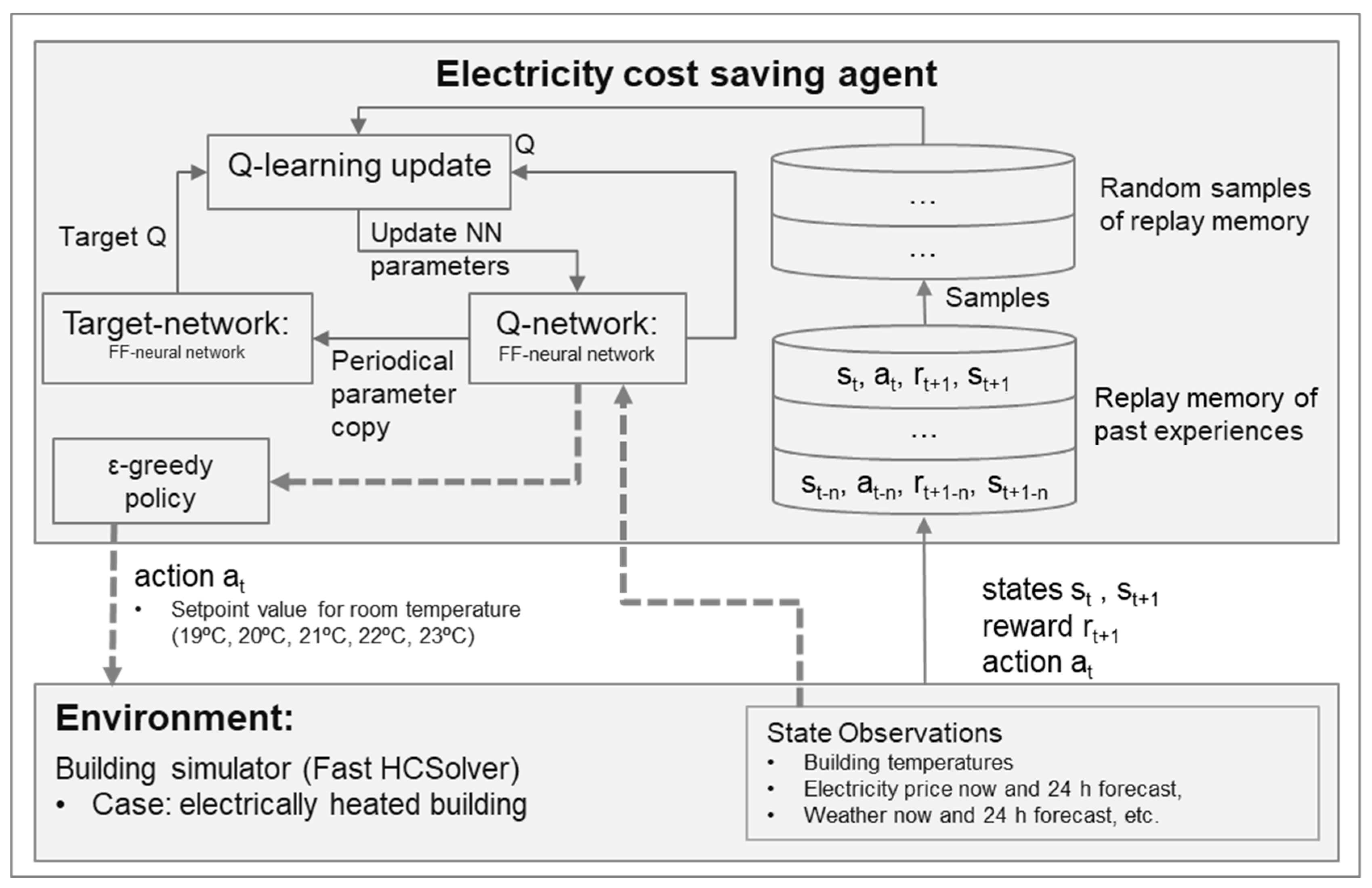
2.2. Implementation of the Algorithm

The implemented reinforcement learning case for finding the best next hour electric heating setpoint values for achieving optimal reward (electricity bill savings) is shown in Figure 2.

In this case, the environment is the building, heating system, and the surrounding world. To measure the state of the environment, we chose observations that could be easily measured also from real buildings. This includes:

• timestamp (hour of day and day of week);
• weather (outdoor temperature, global radiation, and diffuse radiation) current value and forecast for next 24 h;
• electricity price and its forecast for the next 24 h;
• and temperature measurements from the building.

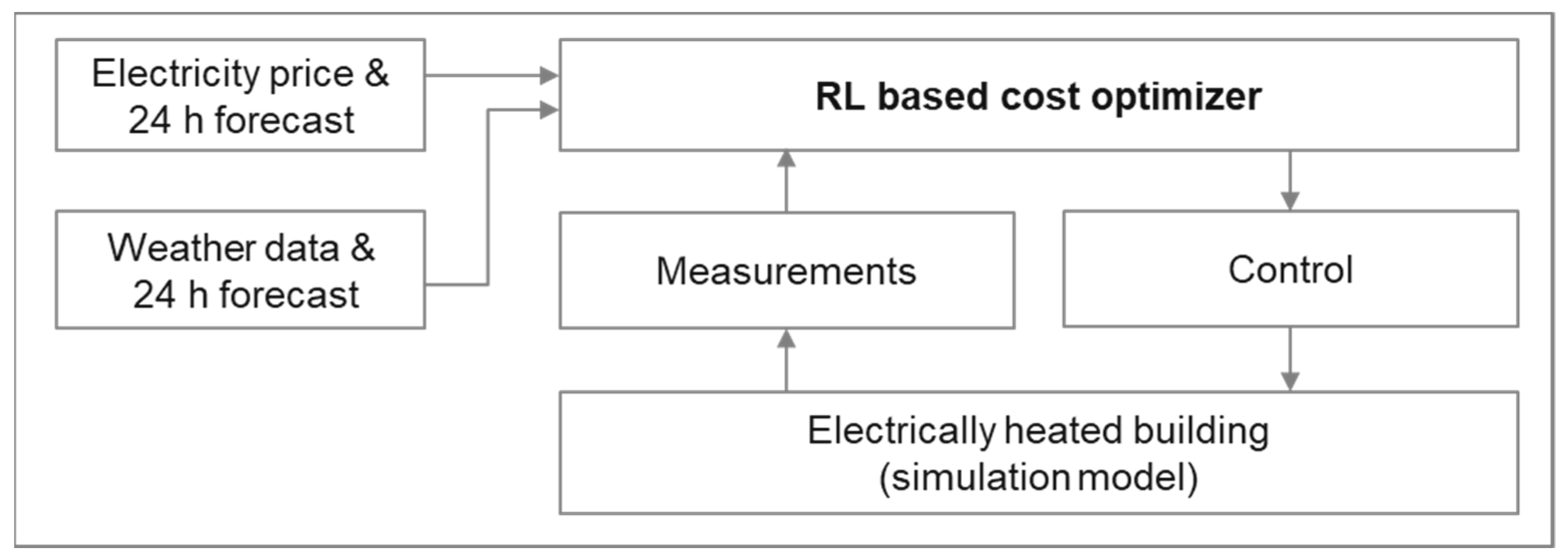
The agent, here the heating setpoint controller, is trying to minimize the electricity bill by changing the indoor temperature setpoint hour by hour. It has five different options for valid actions: set points between 19 °C and 23 °C.

In this study, the reward function is constructed based on the two objectives: minimizing the cost from electricity usage and retaining thermal comfort. The first part is formed as the negation of the electricity cost calculated from the hourly electricity price and simulated heating energy consumption. Thermal comfort is a more complex measure to value. Here, the occupants are assumed to prefer indoor temperatures higher than 21 °C. Therefore, the situations where the measured indoor temperature gets lower than 21 °C are punished with a correction factor relative to the difference from the desired temperature. The values near 21 °C should also be preferred to the lower ones, since then the setpoint is still adjustable in case an even higher electricity price occurs. However, it is assumed that the penalty is only needed when the indoor temperature is less than 21 °C since the elevated temperatures are already less desirable through increasing heat consumption. Three different reward functions are tested: reward based only on the electricity cost (Equation (2)), reward with linear penalty from temperature difference (Equation (3)), and reward with a second-order penalty (Equation (4)):

$$R_{t+1}=-\left(p\ast E\right),$$

(2)

$$R_{t+1}=\{\begin{array}{c}-\left(p\ast E\right)\ast \left(1+\beta \ast \left(21-T_{indoor}\right)\right),if T_{indoor}<21\\ -\left(p\ast E\right),otherwise\end{array},$$

(3)

$$R_{t+1}=\{\begin{array}{c}-\left(p\ast E\right)\ast \left(1+\beta \ast {\left(21-T_{indoor}\right)}^2\right),if T_{indoor}<21\\ -\left(p\ast E\right),otherwise\end{array},$$

(4)

where T_indoor is the measured indoor temperature, E is the heating energy consumption, β is a coefficient to weight the penalty, and p is the electricity price.

The value of the Q function and target Q are approximated with two identical neural networks. A feed forward net with four hidden layers and 256 neurons is used. The observations are normalized with a minmax scaler. Algorithms are implemented with Java utilizing the deeplearning4j [40] library for calculation of the neural networks.

2.3. Environment

The environment consists of three parts: building simulator, weather measurements, and electricity price information. The building is simulated with a FastHC building simulator. The FastHC building simulator model is based on an equivalent resistance-capacitance (R-C) model, including five resistances, five nodes, and one capacitance. The used R-C model is documented in more detail in EN ISO 13790:2008 standard [41]. The model also includes methods for calculating energy losses due to ventilation and infiltration in buildings (EN 15241:2007 [42]) and methods for calculating solar radiation. In addition, the FastHC Solver simulator environment can utilize a default value database, which includes typical values for several types of buildings built in different decades. The simulations are run with a one-hour timestep.

For simulations and algorithm input, the weather measurements of Helsinki provided by the Finnish Meteorological Institute’s open data service [43] are utilized. The dataset contains values for outside temperature, as well as global and diffuse radiation, with one hour sampling time.

Many energy companies in Finland offer contracts that are based on the spot prices of electricity in Nord Pool. The price in Nord Pool is fluctuating hour by hour and day-ahead prices are published each day in the afternoon [6]. In the simulations, the spot price history from ENTSOE platform [44] is used. In real cases, the price per used kWh would be higher for the end user than just the spot price, due to taxes and energy company margins. Before 2021, the electricity price was cheap and stable, but during the last year, it became radically more expensive and fluctuating than before (

Table 1. Mean, minimum, maximum, and standard deviation of electricity price by year (€/MWh).

	2019	2020	2021	2022 (Until 11 September)
mean	44.0	28.0	72.3	139.7
min	0.1	−1.7	−1.4	−1.0
max	200.0	254.4	1000.1	861.1
std	15.3	21.1	66.0	126.1

).

2.4. Buildings and Performance Tests

The buildings considered here are single-family buildings with direct electricity heating and no cooling devices. All simulated buildings have a floor area of 120 m². However, the building parameters, such as U-values and share of windows, are configured to represent typical Finnish building for certain time range. Following buildings are calculated:

• typical building of years 2011–2017;
• typical building of years 2001–2010;
• typical building of years 1991–2000;
• typical building of years 1981–1990;
• typical building of years 1971–1980;
• and typical building of years 1961–1970.

For each building, two reference cases with static indoor temperature setpoints are simulated, 21 °C as baseline and 19 °C as the easiest way to obtain cost savings, but at the expense of reduced thermal comfort. These are compared to the heating cost and indoor temperature resulting from the use of RL. The time range from 1 January 2019 to 9 September 2022 is considered.

A building model representing buildings constructed between 2001 and 2010 is used for configuring the method and searching proper parameters. The rest of the buildings are tested with the same parameter set.

3. Results

3.1. Comparison of Different Reward Functions

Selecting the right reward function is crucial for indoor comfort. If the penalty from too low indoor temperature is linear (Equation (3)) instead of second-order (Equation (4)), then the indoor temperature is shifting closer to 19 °C (Figure 3). Respectively, in case the penalty is totally ignored (Equation (2)), the indoor temperature nearly reaches 19 °C (Figure 4). The thermal conditions are clearly most desired in case of second-order penalty (Figure 5).

The penalty function has a little less effect on the electricity costs (

Table 2. Cost savings of building constructed between 2001 and 2010 for different reward functions.

	2019	2020	2021	2022 (Until 11 September)
no penalty	12%	17%	13%	21%
linear penalty	11%	23%	17%	27%
second-order penalty	−2%	8%	13%	27%

). In cases where the temperature is all the time near the lower limit, there is less reserve to be used, when the algorithm really would need to reduce electricity usage. With the second-order penalty, the indoor temperature is kept higher than with the linear penalty, and thus also the energy usage and further energy cost is higher, especially in cases with less variable energy price. However, both reward functions reach the same level in savings during the year 2022. For the rest of the calculations, the second-order penalty (Equation (4)) is selected.

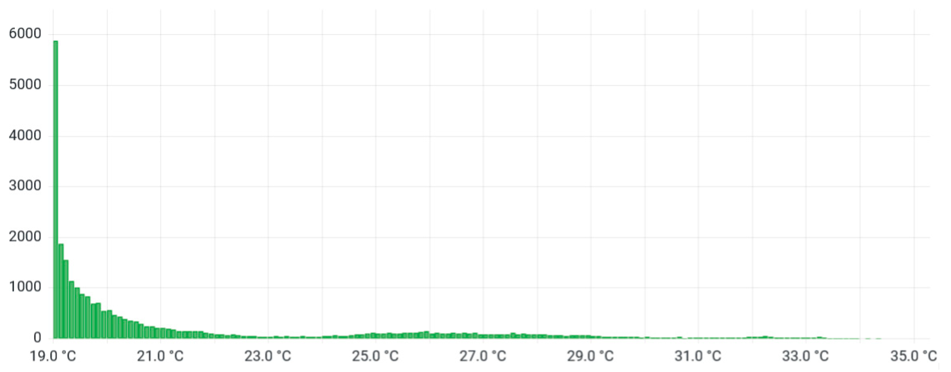
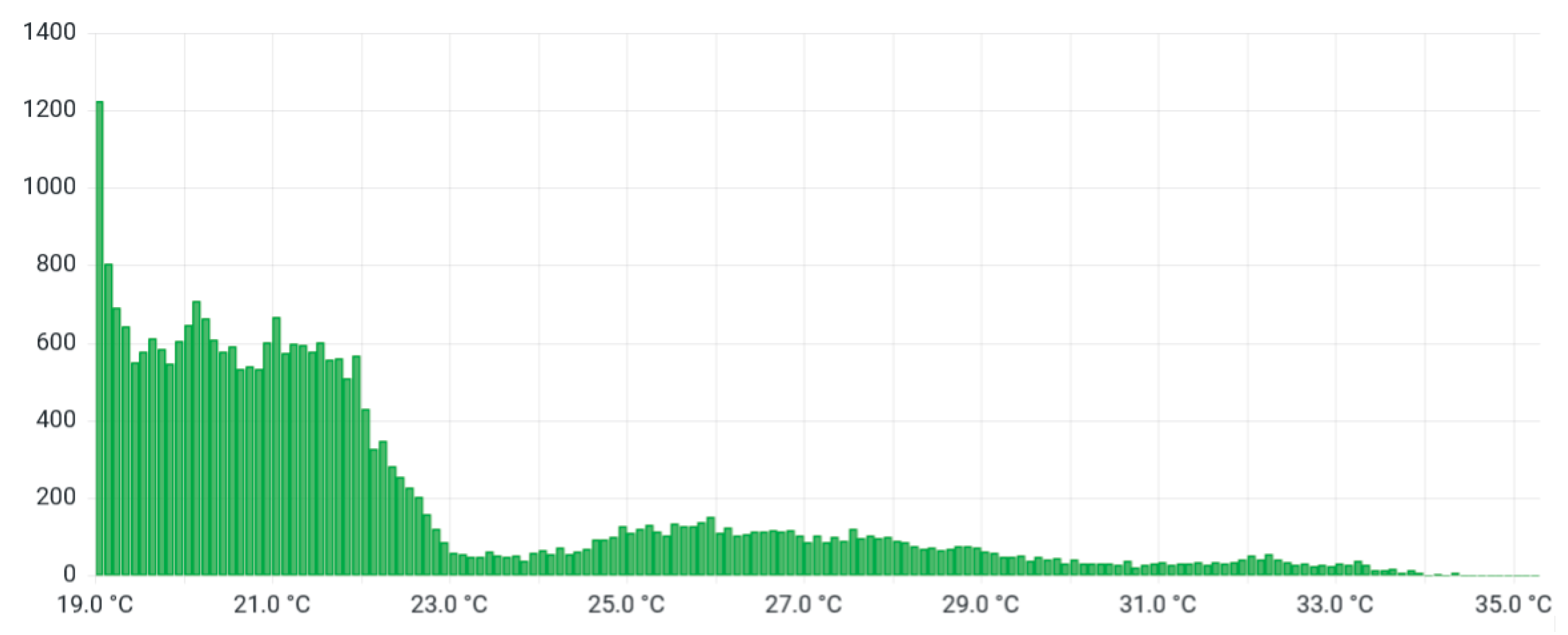
3.2. Indoor Temperature for Different Buildings

The average indoor temperature and standard deviation from the simulations utilizing varying set points calculated with RL is presented in

Table 3. Average indoor temperature and standard deviation of October–March in simulations utilizing RL.

Building Construction Year	avg (Tindoor)	std (Tindoor)
1961–1970	21.1 °C	0.79
1971–1980	21.0 °C	0.78
1981–1990	20.8 °C	0.91
1991–2000	20.8 °C	0.84
2001–2010	20.8 °C	0.89
2011–2017	20.6 °C	0.83

. Just the heating season (from October to end of March) is considered in calculation of these values to prevent distortion from summertime temperature rise. The average temperature for all RL cases is near 21 °C, which is considered as the pursued temperature.

Example of the share of different temperatures is presented in the indoor temperature histogram (Figure 5). The temperature is balancing around the desired value instead of drifting to lower values. There is no cooling in the simulated buildings, which results in the high summertime temperatures that can be seen in the histograms as well.

3.3. Cost Savings by Simulation Year

The electricity cost is calculated from the simulated heating electricity consumption and electricity price. The average cost savings of the buildings for each simulation year are presented in

Table 4. Average cost savings from the baseline (21 °C) per simulation year.

	2019	2020	2021	2022 (Until 11 September)
19 set point	15%	18%	12%	19%
RL	−1%	8%	10%	23%

, and an example of the cumulative cost for each year is shown in Figure 6. From the results, it can be seen that in the years 2019 and 2020, the stable 19 °C setpoint is outperformed the current RL agent. During this time range, the electricity price was low and stable; also, at the beginning of 2019, the algorithm started learning from scratch.

By the end of year 2021 the RL had nearly reached the same level, and during year 2022, it even obtained higher savings than the low set point option, even though the year 2022 is still ongoing. During the year 2022 and at the end of 2021 the electricity price was fluctuating significantly and reached many times higher peak values than before, so delaying heating with one hour can have a major impact to the total electricity bill.

3.4. Cost Savings of Buildings Based on Construction Year

Comparing the savings based on construction year (

Table 5. Average annual cost (€) of space heating electricity with stable 21 °C set point and savings (%) with different temperature setpoints.

Building Construction Year	sp 21 (€)	sp 19 (%)	RL (%)
1961–1970	1619	15%	6%
1971–1980	1523	15%	7%
1981–1990	905	16%	15%
1991–2000	920	15%	12%
2001–2010	874	16%	14%
2011–2017	451	16%	17%

), it seems that the percentual savings are better the less the building is consuming electricity. Compared to the stable 19 °C, savings with the oldest buildings are lesser. However, also with these buildings during the last simulation year, the difference decreased significantly.

3.5. Energy Savings by Simulation Year

The delivered heating electricity is affecting the reward only through the payments, and thus it is not significantly reduced with the current algorithm. Average energy savings of each simulation year are presented in

Table 6. Average energy savings from the baseline (21 °C) of the buildings per simulation year.

	2019	2020	2021	2022 (Until 11 September)
19 set point	16%	19%	15%	19%
RL	−1%	1%	2%	4%

.

4. Conclusions

This paper proposes a reinforcement learning-based electricity cost saving method that increases the heating of an electrically heated building when electricity is cheap and reduces the electricity use when it is expensive, in such a way that the resident does not notice it as thermally uncomfortable.

The results indicate that it is possible to lower heating costs significantly with RL. Depending on the fluctuations of the electricity price, the savings can reach the same level as when reducing the stable indoor temperature setpoint by two degrees, or be even higher. In this study, the algorithm was less successful during the first two years, and performing a lot better during the years 2021 and 2022. First, in the beginning of the year 2019, the agent started training the deep neural networks from scratch, and as experience was gained, the operation began improving. Second, the electricity price level and variability from the end of 2021 onwards is radically different from the first simulation years. This results in higher savings from optimizing the heating times.

Here, it is assumed that the occupants prefer indoor temperatures closer to 21 °C, but in real cases, the end users might also suffer from temperature changes. Transitions in the temperature should be rather small and slow to keep user experience positive. Presumably, the lags in the heating system and heat capacity of the building and furnishing are supporting here, but this would require further analysis, e.g., by integrating thermal sensation calculations with the human thermal model [45] to the simulations.

The agent is not aimed to minimize the total delivered electricity, and consequently, the consumed electricity is just slightly less than with the 21 °C reference case, and with the stable 19 °C indoor temperature higher, energy saving could be reached. However, the electricity price is also dependent on the production type. Usually, the price is lower when the share of renewable energy, e.g., from wind power, is high. Thus, it would be interesting to include some estimate of the emissions based on the production types.

Selecting the right reward function has a high impact on the results. By changing it, the algorithm can focus on different targets, e.g., energy savings or minimizing emissions. However, it must balance between the savings and thermal indoor comfort, not only to keep residents contented, but also to be able to utilize the heat capacity of the building and retain the controllability of indoor temperature.

For the future work, approaches for fine-tuning the energy cost saving agent for more complex building energy systems should be investigated, e.g., by taking also hot water boilers, heat pumps, local energy production, such as PV panels, and energy storages into account.

In addition, the presented method is tested with building simulation models, which represent typical Finnish one-family house constructed between 1961 and 1970, 1971 and 1980, 1981 and 1990, 1991 and 2000, 2001 and 2010, and 2011 and 2017. Based on these tests, the energy cost saving agent can be scaled for different Finnish one-family houses. However, the tested method does have higher performance with newer buildings. The oldest buildings have typically less insulation and a lack of heat recovery systems. This means that they have faster reaction to heating power reductions, which results in a less dynamical margin for the indoor temperature control. However, it is important to note that the RL parameters are calibrated with 2001–2010 building, and it is not tested how the much older buildings would behave with variant configuration. Furthermore, for the future work, testing with different types of buildings in various climatic conditions should be performed.

From a practical deployment point of view, the system has several challenges in the future. The first challenge is related to the initialization of the agent. More specifically, in real cases, the controller cannot behave randomly for a long time, so it should be studied if the algorithm can adapt to a new building fast enough, or should the agent be pretrained with a simulator beforehand. Furthermore, after major renovations, the system should be able to readjust to the new consumption and be able to forget the old behavior in descent time.

The second challenge is related to the fact that many buildings do not have an existing building automation and controller system (BACS) or IoT connected room temperature controller or smart thermostats and related secure REST API for daily communication with a cloud-based electricity cost saving agent. This means the integration of the presented approach to real use would require some physical installations to be performed.

Overall, scaling this kind of a solution could increase the flexibility in the electricity market, which is important also from the electricity network balance and related electricity price point of view.

References

1. European Commission. A Clean Planet for All: A European Strategic Long-Term Vision for a Prosperous, Modern, Competitive and Climate Neutral Economy. Communication From the Commission 2018. Available online: https://www.europeansources.info/record/communication-a-clean-planet-for-all-a-european-strategic-long-term-vision-for-a-prosperous-modern-competitive-and-climate-neutral-economy/ (accessed on 21 December 2022).
2. An European Green Deal. Available online: https://commission.europa.eu/strategy-and-policy/priorities-2019-2024/european-green-deal_en (accessed on 16 January 2023).
3. Nejat, P.; Jomehzadeh, F.; Taheri, M.M.; Gohari, M.; Majid, M.Z.A. A Global Review of Energy Consumption, CO 2 Emissions and Policy in the Residential Sector (with an Overview of the Top Ten CO2 Emitting Countries). Renew. Sustain. Energy Rev. 2015, 43, 843–862. [Google Scholar] [CrossRef]
4. European Commission Directorate—General for Energy. Comprehensive Study of Building Energy Renovation Activities and the Uptake of Nearly Zero-Energy Buildings in the EU: Final Report; Publications Office of the EU: Geneva, Switzerland, 2019. [Google Scholar]
5. European Commission; Centre, J.R.; Tsiropoulos, I.; Nijs, W.; Tarvydas, D.; Ruiz, P. Towards Net-Zero Emissions in the EU Energy System by 2050: Insights from Scenarios in Line with the 2030 and 2050 Ambitions of the European Green Deal; Publications Office of the EU: Geneva, Switzerland, 2020. [Google Scholar]
6. Nord Pool. Available online: https://www.nordpoolgroup.com/ (accessed on 12 January 2023).
7. Knapik, O. Modeling and Forecasting Electricity Price Jumps in the Nord Pool Power Market; CREATES Research Paper 2017-7; Department of Economics and Business Economics, Aarhus University: Aarhus, Danmark, 2017. [Google Scholar]
8. Alimohammadisagvand, B.; Alam, S.; Ali, M.; Degefa, M.; Jokisalo, J.; Sirén, K. Influence of Energy Demand Response Actions on Thermal Comfort and Energy Cost in Electrically Heated Residential Houses. Indoor Built Environ. 2017, 26, 298–316. [Google Scholar] [CrossRef]
9. Behl, M.; Jain, A.; Mangharam, R. Data-Driven Modeling, Control and Tools for Cyber-Physical Energy Systems. In Proceedings of the 2016 ACM/IEEE 7th International Conference on Cyber-Physical Systems (ICCPS), Vienna, Austria, 11–14 April 2016; pp. 1–10. [Google Scholar]
10. Péan, T.Q.; Salom, J.; Costa-Castelló, R. Review of Control Strategies for Improving the Energy Flexibility Provided by Heat Pump Systems in Buildings. J. Process Control 2019, 74, 35–49. [Google Scholar] [CrossRef]
11. Avci, M.; Erkoc, M.; Rahmani, A.; Asfour, S. Model Predictive HVAC Load Control in Buildings Using Real-Time Electricity Pricing. Energy Build 2013, 60, 199–209. [Google Scholar] [CrossRef]
12. Li, X.; Malkawi, A. Multi-Objective Optimization for Thermal Mass Model Predictive Control in Small and Medium Size Commercial Buildings under Summer Weather Conditions. Energy 2016, 112, 1194–1206. [Google Scholar] [CrossRef]
13. Zhang, H.; Seal, S.; Wu, D.; Bouffard, F.; Boulet, B. Building Energy Management with Reinforcement Learning and Model Predictive Control: A Survey. IEEE Access 2022, 10, 27853–27862. [Google Scholar] [CrossRef]
14. Fischer, D.; Bernhardt, J.; Madani, H.; Wittwer, C. Comparison of Control Approaches for Variable Speed Air Source Heat Pumps Considering Time Variable Electricity Prices and PV. Appl. Energy 2017, 204, 93–105. [Google Scholar] [CrossRef]
15. Vandermeulen, A.; Vandeplas, L.; Patteeuw, D.; Sourbron, M.; Helsen, L. Flexibility Offered by Residential Floor Heating in a Smart Grid Context: The Role of Heat Pumps and Renewable Energy Sources in Optimization towards Different Objectives. In Proceedings of the IEA Heat Pump Conference, Rotterdam, The Netherlands, 15–18 May 2017. [Google Scholar]
16. Ala’raj, M.; Radi, M.; Abbod, M.F.; Majdalawieh, M.; Parodi, M. Data-Driven Based HVAC Optimisation Approaches: A Systematic Literature Review. J. Build. Eng. 2022, 46, 103678. [Google Scholar] [CrossRef]
17. Liu, T.; Xu, C.; Guo, Y.; Chen, H. A Novel Deep Reinforcement Learning Based Methodology for Short-Term HVAC System Energy Consumption Prediction. Int. J. Refrig. 2019, 107, 39–51. [Google Scholar] [CrossRef]
18. Raza, R.; Hassan, N.U.; Yuen, C. Determination of Consumer Behavior Based Energy Wastage Using IoT and Machine Learning. Energy Build 2020, 220, 110060. [Google Scholar] [CrossRef]
19. Esrafilian-Najafabadi, M.; Haghighat, F. Impact of Occupancy Prediction Models on Building HVAC Control System Performance: Application of Machine Learning Techniques. Energy Build 2022, 257, 111808. [Google Scholar] [CrossRef]
20. Chaudhuri, T.; Soh, Y.C.; Li, H.; Xie, L. Machine Learning Based Prediction of Thermal Comfort in Buildings of Equatorial Singapore. In Proceedings of the 2017 IEEE International Conference on Smart Grid and Smart Cities (ICSGSC), Singapore, 23–26 July 2017; pp. 72–77. [Google Scholar]
21. Kusiak, A.; Tang, F.; Xu, G. Multi-Objective Optimization of HVAC System with an Evolutionary Computation Algorithm. Energy 2011, 36, 2440–2449. [Google Scholar] [CrossRef]
22. Nassif, N. Modeling and Optimization of HVAC Systems Using Artificial Neural Network and Genetic Algorithm. Build Simul. 2014, 7, 237–245. [Google Scholar] [CrossRef]
23. Amin, U.; Hossain, M.J.; Fernandez, E. Optimal Price Based Control of HVAC Systems in Multizone Office Buildings for Demand Response. J. Clean Prod. 2020, 270, 122059. [Google Scholar] [CrossRef]
24. Yuan, X.; Pan, Y.; Yang, J.; Wang, W.; Huang, Z. Study on the Application of Reinforcement Learning in the Operation Optimization of HVAC System. Build Simul. 2021, 14, 75–87. [Google Scholar] [CrossRef]
25. Fazenda, P.; Veeramachaneni, K.; Lima, P.; O’Reilly, U.-M. Using Reinforcement Learning to Optimize Occupant Comfort and Energy Usage in HVAC Systems. J. Ambient. Intell. Smart Environ. 2014, 6, 675–690. [Google Scholar] [CrossRef]
26. Liu, S.; Henze, G.P. Experimental Analysis of Simulated Reinforcement Learning Control for Active and Passive Building Thermal Storage Inventory: Part 1. Theoretical Foundation. Energy Build 2006, 38, 142–147. [Google Scholar] [CrossRef]
27. Barrett Enda and Linder, S. Autonomous HVAC Control, A Reinforcement Learning Approach. In Proceedings of the Machine Learning and Knowledge Discovery in Databases: European Conference, ECML PKDD 2015, Porto, Portugal, 7–11 September 2015; Springer International Publishing: Cham, Germany, 2015; pp. 3–19. [Google Scholar]
28. Costanzo, G.T.; Iacovella, S.; Ruelens, F.; Leurs, T.; Claessens, B.J. Experimental Analysis of Data-Driven Control for a Building Heating System. Sustain. Energy Grids Netw. 2016, 6, 81–90. [Google Scholar] [CrossRef]
29. Ruelens, F.; Iacovella, S.; Claessens, B.; Belmans, R. Learning Agent for a Heat-Pump Thermostat with a Set-Back Strategy Using Model-Free Reinforcement Learning. Energy 2015, 8, 8300–8318. [Google Scholar] [CrossRef]
30. Li, B.; Xia, L. A Multi-Grid Reinforcement Learning Method for Energy Conservation and Comfort of HVAC in Buildings. In Proceedings of the 2015 IEEE International Conference on Automation Science and Engineering (CASE), Gothenburg, Swede, 24–28 August 2015; pp. 444–449. [Google Scholar]
31. Wei, T.; Wang, Y.; Zhu, Q. Deep Reinforcement Learning for Building HVAC Control. In Proceedings of the 54th Annual Design Automation Conference 2017, Austin, TX, USA, 18–22 June 2017; pp. 1–6. [Google Scholar] [CrossRef]
32. Azuatalam, D.; Lee, W.-L.; de Nijs, F.; Liebman, A. Reinforcement Learning for Whole-Building HVAC Control and Demand Response. Energy AI 2020, 2, 100020. [Google Scholar] [CrossRef]
33. Biswas, D. Reinforcement Learning Based HVAC Optimization in Factories. In Proceedings of the Eleventh ACM International Conference on Future Energy Systems, Online, 22–26 June 2020; pp. 428–433. [Google Scholar]
34. Gupta, A.; Badr, Y.; Negahban, A.; Qiu, R.G. Energy-Efficient Heating Control for Smart Buildings with Deep Reinforcement Learning. J. Build. Eng. 2021, 34, 101739. [Google Scholar] [CrossRef]
35. Sutton, R.S.; Barto, A.G. Reinforcement Learning: An Introduction, 2nd ed.; MIT Press: Cambridge, MA, USA, 2018. [Google Scholar]
36. Watkins, C.J.C.H. Learning from Delayed Rewards; King’s College: Cambridge, UK, 1989. [Google Scholar]
37. van Hasselt, H.; Guez, A.; Silver, D. Deep Reinforcement Learning with Double Q-Learning. In Proceedings of the Thirtieth AAAI Conference on Artificial Intelligence, Phoenix, AZ, USA, 13–17 February 2016; p. 30. [Google Scholar] [CrossRef]
38. Mnih, V.; Kavukcuoglu, K.; Silver, D.; Rusu, A.A.; Veness, J.; Bellemare, M.G.; Graves, A.; Riedmiller, M.; Fidjeland, A.K.; Ostrovski, G.; et al. Human-Level Control through Deep Reinforcement Learning. Nature 2015, 518, 529–533. [Google Scholar] [CrossRef] [PubMed]
39. Brunton, S.L.; Kutz, J.N. Data-Driven Science and Engineering; Cambridge University Press: Cambridge, MA, USA, 2022; ISBN 9781009089517. [Google Scholar]
40. Deeplearning4j Suite Overview—Deeplearning4j. Available online: https://deeplearning4j.konduit.ai/ (accessed on 12 January 2023).
41. ISO—ISO 13790:2008; Energy Performance of Buildings—Calculation of Energy Use for Space Heating and Cooling. Available online: https://www.iso.org/standard/41974.html (accessed on 12 January 2023).
42. EN 15241:2007; Ventilation for Buildings—Calculation Methods for Energy Losses Due to Ventilation. Available online: https://standards.iteh.ai/catalog/standards/cen/4138127b-0434-4265-95ef-4b075788e878/en-15241-2007 (accessed on 9 May 2022).
43. Open Data—Finnish Meteorological Institute. Available online: https://en.ilmatieteenlaitos.fi/open-data (accessed on 12 January 2023).
44. ENTSO-E Transparency Platform. Available online: https://transparency.entsoe.eu/ (accessed on 12 January 2023).
45. Holopainen, R. A Human Thermal Model for Improved Thermal Comfort; School of Engineering, Aalto University: Espoo, Finland, 2012. [Google Scholar]
Figure 1. System model for optimizing building electricity cost.
Buildings 13 00427 g001
Figure 2. The implemented reinforcement learning case for finding the best next day electric heating setpoint values for achieving optimal reward (electricity bill savings).
Buildings 13 00427 g002
Figure 3. Indoor temperature histogram for a 2001–2010 building with linear penalty.
Buildings 13 00427 g003
Figure 4. Indoor temperature histogram for a 2001–2010 building, when there is no penalty from too low indoor temperature.
Buildings 13 00427 g004
Figure 5. Indoor temperature histogram for a 2001–2010 building, with second-order penalty.
Buildings 13 00427 g005
Figure 6. Cumulative energy cost for each simulation year for a 2001–2010 building.
Buildings 13 00427 g006