Abstract
Detecting and measuring cracks during laboratory experiments to characterize material behavior is an important task in building materials research. In this context, the evaluation of crack distribution is emphasized, including crack widths. Contact-free, optical 2D/3D-measuring Digital Image Correlation systems are used to analyze the full-field deformation of the surface. To examine the parameters affecting crack analysis through this measurement mode, a parameter study was conducted analyzing carbon textile-reinforced concrete tensile strength tests. For this purpose, facet size, facet overlap, and the threshold for crack identification based on major strain calculations in the evaluation were varied. The novelty lies in the in-depth exploration of these parameters to enhance crack analysis accuracy. To facilitate this, an automated crack evaluation tool (ACE) was developed and validated through tensile tests. The results of this paper provide evidence of the key parameters that influence crack analysis in textile reinforced concrete and contribute valuable guidance on optimum setting parameters.
1. Introduction
In the field of reinforced concrete buildings, damage mechanisms like cracks can occur. In this context, crack analysis is typically one of the most common indicators of damage [1,2]. Therefore, it is crucial to detect and measure cracks, even in laboratory experiments for material behavior characterization. The building materials research focuses on the evaluation of crack distribution, with particular attention paid to the crack width [3,4]. Deformation measurement devices like linear variable differential transformers (LVDT) or displacement transducers are commonly used to monitor crack widths, and are well-established techniques [3]. However, these devices prove to be inadequate for precisely analyzing multiple and fine crack patterns within textile reinforced concrete (TRC) [3,5]. Textile reinforced concrete (TRC) is primarily known for its lightness, durability and high load-bearing capacity in comparison to conventional reinforcement materials. Suitable for the repair of building surfaces, TRC enables limited deformation and a distribution of multiple cracks, resulting in a reduced crack width due to its larger surface area and enhanced bond strength. In this context, an alternative method for crack measurement can be implemented by employing camera imaging on the specimen surface and capturing image sequences during load tests. These contact-free, time-resolved techniques enable numerous advantages for crack analysis such as multidimensional, full-field data evaluation [6].
To provide an overview of crack evaluation methodologies, different methods for example image-based crack detection, Laser Doppler Vibrometer measurements and Digital Image Correlation analysis are presented [6,7,8]. Three-dimensional Laser Vibrometry systems based on the Doppler effect are employed as non-contact measurement systems [9]. Longo et al. [10] introduced a crack detection method of Surface Acoustic Waves with Laser Doppler Vibrometer using reflections.
Digital Image Correlation analysis can be summarized into the category of methodological for extracting cracks from the concrete surface in images [6,11]. Edge detection techniques employ algorithm operators such as Sobel or Laplace to identify cracks as an edge in an image under suitable illumination. However, this approach has limitations, as it can only detect cracks with a width of one pixel or more. Applying this method, Nyathi et al. [1] developed an approach for measuring crack width in millimeters using image processing algorithms in conjunction with a unique laser beam technique. A further example of this methodology is given by Sohn et al. [12]. To investigate the algorithms, Kim et al. [13] conducted a comparative analysis of image binarization methods for crack identification in structural cracks. Moreover, Wang et al. [14] summarized four categories of crack detection algorithms: integrated algorithms, morphological approaches, percolation-based image processing and practical techniques.
The second category involves employing targets affixed to the measurement surface to establish 3D coordinates [6]. This measurement can be performed using commercially available systems. As an example, Barazzetti et al. [15] conducted studies demonstrating crack width measurements using discrete targets attached to concrete specimens.
A target-free, full-field subpixel-accurate measurement technique can be achieved through the application of image matching techniques, which leverage artificial surface texture to identify homologous points in consecutive images within an image sequence [6]. This technique, known as Digital Image Correlation (DIC), was developed in the early 1980s and has been extensively applied in laboratory experiments, particularly for crack analysis in TRC [3,16]. The resulting capabilities for the continuous monitoring of deformation, crack, and damage development on object surfaces represent a significant enhancement in the quality of experimental investigations in civil engineering. Building upon this, Hampel et al. [6] developed a cascaded image analysis approach that identifies discontinuities in surface deformation vector fields. These deformation vector fields were generated through successive stereo image captures using cross-correlation or least-square matching. The measurement can be performed using commercially available systems.
After the DIC measurements, the data were analyzed manually via different approaches in the DIC software using images from the various deformation stages. The first method involves extracting local deformation data using a virtual extensometer manually positioned at the center of the specimen in the DIC software [16,17]. These data are then used to determine the numbers and widths of cracks, following the methodologies of Ohno et al. [18]. In this approach, each peak observed on the local deformation curve is identified as a crack, and its width is calculated. In this case, the crack width is evaluated at the level of the manually set virtual extensometer, depicted Figure 1. Further studies such as those by Zhu et al. [19] and Godek et al. [16] used this evaluation method.
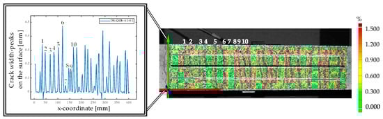
Figure 1.
Manual crack width evaluation of the local deformation in the DIC software adapted by [16,18].
Besides the described method, an additional evaluation process in the DIC software has been conducted manually by visualizing the major strain component εmax on the surface. The analysis of crack width is performed perpendicular to the tensile loading direction [3]. The method for calculating major strain is shown in Equations (1)–(4) and Figure 2 [20]:
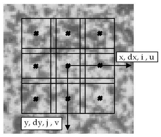
Figure 2.
Schematic visualization of the calculation with i and j as facet unit coordinates, u and v representing horizontal and vertical displacements of the facet center, and dx and dy indicating the distance between the facet center in the reference image adapted from [20].
The crack width was determined based on three virtual extensometers on the surface for CTRC tensile test specimens [3]. This process involved the manual placement of facet points along the crack boarders and the selection of the scaling factor, as shown in Figure 3. The scaling factor determines the visualization of the crack width, and facet points are manually placed at the color transition of the crack boarder.
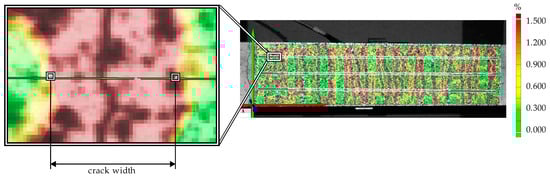
Figure 3.
Manual crack width evaluation in the DIC software adapted by [3].
Subsequently, the software calculated the deformation parallel to the direction of tensile loading for each deformation stage in the three manually set extensometers. Exemplarily, the major strain scaling factor was set to 1.5% for CTRC crack distribution by [3] and 10% for fiber concrete tests testing by Domski et al. [21].
The presented evaluation methods can be used for analyzing measurements in the field of laboratory investigation in materials research. Both methods can determine crack widths based on the major strain measured by the DIC system. However, a disadvantage lies in the manual placement of extensometers. Manually, only selected positions are evaluated, and the average crack width across the entire specimen is not determined. The creation of an extensometer across the entire specimen can only be realized with a considerable amount of time.
In addition to the crack analysis, parameters such as pattern visibility, lighting effects, aperture, number of cameras, exposure time and exposure type affect the crack evaluation [3,11,22,23]. To quantify the impact of camera resolution on mechanical properties and multiple crack characteristics using DIC, Godek et al. [16] conducted experiments on cementitious composites. This research demonstrated that increased resolution results in finer pattern precision and led to a twofold increase in the number of detected cracks during the analysis. During the evaluation process of measurements using DIC, key parameters for evaluation include facet size, the quantity of images per measurement, the spacing between two facets (facet overlap), strain tensors’ neighborhood, averaging spatially and temporally, and the threshold for the scaling factor based on the major strain [3,22]. However, it should be noted that the accuracy of image analysis is constrained by systematic and random errors. Systematic errors may arise from deficiencies in the mathematical model or mechanical instabilities in the camera setup, such as temperature-induced deformation or mechanical instabilities. On the other hand, random errors can result from factors like image noise, rounding errors in floating point calculations, mechanical instabilities, and over-determination errors in the multi-camera setups [22].
In order to guide the setting of optimum parameters influencing crack analysis based on Digital Image Correlation, a parameter study was conducted using carbon textile reinforced concrete (CTRC) tensile strength tests. This paper examined facet sizes from 11 × 11 pixels to 23 × 23 pixels, facet overlap from 1 to 7 pixels and the scaling factor for crack identification based on the major strain calculation. To facilitate this, an automated crack evaluation tool (ACE) was developed and validated through tensile tests.
2. Materials
In this study, a textile reinforced composite composed of a commercial carbon textile reinforcement and two repair mortars, according to TR-IH [24,25], were used for the evaluation. The carbon textile reinforcement, referred to as CTR-EP-Sand, was impregnated with epoxy-resin and additionally surface modified. The surface modification involved a subsequent coating of epoxy-resin and quartz sand. The CTR-EP-Sand is shown in the following Figure 4, and the material parameters are summarized in Table 1.
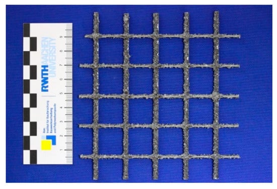
Figure 4.
Investigated carbon textile reinforcement CTR-EP-Sand.

Table 1.
Material parameters of the carbon textile reinforcement according to the manufacturer’s specification [26].
The repair mortars were polymer-modified cement-based mortars designed for the retrofitting of the concrete surface with a maximum grain size of 2 mm. According to the manufacturer’s specification, the mortars differed in terms of the intended method of application. RM-A4 is a repair mortar applied by hand, while SRM-A4 is applied by wet spraying [24,25]. The material properties of the mortars are summarized in Table 2.
Table 2.
Material parameters of the repair mortars.
3. Methods
To investigate the parameter setting for evaluating the crack distribution of TRC, two steps were followed. First, an automated crack evaluation tool (ACE) for measurements using DIC was developed. The ACE was designed based on results of laboratory experiments using an optical 2D/3D-measuring system ARAMIS® with CTR-EP-Sand and RM-A4 and validated based on a manual crack width evaluation method within the DIC software, shown in Figure 3. With ACE, the setting parameters for the evaluation process were modified and analyzed with the objective to evaluate a realistic crack distribution. Therefore, the scaling factor for determining crack width depending on the major strain and the adjustable facet size and facet overlap were examined in a parameter study on specific crack width in tensile strength tests. The laboratory experiments were conducted on the material combination CTR-EP-Sand and RM-A4, referred to as RM, and CTR-EP-Sand and SRM-A4, referred to as SRM. For each batch, two tests were conducted. Table 3 gives an overview of the test and validation series.
Table 3.
Overview of the test and validation series.
3.1. Experimental Setup and Testing Procedure
3.1.1. Tensile Strength Test on CTRC
To determine the crack distribution for the parameter study, tensile strength tests were conducted on rectangular CTRC specimens, depicted in Figure 5. The specimen dimensions for RM were 1000 × 100 × 20 (L × W × T) in mm, and for SRM 500 × 60 × 20 (L × W × T) in mm, both produced with a single layer of CTR. The latter were cut out of large CTR plates in the wrap direction. The specimens were hand-laminated using a ratio of solid to water weight content of 0:0.13 and a constant concrete cover in both series. Subsequently, the fresh mortar properties were determined according to DIN EN 1015-3, DIN EN 1015-6, and DIN EN 1015-7 [27,28,29], and standard prism sets were prepared to determine the flexural and compressive strength in accordance with DIN EN 1015-11 [30]. The testing was performed concurrently with the optical measuring system Aramis®. For this optical deformation measurement, a stochastic pattern was applied on the specimens.
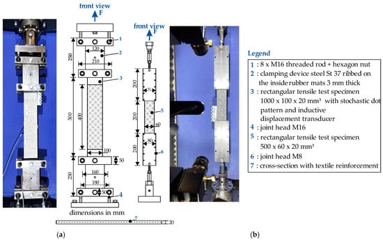
Figure 5.
Test setups for tensile strength tests on rectangular CTRC specimens. (a) RM adapted by [3]; (b) SRM.
For testing, the specimens were clamped in steel plates in the upper and lower load introduction areas over a length of 250 mm for RM and 150 mm for SRM. A torque of 100 Nm was applied for RM and 25 Nm for SRM, given their 20 mm thickness. Two LVDTs with a measuring length of 400 mm were installed at the backside of the RM specimens, parallel to the testing direction. Tensile strength tests were carried out using a 150 kN universal testing machine Zwick Z150 TL, maintaining a displacement control rate of 2 mm/min until the specimens’ failure occurred. The load and crosshead displacement were recorded in the software TestXpert® and then transferred to the DIC software. In the analysis, the x-axis was defined along the tensile direction, with the y-axis oriented perpendicular to it.
3.1.2. Tensile Test with Defined Crack Width
In order to validate the automated crack evaluation tool and threshold parameters used for crack width evaluation, tensile tests were conducted on two steel plates extending from each other for a defined crack. The steel plates, as shown in Figure 6, were separated at a crosshead displacement of 0.1 mm/min, ranging from 0 to 1.2 mm crosshead displacement. For the tests, a universal testing machine Zwick ZMART.Pro with a 10 kN load cell was used and two LVDTs were installed at the backsides of plates, parallel to the testing direction with a measuring length of 2 mm. The testing was performed concurrently with the optical measuring system Aramis® and a stochastic pattern was applied on the steel plates. The load and the crosshead displacement were recorded in the TestXpert® software V3.71 and then transferred to the DIC software.
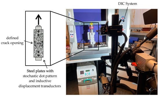
Figure 6.
Test setup for tensile testing of defined crack width.
3.1.3. Optical 3D Deformation Analysis
To analyze the full-field deformation of the surface during tests, the contact-free, optical 2D/3D-measuring system ARAMIS® from GOM GmbH was used. This system determined the exact load- and time-dependent measurements of crack formation and development.
The optical measurement system monitors surface deformation by analyzing captured images of facets (square image sections) identified using characteristic points (gray-level distribution), shown in Figure 7. When the 2D coordinates of the same facet are available, photogrammetric methods are employed to compute corresponding 3D coordinates. To facilitate this process, a random stochastic pattern was applied to the measurement area [3,31].
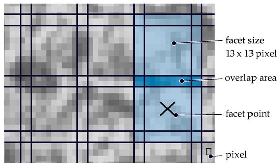
Figure 7.
Description of facets, pixel and overlap areas of optical 3D-measuring system.
Before starting the experiments, the measurement system was calibrated with calibration plates depending on the test setups, with RM and SRM completely enclosing the measuring area of the CTRC expansion specimens, as summarized in Table 4. During the tests, the deformation on the formwork side of the specimen was recorded with a frequency of 5 Hz.
Table 4.
Calibration parameters for the optical 3D-measurements.
3.2. Automated Crack Evaluation Tool for Optical 3D-Deformation Analysis
In the context of the parameter study for the evaluation of TRC crack distribution, a software tool was developed to perform the analysis process automatically. As mentioned above, this automated crack evaluation tool for DIC is referred to as ACE. ACE encompasses the processing of measurement data from the respective laboratory experiments using the DIC software as well as the analysis of crack widths and distribution. The following objectives have been established for this purpose:
- Importing measurement data as facet points from the DIC software;
- Processing the point coordinates of facet points in relation to the x and y axes within a coordinate system positioned on the test specimen;
- Storing the measured strains for each facet point and other data such as force, crosshead displacement, and LVDTs;
- Automatically identifying the positions of cracks and describing them using the point coordinates within the finalized crack image;
- Calculating the crack width during the test.
ACE was developed using the programming environment MATLAB® R2021b by MathsWorks, Inc. The user interface was created with the MATLAB® App Designer and linked with the programmed functions. The fundamental concept of the program was based on the principles of object-oriented programming (OOP). The objective of OOP is to represent real-world objects using data structures on a computer. This was achieved by creating classes that define the properties of an object. The MATLAB programming environment provides tools to implement OOP using classes, methods and functions [32,33].
For evaluation in ACE, in an initial step, measurement data such as force, crosshead movement, LVDTs, and major strain for each individual measurement step of the surface component created within the DIC software were exported in the form of tables. The coordinates of all facet points have subsequently been stored in one table for each measurement step.
3.2.1. Algorithms of ACE
ACE is based on several classes and functions; the concepts and operations of these are explained in the following and depicted in Figure 8.
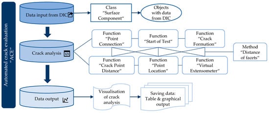
Figure 8.
Overview of ACE architecture.
In the first step, the exported tables are read using the “Surface Component” class. The data from the table are sorted in ascending order and assigned to the attributes of the object in this class. For each individual table, a separate object is created within this class. Additionally, within the “Surface Component” class, the average distance between the individual imported facet points is calculated. This distance is referred to as facet spacing in ACE.
The central element of ACE is the “Point Connection” function, whereby an algorithm is employed to determine the positions of cracks based on the facet point pattern of the measurement step at the end of the laboratory test. The facet points are arranged in a predetermined pattern within the DIC measurement system, as shown in Figure 9. For each individual facet point, the major strain is deposited in ACE. In Figure 9a, the facet points of the surface component are depicted with colors representing the magnitude of the major strain. Following the crack analysis described in Section 1, the crack distribution is determined using the scaling factor of the major strain. Provided that areas with cracks exhibit higher strain values, cracks within the measurement area can be identified using this approach. Therefore, a threshold scaling factor for the major strain is established. Exceeding this value, it is considered that cracks have occurred. The analysis of this threshold value is detailed in Section 4.1.
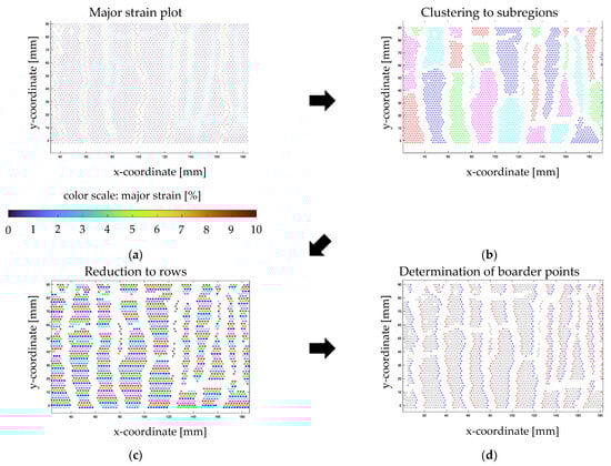
Figure 9.
Visualization of evaluation method ACE: (a) facet points with highlighted major strains from 1 to 10%. (b) Clustering to subregions. (c) Reduction to rows. (d) Determination of boarder points.
For further analysis, all facet points exceeding the threshold of major strain are initially removed, and the resulting crack image is divided into subregions. The subregions, as depicted in Figure 9b, are then subjected to further examination. The subregions are separated by the cracks and subdivided into connected facet point clouds. The maximum distance between facet points within a subregion is 1.5 times the facet spacing. To achieve this, for each individual facet point, the facet points that do not exceed this maximum distance are determined. Subsequently, a network is formed, representing a connected area. Isolated facet points that cannot form a subregion are not considered in the further stages of ACE. The subregions are numbered from left to right in ascending order. In a subsequent step, the subregions are divided into rows, see Figure 8c. To achieve this, all facet points belonging to a common subregion whose y-coordinate differs by less than 0.3 times the facet spacing and whose x-coordinate differs by less than 1.5 times the facet spacing are assigned to a common row. As shown in Figure 9d, the points with the smallest x-coordinate mark the beginning of a row, while the points with the largest x-coordinates signify the end of a row.
The edge points of a row, identified in this manner, are assigned to a crack boarder in the next step. The starting point of each crack boarder is defined by the first and last points of the highest y-coordinate within each subregion. Starting from such a point, additional points of the crack boarder are successively added along a chain. The subsequent algorithm criteria are considered when assigning the next point to the crack boarder:
- Facet points belong to the same subregion;
- The next facet point can be assigned to the same group in terms of the beginning or end of a row. Typically, facet points on the right crack boarder are at the beginning of a row, while facet points on the left crack boarder are at the end of a row. Points located in a row with only one point may belong to the right and left crack boarders of two different cracks;
- Since the chain is traversed from higher to smaller y-coordinates, the subsequent point has a smaller y-coordinate than the starting point or the previous point;
- Regarding the y-coordinate, the facet point must be a maximum of 2 times and a minimum of 0.5 times the facet spacing away from the starting point or the previous point;
- In terms of the x-coordinate, the facet point must be a maximum of 4 facet points away from the starting point or the previous point.
If these conditions apply to multiple points, the point with the smallest distance takes precedence. Additional points are added to the crack boarder until none of the conditions can be met by the facet point. Furthermore, it should be noted that the beginning of each row in the first subregion and the end of each row in the last subregion are not considered, because these points describe the boundary region of the measurement area. In cases where cracks do not extend continuously across the entire width of the measurement area, the described steps are repeated from the bottom edge of the subregions. These assigned points are referred to as boarder points (BP).
In the subsequent stages of this function, each point on the left crack boarder is paired with a corresponding point on the right crack boarder, depicted in Figure 10. In Figure 10a, the BP are highlighted in red and blue connected by a pink line. These two points together are referred to as a BP couple. The facet points of each surface component are distinguished with a unique point ID. For the identified BPs and pairs, a separate table is created for each crack. Each row in these tables contains the point IDs of both BPs within a BP couple. These tables are stored as distinct attributes within the valuated object of the class.
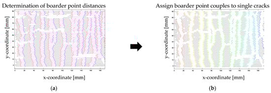
Figure 10.
Visualization of the crack assignment: (a) BP couple; (b) BP couples assigned to cracks.
An additional function in ACE determines the positions of individual points over the laboratory test. For each facet point, a corresponding point in the previous measurement images is sought. The resulting chain of points is stored in a matrix.
The “Crack Formation” function forms the basis for tracking the BPs over the duration of the test to determine changes in crack width. Starting from objects in the “Surface Component” class, the crack positions are tracked in subsequent measurement images. To achieve this, as shown in Figure 11a, the mean value between two BPs of a BP couple is determined. Based on this, the two nearest points are searched for in the point coordinates of the surface component of object 2. The following three conditions are applied to determine the BP couple:
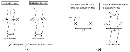
Figure 11.
Determination of crack width with ACE: (a) Crack width calculation; (b) locations of BP couples for the evaluation stages.
- The sought BPs do not exceed the limit value of major strain;
- The y-coordinate of the sought BPs deviates by a maximum of 0.5 times the facet spacing from the y-coordinate of the mean value;
- A point with a greater x-coordinate and a point with a smaller x-coordinate than the mean value is sought.
Based on this, the distance between two BPs of a BP couple a0 is calculated. The algorithm computes the individual distance of all BP couples for all cracks across the entire evaluation stages. The distance is determined using Equation (5) with the distance of BPs (atotal), distance of BPs in the first evaluation stage (a0), distance of BPs (a), and the respective evaluation stage (i) exemplified in Figure 11b.
atotal(i) = a(i) − a0
Furthermore, ACE facilitates the placement of a virtual extensometer within the measurement area by computing the distance between two selected facet points throughout the evaluation stages (i). Therefore, the distance of selected facet points ΔL is divided by the distance of the first evaluation stage (l1).
ε(i) = ΔL/l1
The results of calculations obtained with ACE can be saved for further evaluations and displayed graphically. The following graphics can be generated in ACE:
- Facet points (with and without color representation of the major strain);
- Placement of virtual extensometer;
- Facet points with highlighted BPs, crack boarders, and BP couple;
- Stress and crosshead displacement across the evaluation stages;
- Crack distribution and average crack width;
- Average strain of virtual displacement sensors;
- Combinations of the mentioned individual data.
3.2.2. Validation of ACE
To validate ACE, the manual analysis of crack width was compared to the results of ACE for tensile strength tests on CTRC. The manual evaluation method, described in the introduction, represents the current state of art and is herein applied in the field of textile reinforced concrete tensile testing. Hence, this method was used to compare the developed tool with the results of manual evaluation. This comparison was based on the evaluated crack widths arising in relation to the strain, as shown in Figure 12. The crack widths evaluated with ACE were in accordance with the results obtained manually. Hence, ACE was employed for the parameter study in this paper.
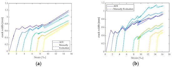
Figure 12.
Comparison of the results of manual evaluation in the DIC software and ACE: (a) CTRC-1; (b) CTRC-2.
4. Results
4.1. Scaling Factor for Major Strain in Crack Analysis
To determine the scaling factor for major strain, a parameter study was conducted using tensile strength tests with defined crack widths and CTRC tensile strength tests. Through measurements with the DIC software, only the surface crack formation was recorded. However, based on Morales Cruz’ and Jesse’s [3,34] findings via rectangular CTRC tensile strength tests, it is reasonable to assume that the crack behavior remains consistent with depth. Tensile strength tests revealed a consistent crack pattern with depth from the lateral views due to the rectangular specimen shape.
In this analysis, it was observed that cracks in the CTRC surface originated from strain bands. As shown in Figure 13, the formed strain bands are highlighted and the major strain increased as the tensile force increased, leading to the development of additional strain bands.
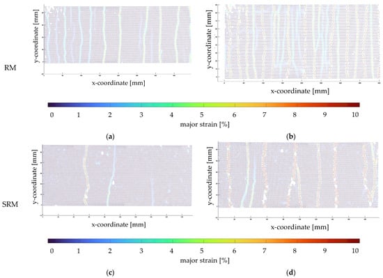
Figure 13.
Strain bands on CTRC specimens: (a) crack distribution at 1650 N/mm2; (b) crack distribution at 4125 N/mm2; (c) crack distribution at 1200 N/mm2; (d) crack distribution at 4000 N/mm2.
It can be observed that a crack formed at each strain band. A crack suddenly appeared on the surface and the major strain in the crack region began to rise. It was determined that the initiation of the crack occurred when the fracture strain of the existing repair mortar was exceeded [35]. Furthermore, in subsequent phases of the experiment, the major strain in this crack continued to increase, and the region with altered strain expanded. This phase marked the point at which the crack width started to increase. A higher number of strain bands led to smaller crack widths and a more favorable crack distribution.
To determine the scaling factor of major strain for the crack width calculation, the variation in major strain within a specific section of a specimen at the same evaluation stage is depicted in Figure 14. The facet points highlighted in red indicate those excluded from the crack width calculations based on the scaling factor. The adjacent facet points form the crack boarders.
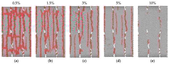
Figure 14.
Facet points over scaling factors highlighted in red: (a–e) Varying major strains.
It can be observed that more facet points were developed with smaller factors. To analyze the effects of the scaling factor on crack width, laboratory experiments were conducted with defined crack widths as described in Section 3.1.2, and the crack width was determined using ACE with varying scaling factors for major strain values, as depicted in Figure 15. The objective was to establish the correlation between crack width in the results of the laboratory experiment and in the results of the evaluation in ACE with linear crack width opening.
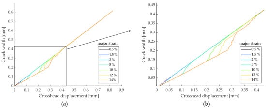
Figure 15.
Comparison of defined crack width with ACE calculated with 15 × 15-pixel facet size and 3-pixel facet overlap: (a) overview; (b) detail.
The results indicate that increasing the major strain values led to smaller crack widths as calculated by ACE with identical crosshead displacement. Once the crack width reached 0.4 mm, the crack width measurements aligned. This could be attributed to the fact that a smaller scaling factor led to more facet points exceeding the limit and being defined as cracks, as shown in Figure 14. Smaller major strain values were reached at an earlier stage, resulting in smaller crack width. Beyond a crack width of 0.4 mm, the influence of varying limits decreased, as higher limits were also exceeded due to the increasing strain.
These results align with those of individual crack width analyses conducted in CTRC laboratory experiments with 19 × 19-pixel facet sizes and 3-pixel facet overlap in ACE, as shown in Figure 16 and Figure 17.
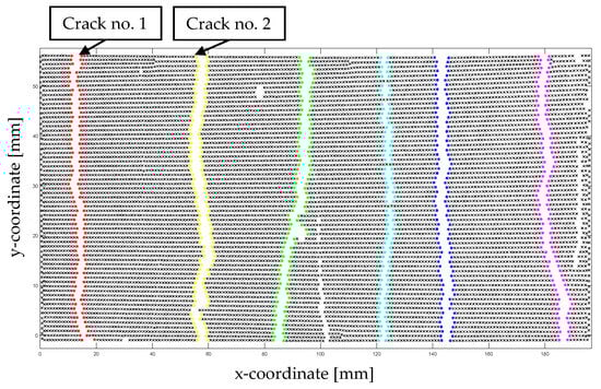
Figure 16.
Crack distribution of expansion specimen.
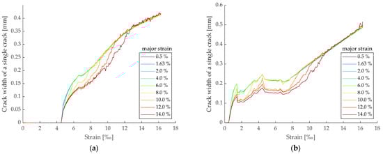
Figure 17.
The average crack widths of selected cracks in the CTRC tensile strength tests analyzed with varying major strain values: (a) Crack analysis of crack no. 1; (b) crack analysis of crack no. 2.
The results derived using a limit value of 0.5% allow for consistent crack width calculations and enable the detection of fine cracks. However, choosing a scaling factor smaller than 0.5% is not recommended, as it may introduce inaccuracies via measurement noise. The facet points exhibit local strains due to the minimal measurement inaccuracies within the DIC system. Based on the research findings, major strain values smaller than 0.5% cannot be considered as indicative of crack development. Setting the threshold below 0.5% enables us to identify nearly all points as cracks, as the measurement noise cannot be eliminated.
4.2. Facet Size
To determine the facet size for crack width analysis, facet sizes from 11 × 11 pixels to 23 × 23 pixels were investigated. Thereby, the facet size can be inferred to significantly affect the number of facet points on the measurement area. As shown in Table 5, a smaller facet size of 11 × 11 pixels resulted in a six-fold higher number of facet points compared to 23 × 23 pixels.
Table 5.
Number of facet points in the measurement area at the start of the laboratory experiment.
An increasing number of facet points resulted in a larger dataset to be analyzed. Therefore, it is important to find a balance between having as many data points as possible while keeping the data manageable. To identify this balance, comparative crack distributions on a CTRC specimen with a 0.5% scaling factor are depicted in Figure 18. The individual cracks are highlighted with different colors.
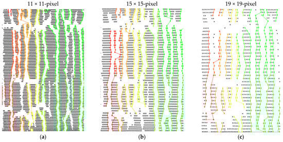
Figure 18.
Crack formation with varying facet sizes evaluated with ACE: (a) 11 × 11-pixel; (b) 15 × 15-pixel; (c) 19 × 19-pixel.
It can be seen that the choice of facet size has an impact on the revealed crack distribution. Particularly, cracks that were close to each other may have not been identified and analyzed as a result of the facet size. This could lead to an underestimation of the crack number when using larger facet sizes compared to evaluations with smaller facet sizes. In the example depicted in Figure 18, out of 27 cracks that were detected within the measurement area using a facet size of 13 × 13 pixels, only 22 cracks were visible when using a facet size of 19 × 19 pixels. A crack may go undetected either because two closely spaced cracks cannot be distinguished from each other, or because the areas between the cracks with excessive major strain values may not be captured with greater facet spacings. Alternatively, the facet spacing may be selected to be sufficiently large that, visually, the crack appears to run between the facet points, and the crack boarders do not clearly stand out from the point distribution.
Furthermore, the average crack widths of an individual crack were determined with varying facet sizes, as depicted in Figure 19. The analyzed crack widths were aligned, as seen for cracks no. 1 and 2. The scaling factor of the major strain was adjusted proportionally for each chosen facet size to equalize the influence, with a facet overlap of three pixels.
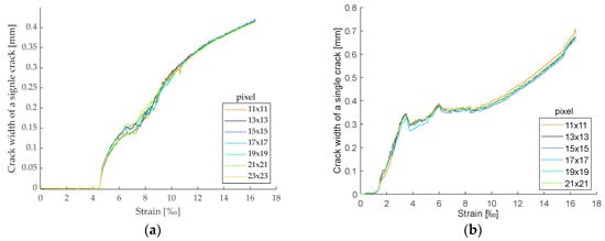
Figure 19.
Average crack width of selected cracks from CTRC tensile strength test with different facet sizes: (a) crack analysis of crack no. 1; (b) crack analysis of crack no. 2.
Therefore, the selection of the facet size for this evaluation was guided by optical criteria and the practical computational capacity accessible to the user. As a result, a facet size of 15 × 15 pixel or smaller is recommended.
4.3. Facet Overlap
The analysis of the facet overlap from 1 to 7 pixels was examined through crack width analyses for cracks no. 1 and 2, using a 15 × 15-pixel facet size and a 0.5% scaling factor of major strain. With a 1-pixel facet overlap, the crack width varied from 0.35 mm by approximately 0.02 mm. These variations are attributed to the assignment of facet points in ACE, and are not further considered in the analysis. The results show that a three- to seven-pixel overlap led to identical crack widths with increasing strain, as depicted in Figure 20. In addition, the number of data points in the evaluation increased with an increasing pixel overlap. Based on the identical crack widths and the increasing data number, a facet overlap of three pixels is recommended.
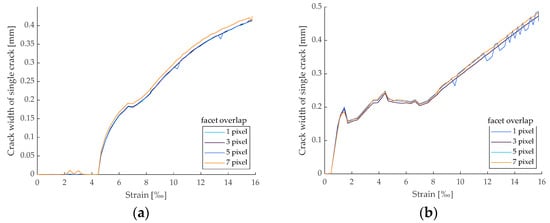
Figure 20.
Average crack widths of cracks selected from the CTRC tensile strength tests with different facet overlaps: (a) crack analysis of crack no. 1; (b) crack analysis of crack no. 2.
5. Conclusions and Outlook
In this study, the investigation focused on probing the impacts of key parameters, such as threshold value for crack detection, facet size and facet overlap, in textile reinforced concrete crack analysis via measurements using DIC software. For this purpose, an automated crack evaluation software was developed and validated. The findings provide valuable insights into the cracking behaviors of tested materials, and offer innovative guidance for the selection of appropriate parameters in crack width analysis.
The key findings of this study can be summarized as follows:
- ACE, as a novel tool, has been developed based on object-oriented programming. ACE enables the import of measurement data from the DIC software, facilitates facet point processing, and automates crack positions’ identification and crack width calculation for evaluation. In this process, the average crack width is calculated in terms of the entire cross-section. ACE was successfully validated for crack width analysis with manual evaluations using the DIC software;
- Strain bands formed during the laboratory experiments, which subsequently gave rise to individual cracks. The abrupt initiation of cracks led to the formation of strain bands, followed by a continuous increase in the major strain of facet points. The evaluation of these strain bands revealed that the presence of multiple small cracks results in a lower maximum major strain of the facet points in strain bands;
- Variations in the major strain scaling factor have a significant impact on crack width. An increase in this value leads to a smaller average crack width at the same strain stage. However, beyond a crack width threshold of 0.4 mm, the influence of the scaling factor becomes less pronounced. To achieve optimal crack width analysis, a scaling factor of 0.5% is recommended;
- The choice of facet size in the analysis of crack widths was proven to be a decisive factor in the evaluation of measurement data. Thereby, the facet size influences the number of data points available for analysis. The selected facet size should achieve a compromise between the detection of even minor cracks and the maintenance of manageable computational demands. In this context, based on the optical criteria, a facet size of 15 × 15 pixels or smaller is recommended;
- This parameter study on facet overlap in relation to crack width evaluation has demonstrated that for overlaps of three pixel or more, there was no detectable influence. Consequently, it is advisable to adopt a three-pixel overlap parameter to ensure optimal results. This selection ensures efficiency and precision in crack width evaluation within DIC measurements.
Future investigations should assess the applicability of ACE in additional areas of DIC measurements for construction materials. Moreover, the integration of advanced features, such as automating assessments across entire experimental series, presents a promising avenue for further enhancements. In these additional areas, the investigated parameters should be verified and, if necessary, adapted to the different material combinations and laboratory experiments.
Author Contributions
Conceptualization, methodology, software, validation, formal analysis, investigation, resources, data curation, writing—original draft preparation, visualization, A.D.; writing—review and editing, supervision, project administration, A.D. and M.R. All authors have read and agreed to the published version of the manuscript.
Funding
This research received no external funding.
Data Availability Statement
The data presented in this study are available in the article.
Conflicts of Interest
The authors declare no conflict of interest.
References
- Nyathi, M.A.; Bai, J.; Wilson, I.D. Concrete Crack Width Measurement Using a Laser Beam and Image Processing Algorithms. Appl. Sci. 2023, 13, 4981. [Google Scholar] [CrossRef]
- Yang, X.; Li, H.; Yu, Y.; Luo, X.; Huang, T.; Yang, X. Automatic pixel-level crack detection and measurement using fully convolutional network. Comput.-Aided Civ. Infrastruct. Eng. 2018, 33, 1090–1109. [Google Scholar] [CrossRef]
- Morales Cruz, C. Crack-Distributing Carbon Textile Reinforced Concrete Protection Layers. Ph.D. Thesis, RWTH Aachen University, Aachen, Germany, 2020. [Google Scholar]
- Morales Cruz, C.; Raupach, M. Influence of the surface modification by sanding of carbon textile reinforcements on the bond and load-bearing behavior of textile reinforced concrete. In Proceedings of the MATEC Web of Conferences: Concrete Solutions 2019—7th International Conference on Concrete Repair, Cluj, Romania, 30 September–2 October 2019; p. 10. [Google Scholar]
- Ortlepp, R.; Hampel, U.; Curbach, M. A new approach for evaluating bond capacity of TRC strengthening. Cem. Concr. Compos. 2006, 28, 589–597. [Google Scholar] [CrossRef]
- Hampel, U.; Maas, H.-G. Cascaded image analysis for dynamic crack detection in material testing. ISPRS J. Photogramm. Remote Sens. 2009, 64, 345–350. [Google Scholar] [CrossRef]
- Munawar, H.S.; Hammad, A.W.; Haddad, A.; Soares, C.A.P.; Waller, S.T. Image-based crack detection methods: A review. Infrastructures 2021, 6, 115. [Google Scholar] [CrossRef]
- Golding, V.P.; Gharineiat, Z.; Munawar, H.S.; Ullah, F. Crack detection in concrete structures using Deep Learning. Sustainability 2022, 14, 8117. [Google Scholar] [CrossRef]
- Scislo, L. Quality assurance and control of steel blade production using full non-contact frequency response analysis and 3D laser doppler scanning vibrometry system. In Proceedings of the 11th IEEE International Conference on Intelligent Data Acquisition and Advanced Computing Systems: Technology and Applications (IDAACS), Cracow, Poland, 22–25 September 2021; pp. 419–423. [Google Scholar]
- Longo, R.; Vanlanduit, S.; Vanherzeele, J.; Guillaume, P. A method for crack sizing using Laser Doppler Vibrometer measurements of Surface Acoustic Waves. Ultrasonics 2010, 50, 76–80. [Google Scholar] [CrossRef] [PubMed]
- Maas, H.G. On the potential of photogrammetric techniques in civil engineering material testing. Bautechnik 2012, 89, 786–793. [Google Scholar] [CrossRef]
- Sohn, H.G.; Lim, Y.M.; Yun, K.H.; Kim, G.H. Monitoring crack changes in concrete structures. Comput.-Aided Civ. Infrastruct. Eng. 2005, 20, 52–61. [Google Scholar] [CrossRef]
- Kim, H.; Ahn, E.; Cho, S.; Shin, M.; Sim, S.-H. Comparative analysis of image binarization methods for crack identification in concrete structures. Cem. Concr. Res. 2017, 99, 53–61. [Google Scholar] [CrossRef]
- Wang, P.; Huang, H. Comparison analysis on present image-based crack detection methods in concrete structures. In Proceedings of the 3rd International Congress on Image and Signal Processing, Yantai, China, 16–18 October 2010; pp. 2530–2533. [Google Scholar]
- Barazzetti, L.; Scaioni, M. Crack measurement: Development, testing and applications of an automatic image-based algorithm. ISPRS J. Photogramm. Remote Sens. 2009, 64, 285–296. [Google Scholar] [CrossRef]
- Godek, E.; Felekoglu, K.T. Effect of camera resolution on the determination of mechanical and multiple crack properties of Engineered Cementitious Composites via Digital Image Correlation. Hittite J. Sci. Eng. 2023, 10, 117–124. [Google Scholar] [CrossRef]
- Morales Cruz, C.; Kriescher, K.; Raupach, M. Instandsetzung des östlichen Umlaufkanals der Westkammer der Schleuse Anderten in Anlehnung an das BAW-Merkblatt MITEX. In Proceedings of the 8. Kolloquium Erhaltung von Bauwerken, Esslingen, Germany, 14–15 February 2023. [Google Scholar]
- Ohno, M.; Li, V.C. A feasibility study of strain hardening fiber reinforced fly ash-based geopolymer composites. Constr. Build. Mater. 2014, 57, 163–168. [Google Scholar] [CrossRef]
- Zhu, D.; Liu, S.; Yao, Y.; Li, G.; Du, Y.; Shi, C. Effects of short fiber and pre-tension on the tensile behavior of basalt textile reinforced concrete. Cem. Concr. Compos. 2019, 96, 33–45. [Google Scholar] [CrossRef]
- Wilhelm, T. Ein Experimentell Begründetes Mikromechanisches Modell zur Beschreibung von Bruchvorgängen in Beton bei Äußerer Krafteinwirkung. Ph.D. Thesis, Technische Universität Darmstadt, Darmstadt, Germany, 2006. [Google Scholar]
- Domski, J.; Katzer, J. Validation of aramis digital image correlation system for tests of fibre concrete based on waste aggregate. Key Eng. Mater. 2018, 761, 103–110. [Google Scholar] [CrossRef]
- Jesse, F.; Kutzner, T. Digital photogrammetry in construction engineering—Influence of major system parameters and accuracy potential in applications. Bautechnik 2013, 90, 703–714. [Google Scholar] [CrossRef]
- Hampel, U. Application of Photogrammetry for Measuring Deformations and Cracks during Load Tests in Civil Engineering Material Testing. Ph.D. Thesis, Technische Universität Dresden, Dresden, Germany, 2008. [Google Scholar]
- TR IH: Technische Regel—Instandhaltung von Betonbauwerken (TR Instandhaltung)—Teil 1: Anwendungsbereich und Planung der Instandhaltung; Deutsches Institut für Bautechnik (DIBt): Berlin, Germany, 2020.
- TR IH: Technische Regel—Instandhaltung von Betonbauwerken (TR Instandhaltung)—Teil 2: Merkmale von Produkten oder Systemen für die Instand-Setzung und Regelungen für deren Verwendung; Deutsches Institut für Bautechnik (DIBt): Berlin, Germany, 2020.
- Technical Product Data Sheet—Solidian. Available online: https://solidian.com/downloads/ (accessed on 12 October 2023).
- DIN EN 1015-3; Methods of Test for Mortar for Masonry—Part 3: Determination of Consistence of Fresh Mortar (By Flow Table). DIN Deutsches Institut für Normung e.V: Berlin, Germany, 2007; German Version.
- DIN EN 1015-6; Methods of Test for Mortar for Masonry—Part 6: Determination of Bulk Density of Fresh Mortar. DIN Deutsches Institut für Normung e.V: Berlin, Germany, 2007; German Version.
- DIN EN 1015-7; Methods of Test for Mortar for Masonry—Part 7: Determination of Air Content of Fresh Mortar. DIN Deutsches Institut für Normung e.V: Berlin, Germany, 1998; German Version.
- DIN EN 1015-11; Prüfverfahren für Mörtel für Mauerwerk—Teil 11: Bestimmung der Biegezug- und Druckfestigkeit von Festmörtel. DIN Deutsches Institut für Normung e.V: Berlin, Germany, 2020.
- GOM mbH. GOM Correlate Professional. V8 SR1 Manual Basic; GOM mbH: Braunschweig, Germany, 2015. [Google Scholar]
- Register, A.H. A Guide to MATLAB Object-Oriented Programming; Chapman & Hall/CRC: Boca Raton, FL, USA, 2007. [Google Scholar]
- Stein, U. Objektorientierte Programmierung Mit MATLAB: Klassen, Vererbung, Polymorphie; Carl Hanser Verlag GmbH Co. KG: Munich, Germany, 2015. [Google Scholar]
- Jesse, F. Bearing Behavior of Filament Yarns in a Cementitious Matrix. Ph.D. Thesis, Technische Universität Dresden, Dresden, Germany, 2005. [Google Scholar]
- Lange, J. Techniques for Measurement and Analysis in Crack and Fibre Detection at Concrete Elements. Ph.D. Thesis, RWTH Aachen University, Aachen, Germany, 2010. [Google Scholar]
Disclaimer/Publisher’s Note: The statements, opinions and data contained in all publications are solely those of the individual author(s) and contributor(s) and not of MDPI and/or the editor(s). MDPI and/or the editor(s) disclaim responsibility for any injury to people or property resulting from any ideas, methods, instructions or products referred to in the content. |
© 2023 by the authors. Licensee MDPI, Basel, Switzerland. This article is an open access article distributed under the terms and conditions of the Creative Commons Attribution (CC BY) license (https://creativecommons.org/licenses/by/4.0/).