Temperature Response of Double-Layer Steel Truss Bridge Girders

Abstract

Double-layer steel truss continuous girders are prone to significant temperature stress, deviation, torsion, and warping, thus causing adverse temperature structural responses, and also affecting the safety and durability of bridge structures. This paper presents an investigation on time-dependent characteristics in the temperature field and temperature response of double-layer steel truss continuous bridge girders, fully considering the shielding effect subjected to different solar radiation angles during the high-temperature season. The time-dependent thermal boundary conditions and support conditions provided for the steel truss bridge structure were determined. Subsequently, a thermal analysis model for the entire structure of double-layer steel truss continuous girders was established to attain the temperature distribution law. The research results show that significant differences occur in the position and temperature difference of temperature gradients exhibited in the vertical, horizontal, and longitudinal directions in the double-layer steel truss bridge structure. The temperature distribution pattern within the chord section is mainly influenced by the environmental temperature and solar radiation intensity, along with the heat exchange between different panels. Thereafter, a validated temperature gradient formula for the component section has been proposed. The time-dependent laws in structural displacement, stress, and rotation angle under daily temperature cycling conditions have been revealed, thereby providing a theoretical basis for the life cycle construction and safety maintenance of double-layer steel truss structure bridges.

1. Introduction

The steel truss girder possesses the advantages of being lightweight, having a long span, and exhibiting high stiffness [1], which makes it widely used in double-deck bridges [2]. Due to factors such as solar radiation, atmospheric temperature [3], wind speed, and other environmental conditions, significant variations occur in its temperature field [4,5], resulting in noticeable temperature discrepancies among components. Moreover, this nonlinear temperature distribution significantly impacts the internal forces and alignment of the bridge structure, leading to a reduction in loading capacity and even structural failure [6]. Therefore, the timely evaluation and control of the influence of temperature loads on the safety and durability of bridge structures at each stage throughout their life cycle are crucial for ensuring safe construction and maintenance.

Currently, the existing research both domestically and internationally primarily focuses on the temperature field and temperature effects of concrete bridges and steel–concrete composite bridges [7,8,9,10,11,12]. However, there is insufficient investigation into the temperature field of double-layer steel trusses. Through extensive theoretical analysis, numerical simulation, and monitoring techniques, the typical temperature distribution of the box girder and steel–concrete composite girder is presented. It is acknowledged that solar radiation, external environmental conditions, and bridge type directly influence bridge temperatures [13]. To more accurately and efficiently depict the actual temperature field during the construction and operation stages of bridge structures, we employ shadow recognition algorithms and bounding box algorithms, as well as hidden algorithms in temperature field simulations [14]. Various studies have proposed calculation methods considering transverse and vertical temperature loads, along with thermal stresses. Research indicates that, due to shielding effects, the temperature fields differ significantly between double-layer steel truss continuous girders compared to those of steel–concrete composite girders or concrete box girders [15,16].

Bridge design codes from various nations offer models of temperature distribution curves for the bridge’s thermal field, particularly focusing on common sections like box girders and steel–concrete composite girders [17,18,19,20]. Regional factors, pavement types, concrete thicknesses, and approaches employed in calculating negative gradient loads contribute to significant variations. Nevertheless, current codes do not include explicit guidelines concerning the temperature gradient of steel trusses. Conventional studies assume effective heat transfer properties in steel trusses while assuming a uniform temperature difference among their members. By conducting numerical calculations and monitoring real bridges, Zhu et al. discovered significant discrepancies between the calculated deformation of the main girder and the overall temperature fluctuation model when subjected to non-uniform temperature fields caused by solar radiation on railway steel truss suspension bridges [21]. Based on data obtained from a health-monitoring system installed on the main channel bridge of the Husutong Yangtze River Railway Bridge, Zhang et al. investigated the temporal and spatial distribution of the temperature field in a double-layer steel truss structure [22]. The results demonstrate that the temperature distribution in the steel truss girder exhibits temporal lag and spatial variations in both the horizontal and vertical directions. Through the extensive monitoring of railway steel truss bridges, Wang et al. [23,24,25] observed significant positive and negative temperature discrepancies among truss members, attributing the lateral temperature gradient between trusses as the primary factor influencing their lateral rotation angle. Consequently, it is imperative to investigate the time-varying characteristics of temperature fields and their effects on double-layer steel truss continuous girders under shielding conditions.

The focus of this paper is to investigate the temperature field and response of a double-layer steel truss continuous girder under shielding effects using an advanced numerical simulation model. Firstly, a validated thermal analysis model is developed based on structural shielding analysis. Furthermore, the distribution of the temperature field in both the entire structure and important components is examined. Finally, the displacement distribution, temperature response characteristics of structural stress, and rotation angle at the end of the double deck caused by solar radiation are explored. The research findings provide a theoretical basis for the life cycle construction and safety maintenance of double-layer steel truss structures.

2. Thermal Analysis Model

The natural environment exhibits temporal variations in temperature, solar radiation, air humidity, and cloud thickness. These variations, combined with the shielding effect among bridge structures, lead to disparities in the received solar radiation intensity for each component. Consequently, the temperature field of bridges demonstrates intricate spatio-temporal characteristics. The numerical simulation method is employed to simulate the heat exchange process between the bridge and its surrounding environment, in order to obtain the time-varying temperature field of the double-layer steel truss continuous girder.

2.1. Environmental Temperature Model

Based on meteorological data [26] and on-site measurements in a specific region, the highest and lowest temperatures recorded during periods of extremely high-temperature weather [27] in the hot season are documented. The average maximum temperature is determined to be 41 °C, while the average minimum temperature is calculated as 27 °C. The ambient temperature at any given time is represented as:

$$T=\frac{1}{2}\left(T_{max}+T_{min}\right)+6.5\sin \left(\frac{\pi }{12}\left(t-9\right)\right)$$

(1)

where t (h) represents any time point within a day, and T_max and T_min (°C), respectively, denote the average maximum and minimum temperatures of extreme high-temperature weather during the high-temperature season.

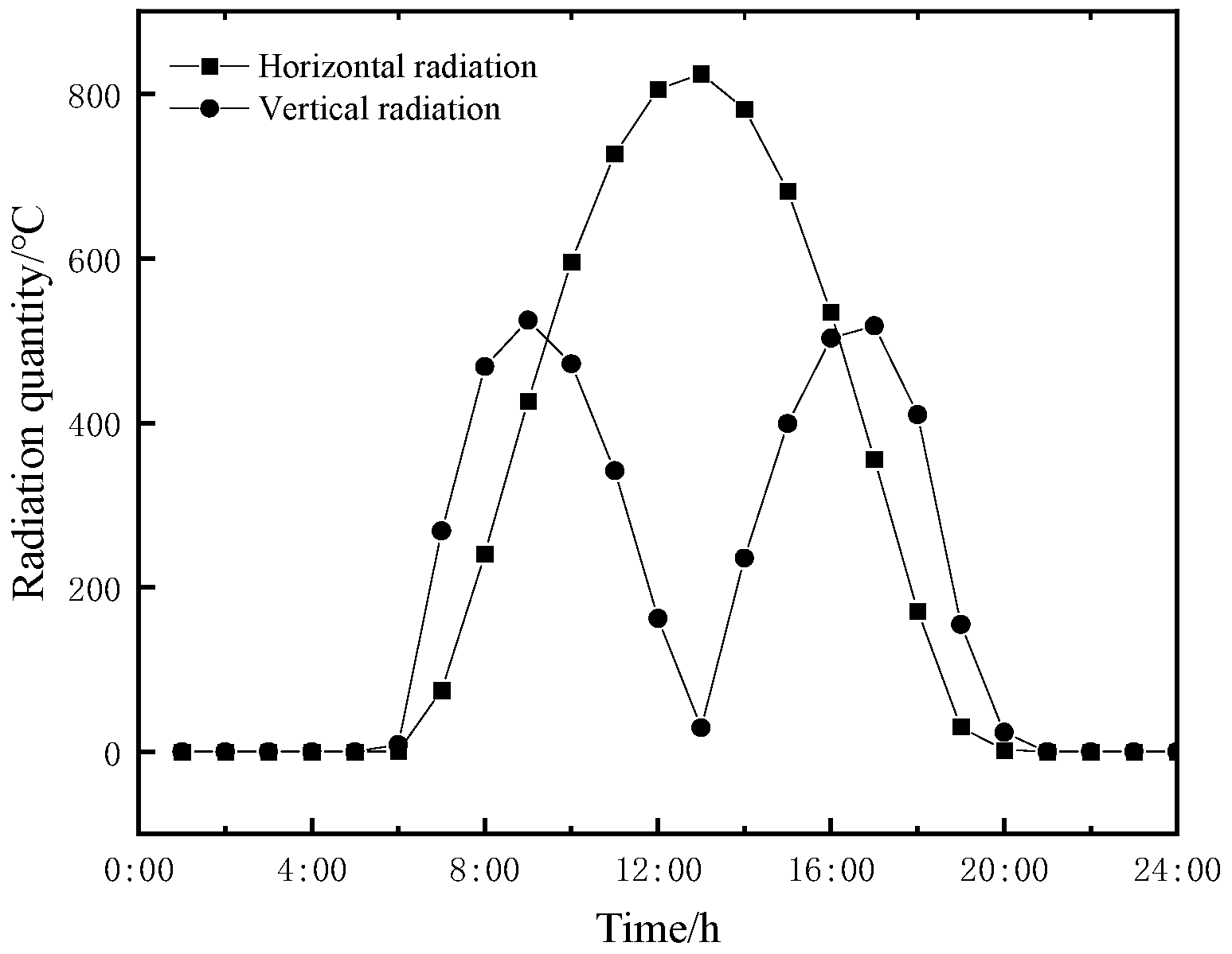
2.2. Solar Radiation

The solar radiation received by bridges is primarily categorized into direct solar radiation, diffuse solar radiation, and ground reflection. Considering the research focus on a double-deck steel truss continuous girder, it becomes imperative to account for the impact of inter-component shielding on solar radiant energy.

2.2.1. Direct Solar Radiation

Direct solar radiation refers to the energy an object receives directly through the atmosphere from the sun. It is expressed as follows:

$$I_m=I_0{0.9}^{t_u{k}_{a}m}\cos \alpha$$

(2)

where I₀ (W/m²) is the solar constant, I₀ = 1367 [1 + 0.33 cos(360 N⁄365)], N is the daily serial number, k_a (Pa) is the atmospheric relative pressure, m (m) is the optical path length, m = 1⁄sinβ, and α (°) is the solar radiation angle.

2.2.2. Diffuse Solar Radiation

Diffuse solar radiation comprises atmospheric scattering and ground reflection. The intensity of atmospheric scattering radiation is correlated with the angle θ formed between the receiving surface for radiation and the horizontal plane [28].

When θ = 0, the expression for atmospheric scattered radiation (W/m²) is:

$$I_{d0}=0.5I_0\sin \beta \frac{1-P_m}{1-1.4\log P}$$

(3)

where P_m and P, respectively, represent the atmospheric transparency coefficient and the composite atmospheric transparency coefficient, and their expressions are $P_m={0.9}^{t_u{k}_{a}m}$, $P={0.9}^{t_u{k}_a}$, and $\beta$ (°) is solar altitude angle.

When θ ≠ 0, the atmospheric scattering expression is:

$$I_{d\theta }=0.5I_{d\theta }\left(1+\cos \theta \right)$$

(4)

where $\theta$ (°) is the angle between the surface receiving scattered radiation and the horizontal plane.

The ground reflectivity will also affect the radiant intensity of solar scattering. The expression for the ground reflection intensity of any surface is:

$$I_r=0.5r_e\left(I_m+I_{d0}\right)\left(1-\cos \beta \right)$$

(5)

where $r_e$ is the reflectivity of surface objects.

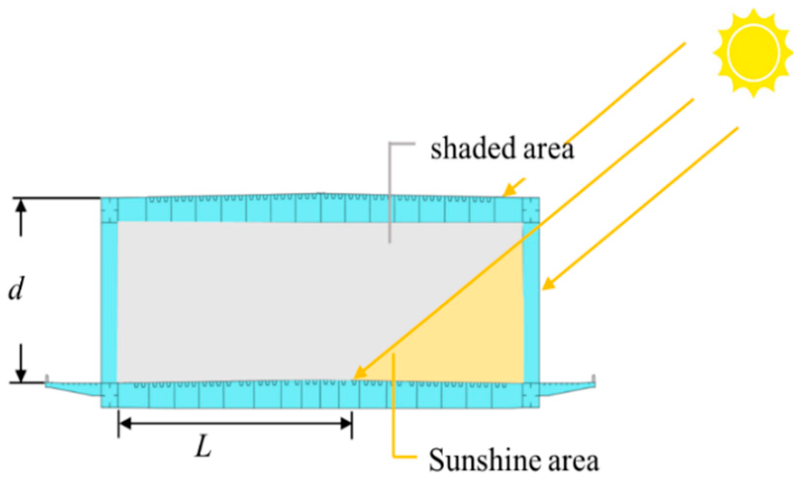
2.2.3. Double-Deck Shading Model

In the sunshine model, due to the continuous variation in the sun’s height, the lower deck becomes covered by the upper deck, resulting in a lateral temperature difference. Hence, it is imperative to establish a shading model for the upper deck, as depicted in Figure 1.

The shielding length L of the lower deck varies over time, expressed as:

$$L=d\frac{\tan \beta }{\cos \left({\gamma }_s-\gamma \right)\sin \delta +\cos \delta \tan \beta }$$

(6)

where d (m) is the height between the double-deck bridges, γ and γ_s (°) is the plane azimuth and solar azimuth angle, respectively, and δ (°) is the inclination angle of the plane.

2.2.4. Total Solar Radiant

The total radiant (W/m²) of the sunshine area is different from that of the shaded area, so the total expression is:

$$I=\left\{ \begin{array}{c}{I}_m+I_{d0}/I_{d\theta }+I_r Sunshine area \\ I_{d0}/I_{d\theta }+I_r Shaded areas\end{array}\right.$$

(7)

The radiation parameters in this article are based on data obtained during the summer solstice of 2022, specifically on the 188th day of the year and with a solar inclination angle of 23.44°. The bridge is situated at a latitude of 33°42′ N and a longitude of 107°36′ E, spanning from south to north directionally. The solar radiation incident upon different components of the bridge varies due to their respective angles ranging between 0° and 90°, resulting in diverse levels of radiant intensity. Figure 2 illustrates the temporal variation curve depicting both horizontal and vertical radiant intensities.

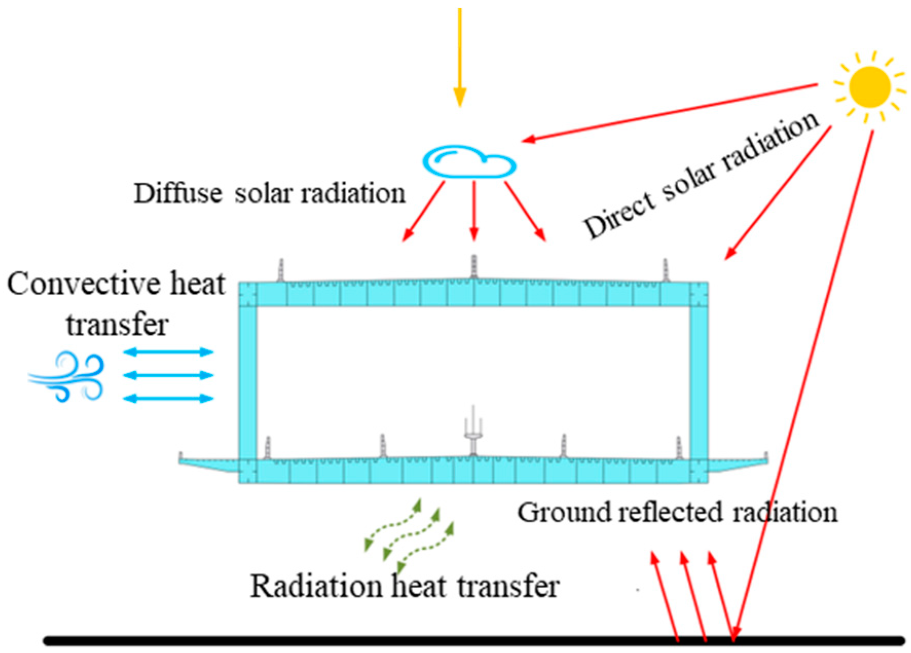
2.3. Simulation of External Thermal Boundary of Double-Layer Steel Truss

The heat exchange mode of the outer boundary of the model is divided into three types: solar radiation, convective heat transfer, and radiation heat exchange. The heat exchange model is shown in Figure 3.

2.3.1. Virtual Thermal Boundary

A virtual boundary is constructed outside the component. The virtual boundary temperature is caused by solar radiation, which is called the comprehensive temperature of the air medium and can be expressed as:

$$T=T_a+\frac{{\alpha }_{s}I}{h}$$

(8)

where T_a (°C) is the atmospheric temperature, α_s is the radiation absorption coefficient of the material, and h is the comprehensive heat transfer coefficient.

2.3.2. Convective Heat Transfer

Convective heat transfer refers to the heat exchange between a fluid flowing through a solid surface and the solid. The heat flux density caused by convective heat transfer is calculated using Newton’s heat transfer formula:

$$q=h_c\left(T_a-T_{\mathrm{c}}\right)$$

(9)

where q (W/m²) is the heat flux density of convective heat transfer, h_c (W/m²/K) is the convective heat transfer coefficient, T_a (°C) is the atmospheric temperature, and T_c (°C) is the surface temperature of the structure.

The convective heat transfer coefficient varies at different positions of the bridge structure. The values of the convective heat transfer coefficients are shown in

Table 1. Value of convective heat transfer coefficient.

Position	hc (W/m2/K)
Girder surface	15
Bridge side surface	15
Bridge bottom surface	10

[29].

2.3.3. Radiation Heat Transfer

The heat flux density expression for radiation heat transfer (W/m²/K) is:

$$h_r=\epsilon C_0\left[{\left(T_a+273\right)}^2+{\left(T_c+273\right)}^2\right]\left(T_a+T_c+546\right)$$

(10)

where C₀ is the Stefan–Boltzman constant, C₀ = 5.67 × 10⁻⁸ W/m²/K, and ε is the long-wave radiation emissivity of the component surface.

2.4. Simulation of Internal Thermal Boundary of Double-Layer Steel Truss Box Members

The outer surface of the box-shaped component undergoes heat exchange, while convective and radiative heat transfer also occur between the inner surface of the component and the internal air. In this study, we express the internal thermal boundary effect by utilizing the comprehensive atmospheric temperature within the system. The calculation expression is as follows:

$$T_{\mathrm{A}i}=T_{\mathrm{A}}+1.5$$

(11)

where T_Ai (°C) is the comprehensive atmospheric temperature inside the box type component, and T_A (°C) is the daily average temperature of the atmosphere, with a value of 34.5 °C in this study.

2.5. Establishment and Verification of Finite Element Model

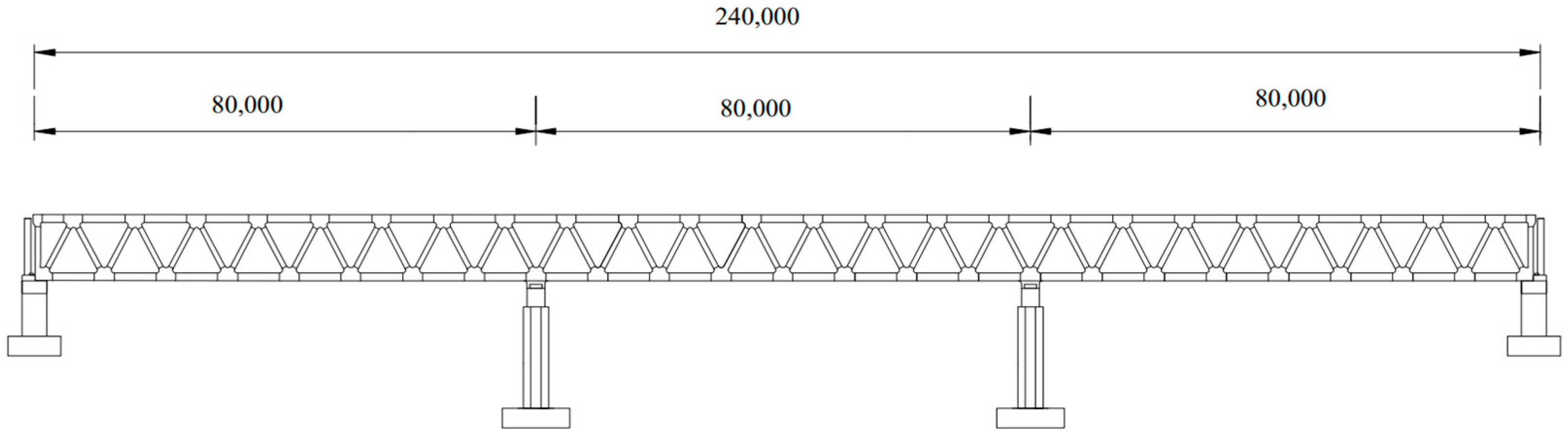
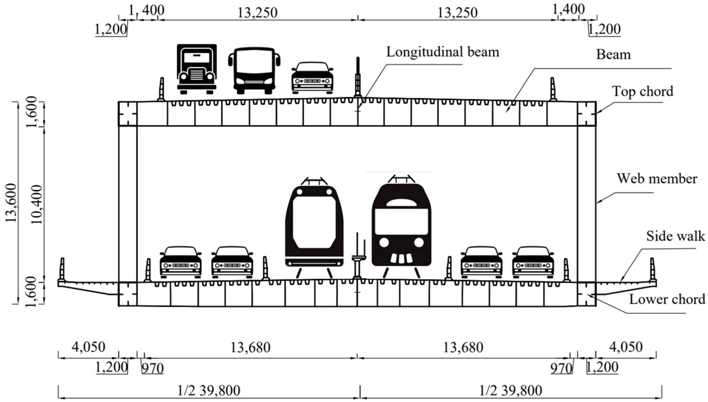
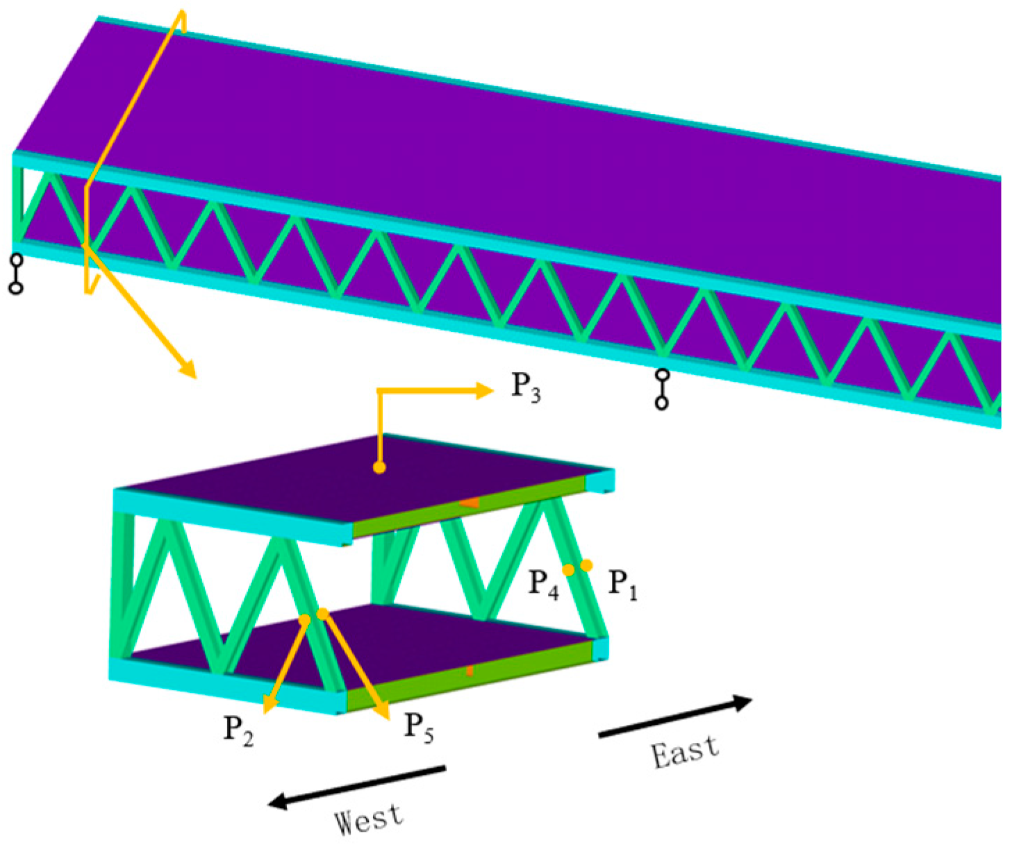
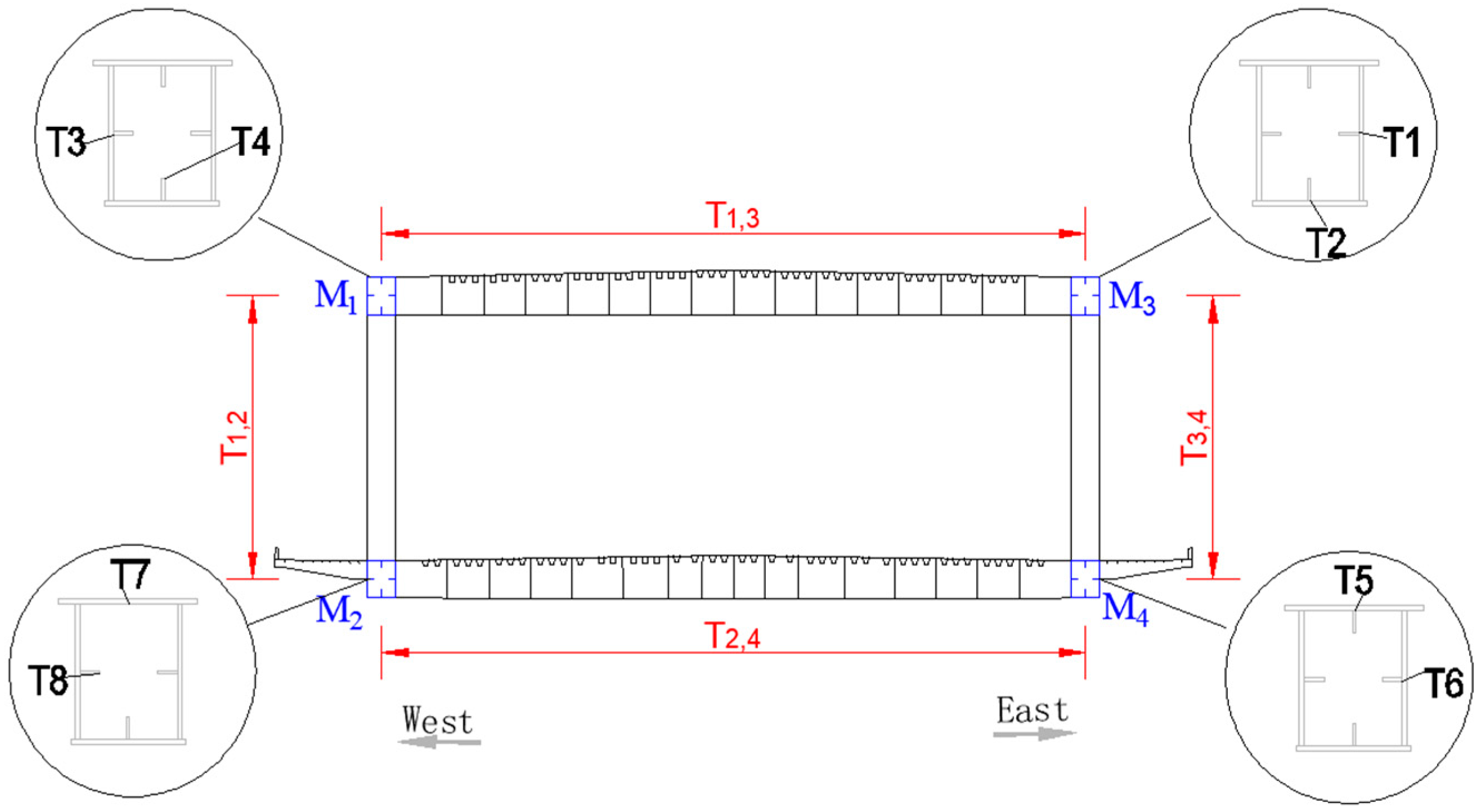
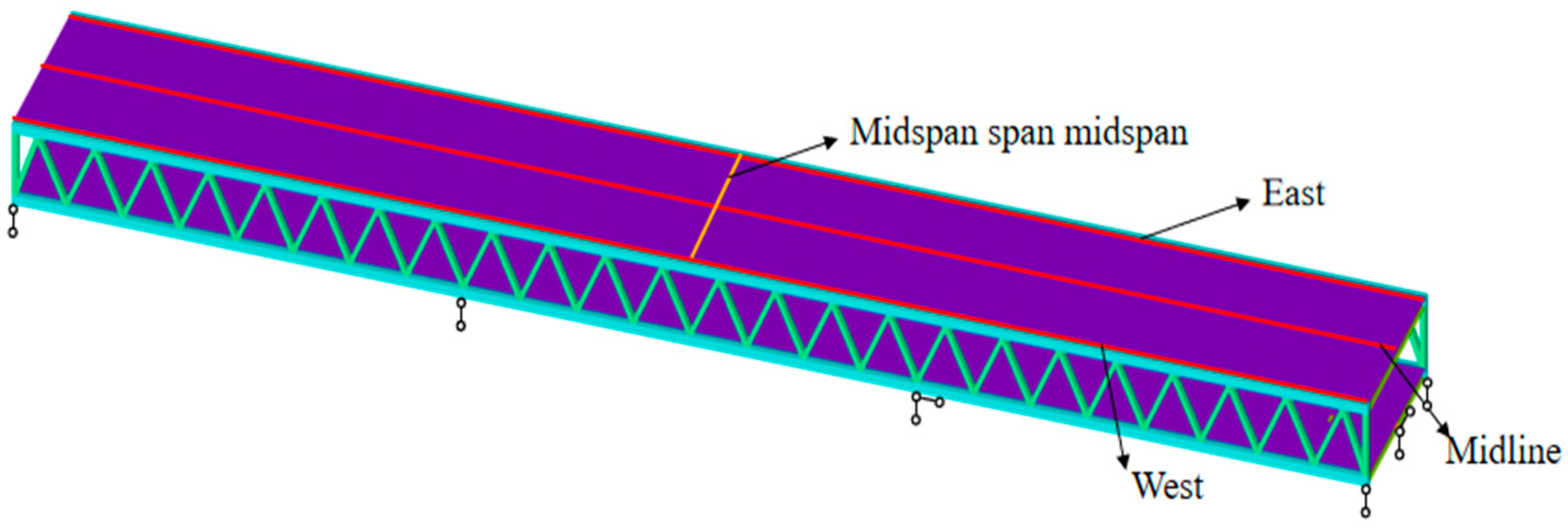
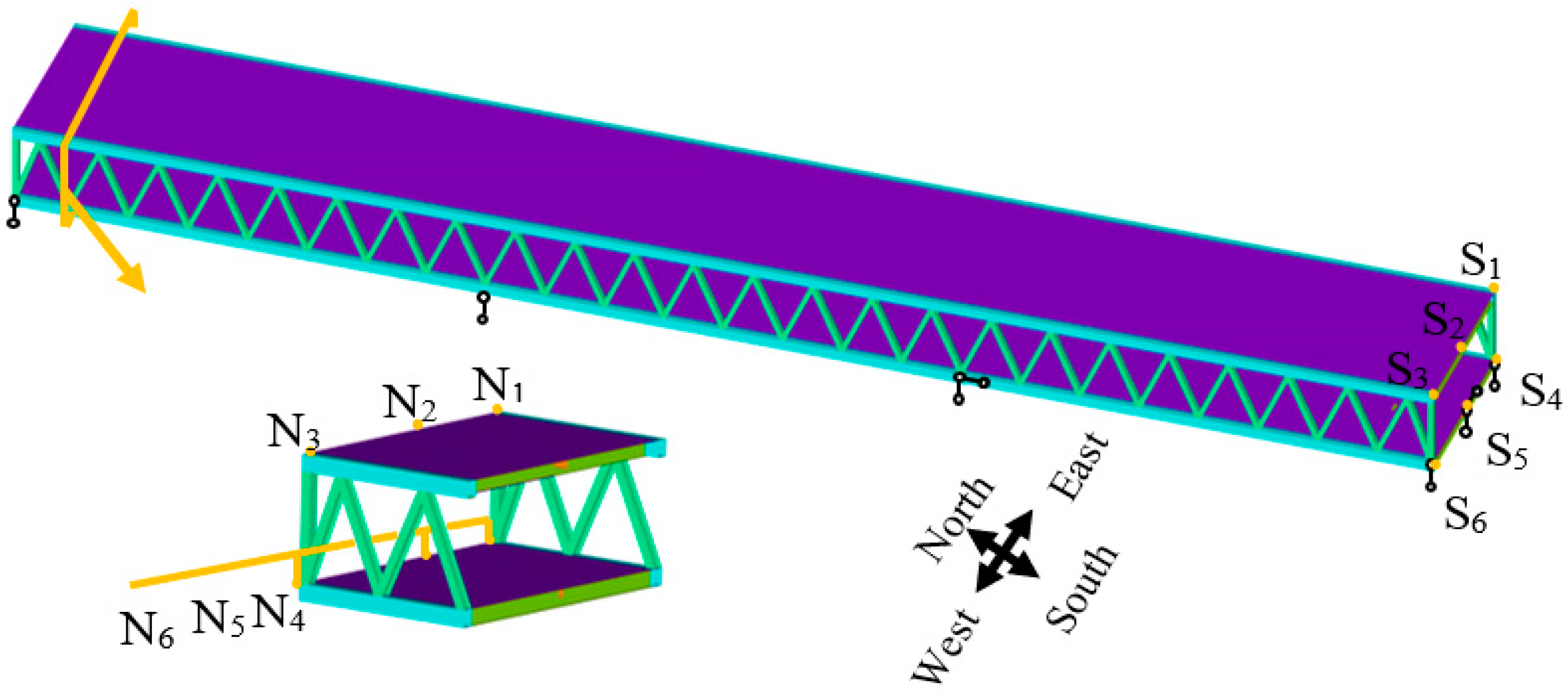
2.5.1. Selection of Research Subjects

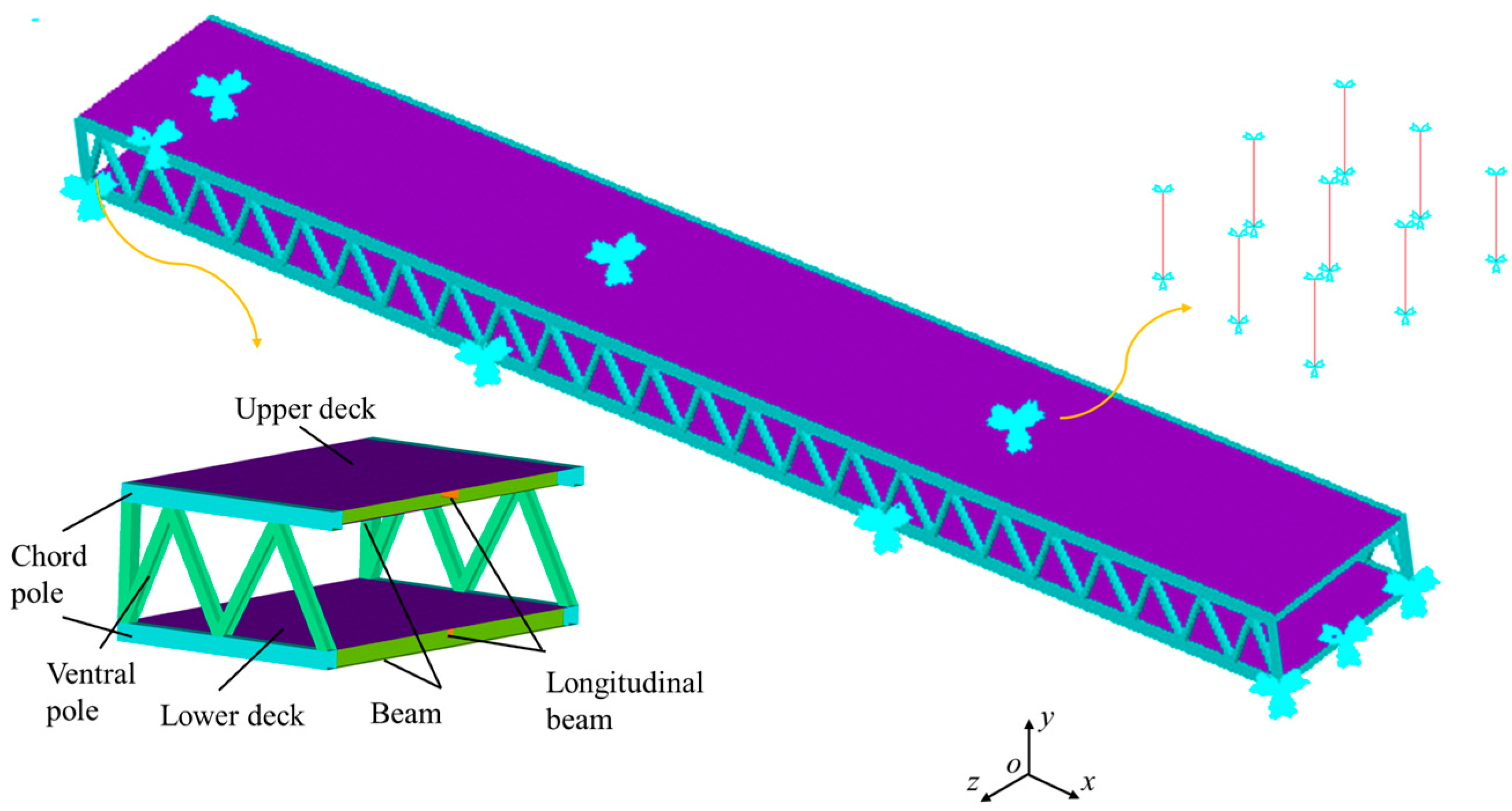
The research focuses on a double-layer steel truss continuous girder, which consists of a 3 × 80 m steel truss continuous girder with separate layers for highway and railway purposes, as illustrated in Figure 4. The primary truss is designed as a triangular structure with a center spacing of 30.5 m and a truss height of 12 m. Both the upper and lower chords of the main truss are box-shaped sections with dimensions of 1200 mm (width) and 1600 mm (height), and with a plate thickness of 30 mm. The diagonal web members adopt an I-shaped section, while the straight web members utilize a box-shaped section measuring 1200 mm (width) and 1000 mm (height), and having a plate thickness of 36 mm. For the upper and lower bridge decks, they consist of cross beams, longitudinal beams, and orthotropic bridge decks. All cross beams and longitudinal beams are inverted T-shaped sections with respective heights of 1600 mm (cross beam) and 800 mm (longitudinal beam). Additionally, the wing plates have widths measuring 720 mm (cross beam) and 400 mm (longitudinal beam), as depicted in Figure 5.

The material of the steel truss is Q370qE, with a yield strength f_y = 430 MPa and ultimate strength f_u = 582 MPa. The material parameters of Q370qE are shown in

Table 2. Q370qE material parameters.

Q370qE	Numeric Value
Mass density ρ	7850 kg/m3
Thermal expansion coefficient α	1.2 × 10−5 °C−1
Poisson’s ratio υ	0.31
Specific heat capacity c	434 J/kg·°C
Isotropic thermal conductivity	60.5 W/(m·°C)
Elastic modulus E	2.06 × 105 MPa

[30,31].

2.5.2. Modeling

An advanced simulation model of a three-span double-layer steel truss continuous girder is established using the general-purpose finite element software ANSYS 2021. To improve both the accuracy and computational efficiency of the temperature analysis, the SHELL131 element is utilized. This element consists of four nodes, each node capable of handling up to 32 temperature degrees of freedom, making it well-suited for three-dimensional steady-state or transient analysis. In contrast, for structural analysis, the SHELL181 element is employed, characterized by its four nodes, where each node has six degrees of freedom. The simulation model of the double-layer steel truss continuous girder is illustrated in Figure 6, whereas Figure 7 presents the mechanical boundary conditions of the simulation model.

The model is simplified in two ways. Firstly, the calculation of the sidewalk slab is disregarded in the model analysis. However, its shielding effect on the bottom chord cannot be overlooked. As depicted in Figure 8, there is minimal disparity observed in the vertical displacement of the structure before and after simplifying the sidewalk board. Secondly, to account for the frame effect of a double-layer bridge deck, an equivalent thickness is assigned to simplify the U-shaped bridge deck as an equally thick bridge deck. The formula used for calculating this equal plate thickness is:

$$t_w=\frac{\mathrm{abE}{A}_c}{2G{\left(\frac{a^2}{4}+b^2\right)}^{3/2}}+\frac{24E{I}_a{I}_b}{Gab\left(a{I}_b+b{I}_a\right)}$$

(12)

where a, b, c (h) represent the spacing between nodes, the height between nodes, and the length of the diagonal web member, respectively, as shown in Figure 9; I_i (m⁴) is the in-plane bending moment of inertia of each member; A_c (m²) is the cross-section area of the diagonal web; E (N/m²) is the elastic modulus; and G (N/m²) is the Shear modulus.

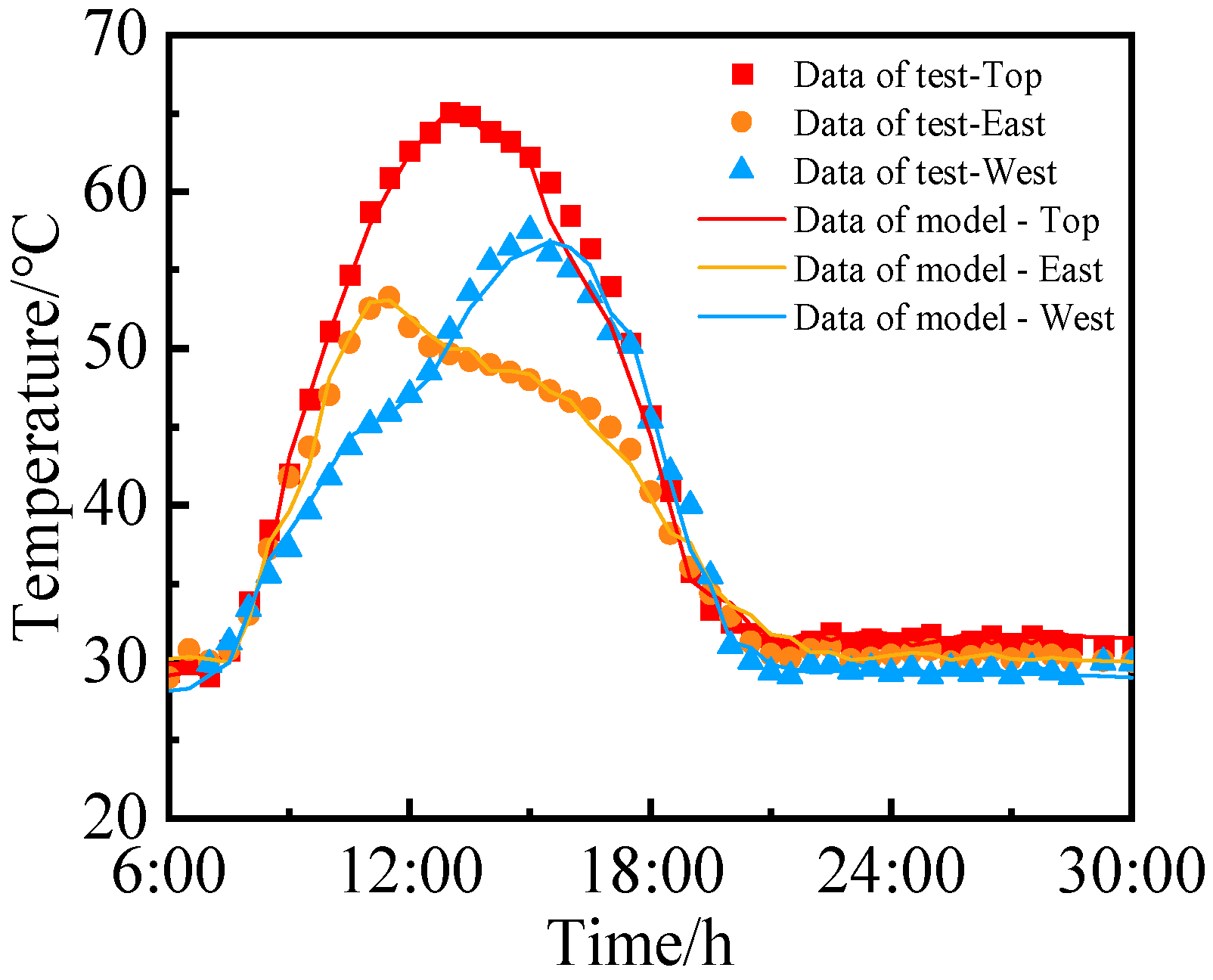
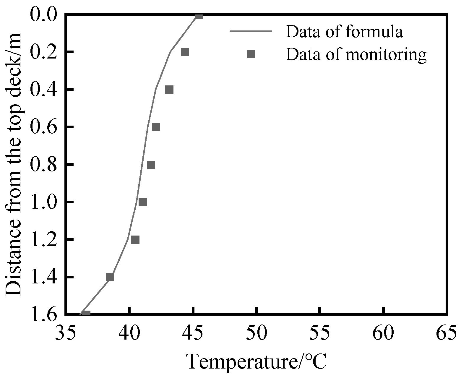
2.5.3. Temperature Analysis Verification

The test data obtained from the steel box girder segment experiment conducted by Tong was selected to validate the numerical model [32]. The validation results of the temperature analysis are presented in Figure 10. Upon comparing the on-site test data with the finite element simulations, it can be concluded that there is a consistent time point at which the top plate, east side, and west side of the steel box girder reach their maximum temperatures. Furthermore, the difference between these two sets of results is within 2.22%. It is evident that the temperatures predicted by our model exhibit excellent agreement with those measured during testing.

3. Time-Varying Temperature Field

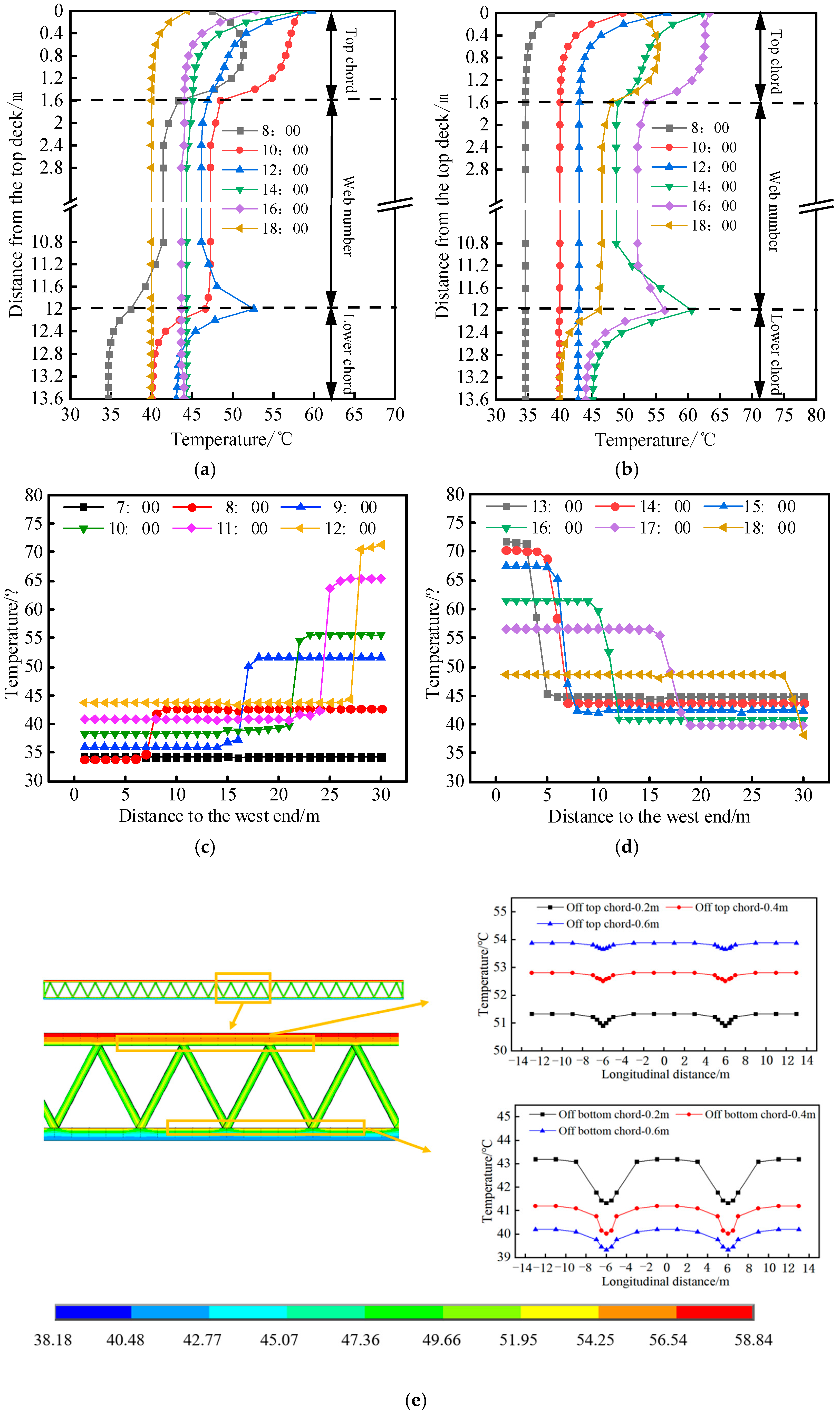
3.1. Time-Varying Temperature Field Distribution Law of The Whole Structure

Due to the time-varying solar radiant intensity and radiation angle, as well as component shielding effects, temperature gradients exist in the vertical, horizontal, and longitudinal directions of the overall steel truss. Moreover, the temperature at different time points within a specific location also varies.

The vertical temperature distribution, as depicted in Figure 11a,b, exhibits an uneven pattern along the east–west direction with a noticeable temperature gradient. Specifically, during the period from 8:00 to 12:00, the eastern region of the steel truss experiences direct sunlight exposure, while, from 14:00 to 18:00, it shifts to the western region. The observed temperature gradient primarily manifests in areas adjacent to the upper chord top plate and side plate, as well as between the upper chord and web, and lower chord and web. The transverse temperature distribution, as depicted in Figure 11c,d, exhibits a discernible correlation between the lower deck’s temperature and the shading effect. Notably, the shaded area experiences significantly lower temperatures compared to the unshielded region, leading to a distinct stepped temperature gradient. At its peak, the lateral temperature difference can reach up to 29.73 °C at 13:00. The temperature in the shaded areas is primarily influenced by the ambient temperature, whereas the temperature in the unshaded areas is predominantly affected by solar radiation. In terms of the longitudinal temperature distribution (as depicted in Figure 11e), apart from the vicinity near the connections of chord and web members, the temperatures at each point along the same height of the steel truss are equivalent. A slight temperature gradient exists near the connection points of the steel truss. Near the bottom chord, the longitudinal temperature difference decreases as the distance from the bottom chord increases. Similarly, near the top chord, the longitudinal temperature difference diminishes with increasing distance from the top chord. Based on the data comparison, it is evident that heat transfer in the connection area is more significantly influenced by the lower chord than by the upper chord.

To further investigate the time-varying temperature law of the entire structure, five characteristic points were selected for temperature analysis. The position and temperature change pattern of these characteristic points are illustrated in Figure 12 and Figure 13, respectively. Figure 12 shows that characteristic point P1, situated on the outer side of the web member, experiences a rapid increase in temperature between 6:00 and 10:00, reaching a maximum value of 54.15 °C at 10:00, followed by a subsequent decrease in temperature. Characteristic point P2, located on the outer side of the western web member, exhibits a gradual warming trend between 6:00 and 10:00, primarily influenced by environmental temperatures. However, during the period from 12:00 to 16:00, it undergoes a significant rise in temperature due to the solar radiation impact with a peak value of 60.91 °C observed at 16:00. The upper bridge level’s characteristic point P3 demonstrates continuous and rapid heating since 6:00 until reaching its maximum value of 71.21 °C at 13:00. Thereafter, the temperature decreases as the radiant intensity diminishes. Feature points P4 and P5 are positioned on the inner side of both eastern and western web members, respectively. Their respective temperature changes exhibit overall gentleness, mainly affected by environmental temperatures. However, a notable increase in the heating rate is observed near 18:00 and 8:00 under direct sunlight exposure. From these observations, it can be concluded that solar radiation significantly impacts surface temperatures across this structural system.

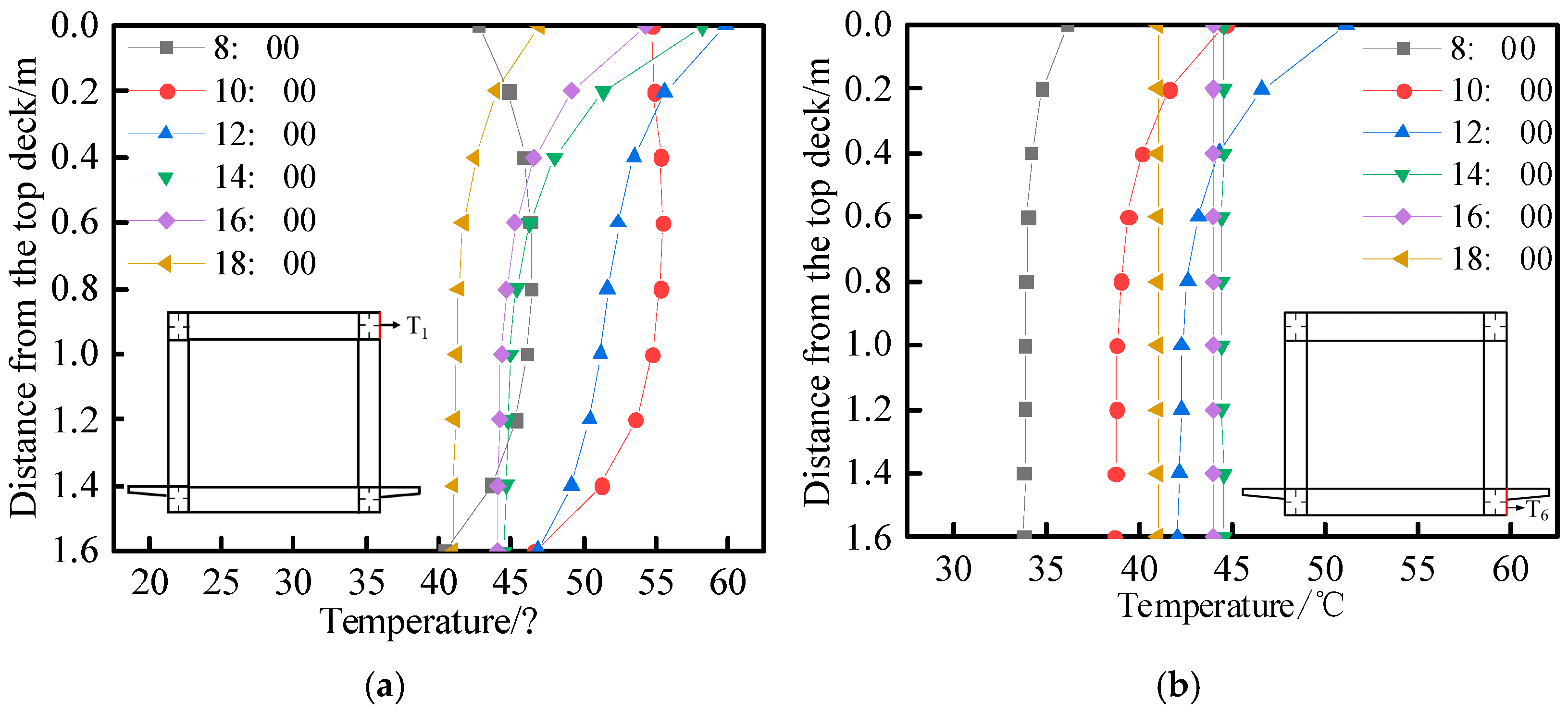
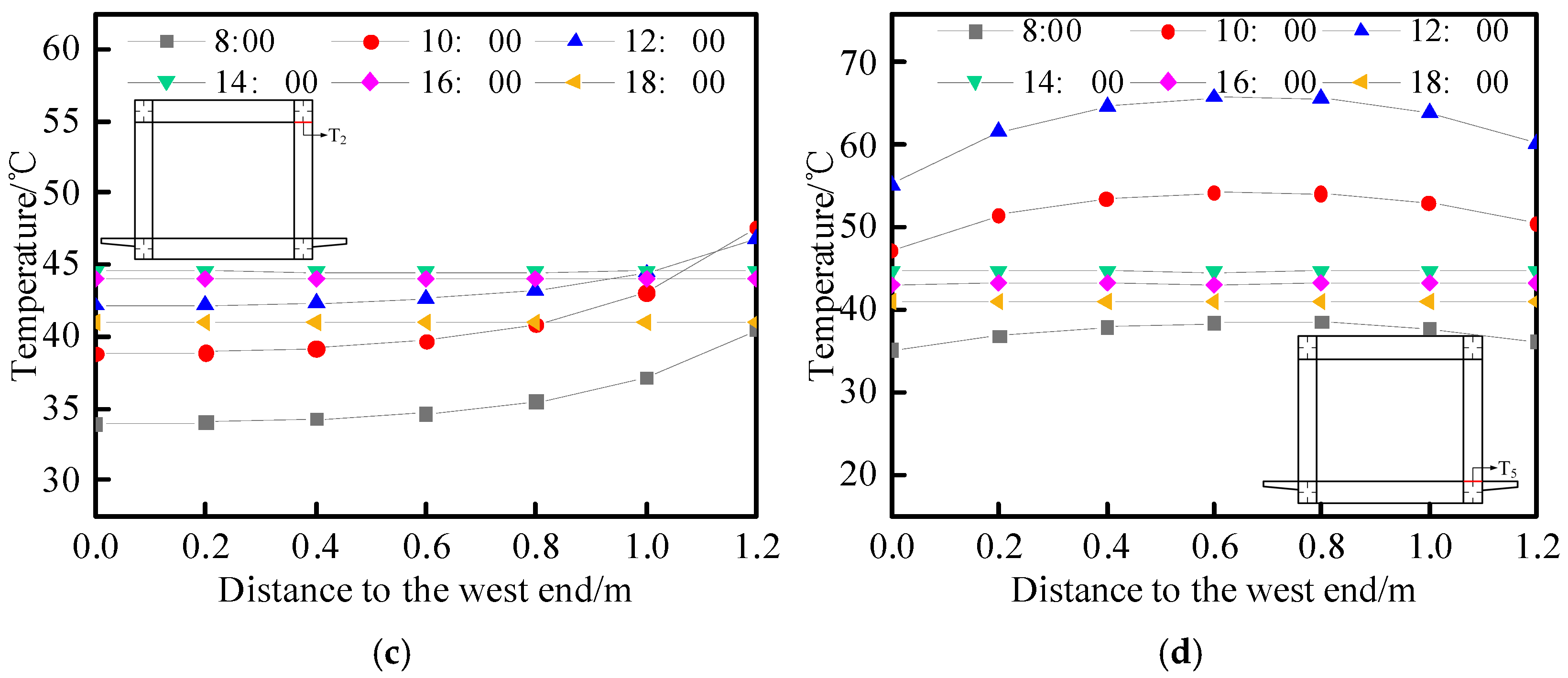
3.2. Temperature Distribution Model of Chord Section

The analysis objects consist of eight typical sections (T1–T8), as illustrated in Figure 14. A detailed examination was conducted on the temperature distribution patterns at the interfaces to investigate the underlying mechanisms governing temperature gradients within chord sections under both sunlight and shading conditions. Taking the eastern side of the steel truss as an example, depicted in Figure 15, it can be observed that T1 and T6 predominantly exhibit “J-shaped,” “convex,” and “S-shaped” temperature gradient profiles. On the other hand, lateral plates T2 and T5 primarily display temperature gradient modes characterized by a “middle convex”, “right convex”, or a single type pattern. It is worth noting that solar radiation angles significantly influence these temperature gradient modes, resulting in varying temperatures between the side plates and either the bottom or top plates due to differences in the solar radiant intensity. Consequently, this leads to distinct heat transfer processes and, subsequently, generates diverse temperature distribution lines.

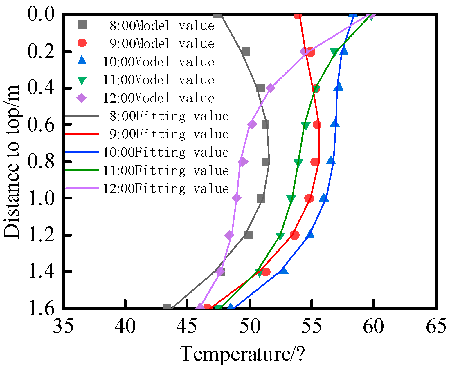
3.3. Distribution Law of Time-Varying Temperature Field on Double Deck

The temperature distribution pattern of the upper deck remains have selected the temperature distribution of the bridge deck at 12:00 as an illustrative example. Figure 16 depicts the grid-like temperature distribution across the entire upper deck. Due to heat transfer effects, the bridge deck will conduct heat transfer like low-temperature longitudinal beams, cross beams, and chords, resulting in a temperature gradient and a grid-like temperature distribution on the bridge deck. The temperature difference between regions L₁ and L₂ is smaller than that within region L₂, indicating a more rapid temperature change in region L₂.

In the sunshine area, the temperature distribution of the lower and upper layers is the same grid distribution, as shown in Figure 17. In the shaded area, the temperature on the bridge deck is evenly distributed and significantly lower than in the sunlight area, and there is a clear temperature boundary between the two regions. In addition, the temperature dividing line moves with the change of the solar zenith angle. At 12:00, the lower bridge deck is completely covered, the overall temperature is evenly distributed, and the small area in the east is grid-distributed.

The temperature distribution in the sunshine area exhibits a uniform grid pattern for both the lower and upper layers, as depicted in Figure 17. Conversely, within the shaded region, the temperature on the bridge deck demonstrates an even distribution that is significantly lower compared to the sunny area, with a distinct thermal boundary separating these two regions. Furthermore, this temperature demarcation line shifts correspondingly with variations in the solar zenith angle. At noon, when the lower bridge deck is completely shielded from direct sunlight, an overall homogeneous temperature distribution prevails while a small eastern section maintains a grid-like pattern.

3.4. Calculation Formula of Temperature Gradient of Component Section

3.4.1. Proposed Formula

We utilize MATLAB 2021 to fit the temperature gradient formulae of each cross-section and, subsequently, derive the time-dependent function of gradient parameters. Considering the identical temperature distribution patterns on both the east and west sides of the double-layer steel truss, as well as the similarity in the fitting procedures for different time points of the component sections, we select the upper chord section at 8:00 as a representative case for calculating the temperature gradient formula. The objective function is defined as a cubic polynomial with the following expression:

$$y=a{x}^3+b{x}^2+cx+d$$

(13)

where x is the distance from the top, and y is the temperature value.

We calculate the values of each parameter using the minimum Q in Formula (14):

$$Q={\displaystyle \sum }_{i=1}^n\left(\mathrm{a}{x}_i{}^3+b{x}_i{}^2+c{x}_i+d-y_i\right)$$

(14)

The ultimate fitting formula is $y=-2.84x^3-2.49x^2+8.72x+4.36$. The fitting diagram of the temperature gradient of the upper chord at each time point in the morning is shown in Figure 18, demonstrating a remarkable level of accuracy in the temperature fitting for every time point.

Similarly, we fit the remaining sections to obtain the temperature gradient parameters a, b, c, and d for each section. Once all the parameters are obtained, we establish the functional relationship between them and time to derive the temperature gradient formula for each cross-section at any given time.

Table 3. Formula for temperature gradient of component cross-section.

Component Cross-Section	Formula
Top chord section	$\left\{\begin{array}{l}a=-0.0042t^4+0.21t^3-3.63t^2+24.15t-53.85\\ b=0.034t^4-1.79t^3-33.59t^2-259.42t-704.34\\ c=-0.047t^4+2.52t^3-47.71t^2+375.08t-1037.31\\ d=-0.0092t^4-0.51t^3-10.88t^2-103.81t-309.65\end{array}\right.$
Bottom chord section	$\left\{\begin{array}{l}a=0.15t^4-6.08t^3+90.08t^2-590.31t+1443.31\\ b=-0.51t^4+20.51t^3-303.73t^2-1990.4t-4866.54\\ c=0.56t^4-22.51t^3+333.11t^2-2182.93t-5337.25\\ d=-0.21t^4+8.26t^3-122.32t^2+801.48t-1959.67\end{array}\right.$
Cross beam section	$\left\{\begin{array}{l}a=-0.0056t^4+0.28t^3-4.84t^2+32.05t-71.87\\ b=0.019t^4-0.96t^3+16.47t^2-108.91t+244.19\\ c=-0.021t^4+1.06t^3-18.28t^2+120.88t-271.08\\ d=-0.0079t^4-0.39t^3+6.81t^2+45.01t-100.91\end{array}\right.$
Box-shaped web member	$\left\{\begin{array}{l}a=0.037t^4-1.48t^3+21.14t^2-128.77t-294.41\\ b=-0.034t^4+1.36t^3-19.51t^2+119.56t-275.05\\ c=0.014t^4-0.57t^3+8.24t^2-51.11t+118.86\\ d=-0.0002t^4+0.0082t^3-0.12t^2+0.69t-1.57\end{array}\right.$
I-shaped web member	$\left\{\begin{array}{l}a=-0.049t^4-1.94t^3+27.61t^2-168.08t-384.15\\ b=-0.042t^4+1.66t^3-23.61t^2+143.75t-328.56\\ c=-0.015t^4-0.61t^3+8.54t^2-52.01t+118.90\\ d=-0.0003t^4-0.01t^3-0.16t^2+1.03t-2.35\end{array}\right.$

displays the function of temperature gradient parameters for different components over time. Note that, from 12:00 to 18:00, there is no temperature gradient in the bottom chord, box-shaped web, and I-shaped web sections; therefore, their respective temperature gradient formulae only apply from 8:00 to 12:00.

3.4.2. Formula Validation

The 11:00 temperature data of the upper chord box girder of Chongqing Chaotianmen Bridge was selected to validate the proposed temperature gradient formula in this study [33]. The main truss chord of Chongqing Chaotianmen Bridge is a welded box section, available in two variations, 1200 mm and 1600 mm in width. The section height ranges from 1240 mm to 1840 mm, with a plate thickness varying between 20 mm and 50 mm. The main structural material employed is Q420q steel. Due to the difference in the maximum temperature between the literature [33] and the paper, a reduction coefficient (0.76 is adopted here) needs to be considered when calculating component temperatures. Figure 19 illustrates the comparison of the temperature results, demonstrating that the calculated results in this paper align with the linear temperature gradient observed in [33], with a correlation coefficient (R² = 0.9889), thus confirming the formula’s feasibility.

4. Time-Varying Law of Temperature Response

4.1. Structural Displacement

The bridge structure exhibits a significant structural response under the daily temperature cycle. The displacement of the bridge can be categorized into three components: vertical, horizontal, and longitudinal displacements. To extract displacement data, three representative longitudinal lines are selected: the centerline, east and west lines, and the transverse line in the middle span, as depicted in Figure 20. The vertical displacement is positive in the upward direction and negative in the downward direction. The horizontal displacement is positive towards the east and negative towards the west. The longitudinal displacement is positive outwardly and negative inwardly.

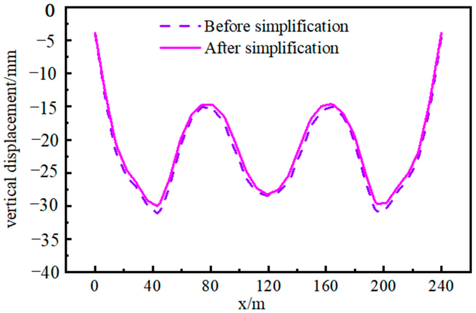
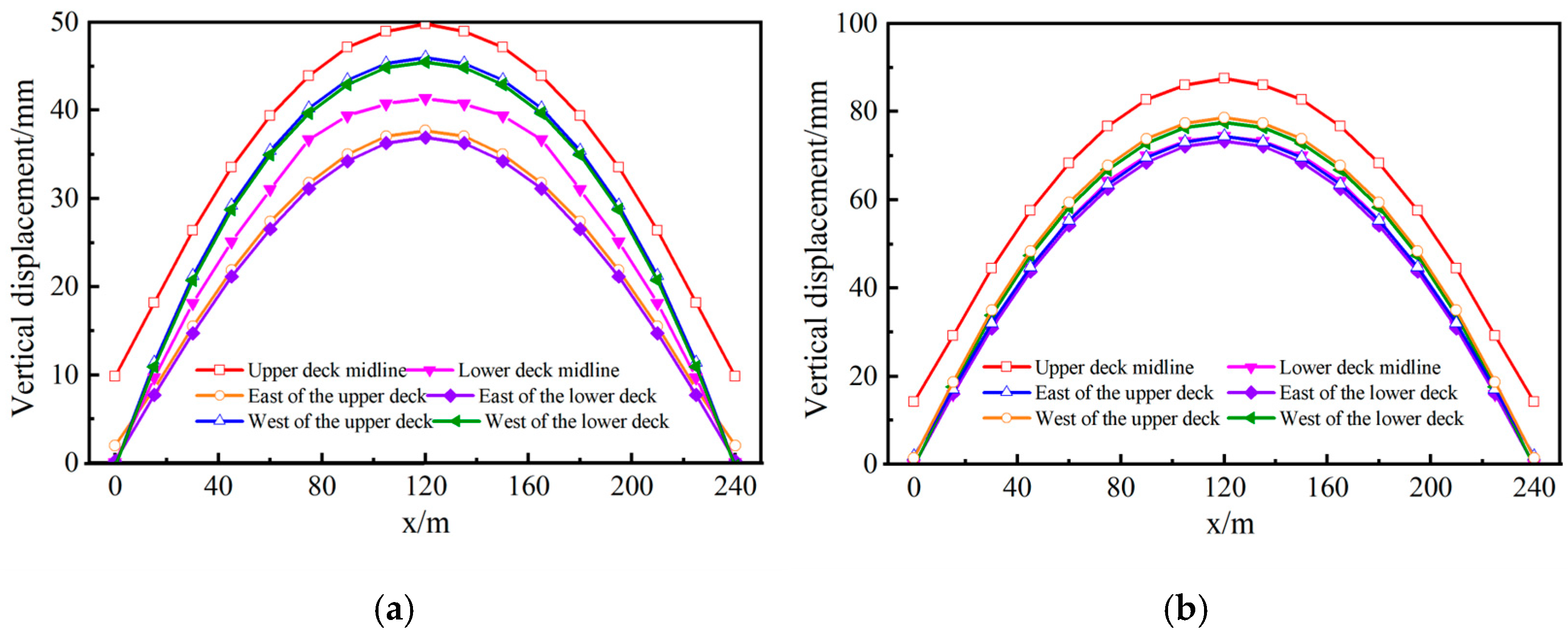
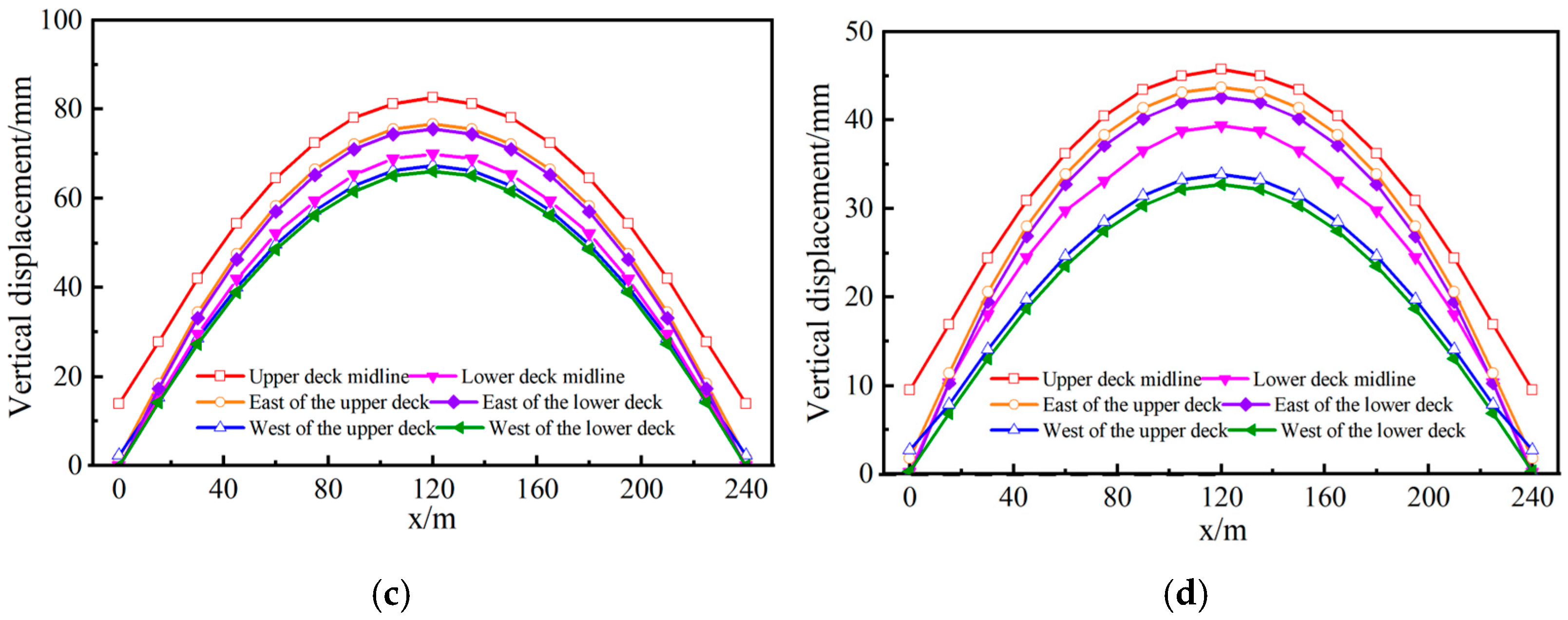
4.1.1. Vertical Displacement

The vertical displacement curve of the double-layer deck at different time points is shown in Figure 21. The vertical displacement of the double-layer deck rises first and then falls during the day, which is positively correlated with the ambient temperature. The vertical displacement distribution pattern of each time point is consistent, and the most significant displacement occurs in the middle span position. The vertical displacement reaches its maximum value at 12:00, with the upper deck measuring 87.69 mm and the lower deck measuring 77.24 mm. The nonuniform lateral temperature distribution of the lower bridge deck due to shading effects necessitates attention to the vertical displacement in the west sides of both the upper and lower decks during design and maintenance.

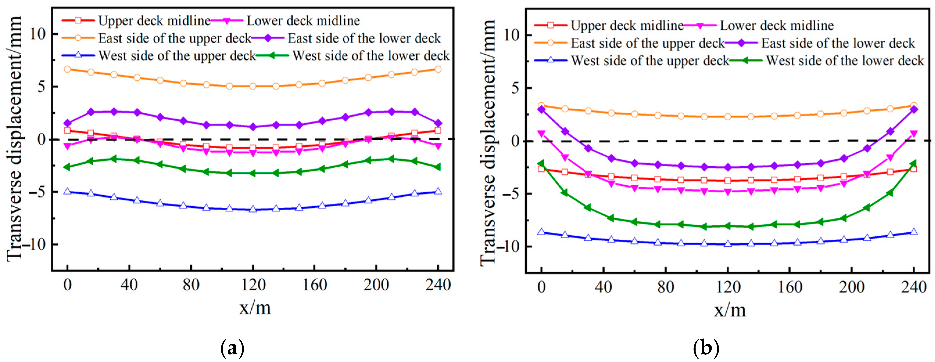
4.1.2. Transverse Displacement

Under the combined influence of the solar radiation angle and support constraints, the position of the maximum lateral displacement changes, as illustrated in Figure 22. Both sides of the upper deck are horizontally offset, while, in the middle span, the lower deck is horizontally offset to both sides and curved to both sides in the side span. There are differences in the distribution patterns of lateral displacement between them. Under the solar radiation influence, the bridge deck temperature rises and expands outward. The direction of the lateral deviation of the center line is determined by the side of the steel truss with a high solar radiation intensity.

4.1.3. Longitudinal Displacement

The end of the continuous girder was marked by selecting twelve specific points, as illustrated in Figure 23. The time-varying curves depicting longitudinal displacement at each of these points under extremely high temperatures are presented in Figure 24a,b. The comparison reveals a consistent changing trend between the south and north ends of the girder. Notably, the outward elongation value at the northern end surpasses that at the southern end. The time variation curve of the longitudinal displacement of the point is analyzed by taking the north end of the continuous girder as an example. For the upper deck, the longitudinal displacements of N₁, N₂, and N₃ are consistent. Under solar radiation, each point is heated and expanded, reaching a maximum of 54.14 mm at 14:00 and then entering the descending stage; for the lower bridge deck, the longitudinal displacements of N₄, N₅, and N₆ are consistent during 6:00~8:00. After 8:00, affected by the angle of solar radiation and shading, the degree of thermal expansion of the three positions was different. The girder end exhibits a complex structural configuration and experiences intricate stress states.

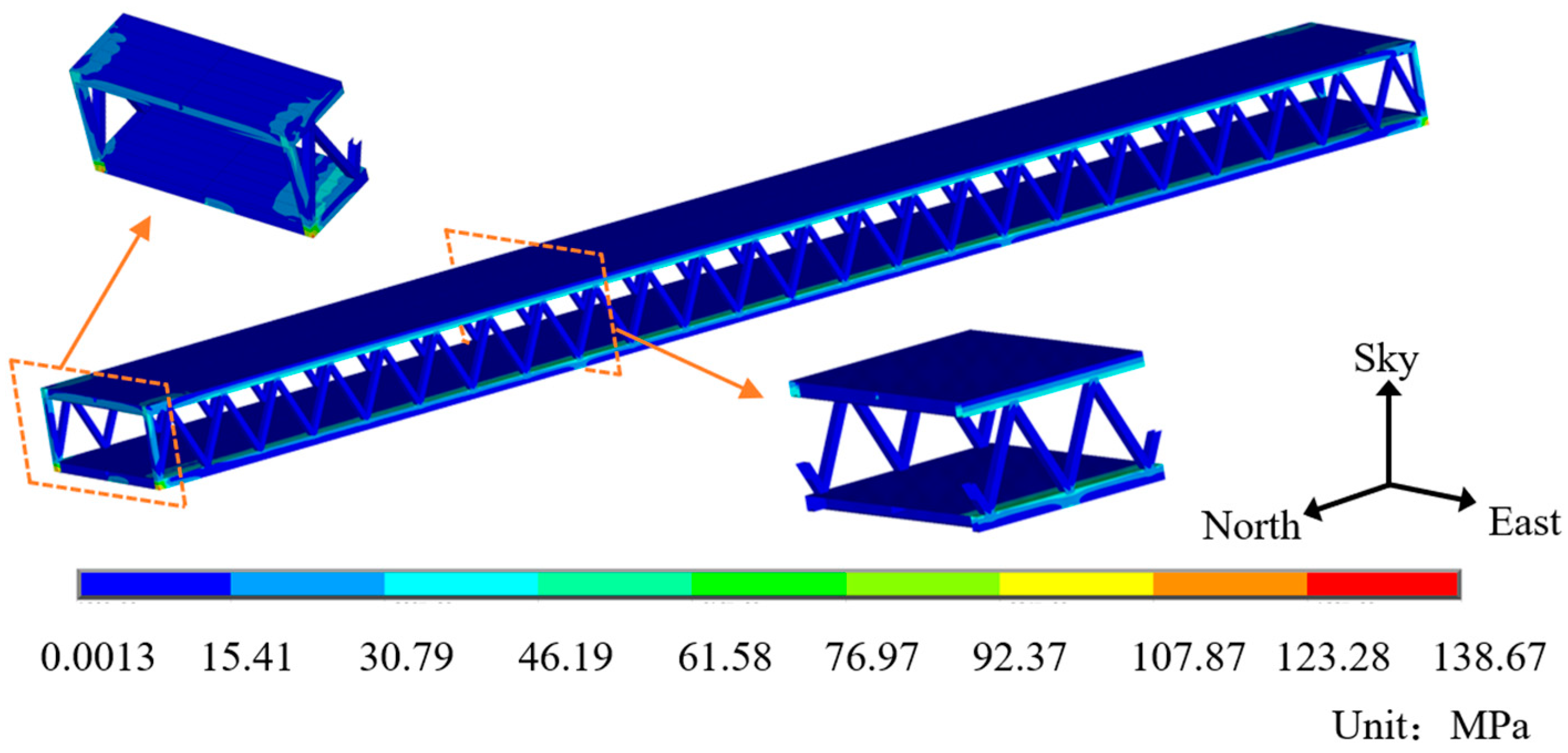
4.2. Structural Stress

The stress utilized in this model refers to the von Mises stress, as defined by the fourth strength theory of elastic–plastic mechanics. As can be seen from Figure 25, the stress predominantly concentrates near the bearing region. Hence, the chord stress at the edge fulcrum section ((4) pier), middle fulcrum section ((3) pier), and fulcrum are selected for analysis.

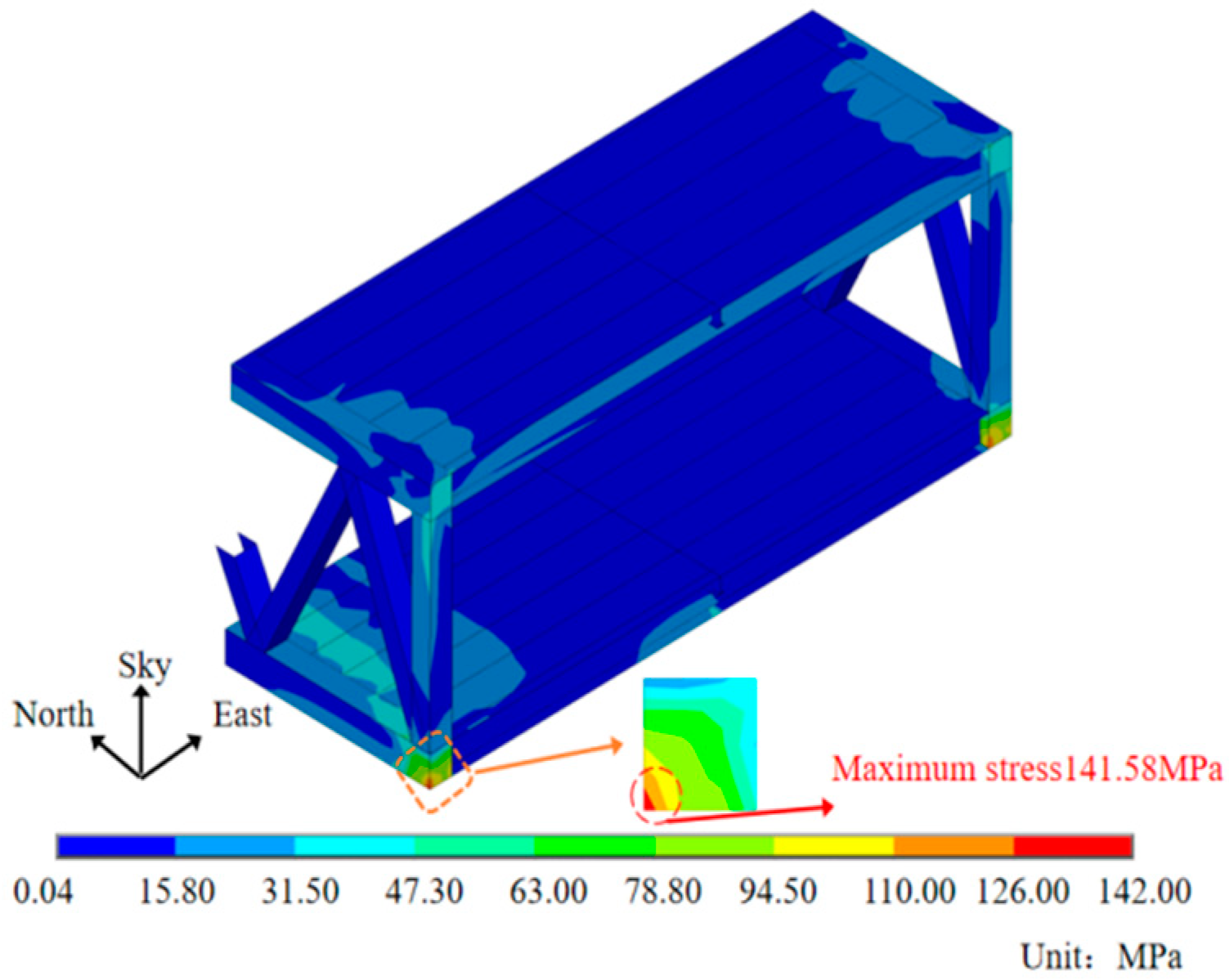
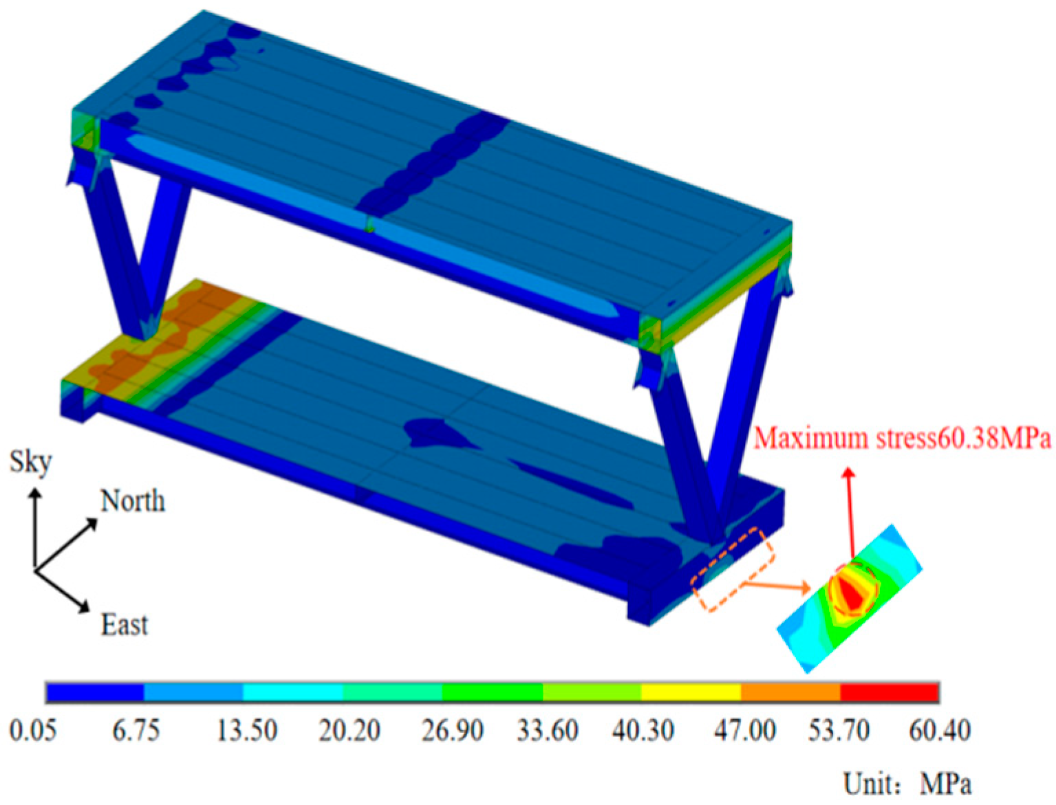
4.2.1. Stress of the Support Sections

The stress distribution of the edge support and middle support sections under the action of all-day sunlight are shown in Figure 26 and Figure 27, respectively. The comparative analysis reveals that the shading effect of the component induces an uneven temperature field, leading to varying degrees of thermal expansion in the steel truss. Consequently, this phenomenon significantly impacts the distribution of stress. The trend of maximum stress variation is the same for the edge fulcrum and middle support section. The stress of the edge fulcrum and the middle fulcrum section were maximized at 14:00, which were 141.48 MPa and 60.38 MPa, respectively. The maximum stress of the edge support section exceeds that of the middle support section at each point.

4.2.2. Stress of Chords

The stress distribution of the chords under solar radiation is primarily concentrated near the supports. Therefore, the stress of the east upper chord, west upper chord, east lower chord, and west lower chord near the supports are extracted, as shown in

Table 4. Stress of chord rod at support section (unit: MPa).

	Location	7:00	10:00	12:00	14:00	16:00	19:00
East-side upper chord	① pier	14.95	38.25	44.18	43.12	28.45	4.02
	② pier	11.64	32.61	42.49	41.93	28.41	1.10
	③ pier	11.60	32.21	42.05	41.98	29.49	1.14
	④ pier	14.99	39.61	44.28	43.42	28.79	3.86
West-side upper chord	① pier	6.57	31.75	44.71	45.75	35.65	8.86
	② pier	2.80	30.69	43.64	44.71	32.30	8.52
	③ pier	2.86	30.68	43.94	44.12	32.55	8.37
	④ pier	6.37	31.59	43.86	45.99	35.53	8.77
East-side lower chord	① pier	10.41	55.38	84.88	80.13	51.65	4.86
	② pier	14.69	29.52	35.91	40.89	38.90	24.62
	③ pier	17.85	32.85	43.96	45.38	40.78	33.94
	④ pier	10.31	55.91	83.84	81.34	52.53	4.07
West-side lower chord	① pier	5.98	53.74	81.46	85.58	66.84	7.96
	② pier	9.95	24.66	28.15	35.51	26.98	15.76
	③ pier	11.96	30.61	36.07	40.44	34.71	28.80
	④ pier	4.85	52.46	80.22	86.08	67.47	7.91

.

The stress of the upper chord on the east is observed to be significantly higher than that on the west during the time interval of 7:00~12:00, as indicated by Table 4. During 14:00~19:00, the magnitude of stress experienced by the upper chord on the western side is significantly higher compared to that on the eastern side. During 12:00~14:00, there exists a subtle disparity in stress levels between the upper chords situated on both sides. The east and west upper chords have the same stress time-varying law at each support. The stress at each support of the upper chord on the east reaches the maximum stress at 12:00. The stress at each support of the upper chord on the west reaches the maximum stress at 14:00. The stress of the lower chord at pier (1) and pier (4) is mainly affected by the intensity of solar radiation. However, the stress at the positions of pier (2) and pier (3) is mainly affected by the constraints, so the stress of the lower chord on the east side at the position of pier (2) and (3) at each time point is greater than that of the lower chord on the west side.

4.3. Steel Truss Girder Rotation Angles

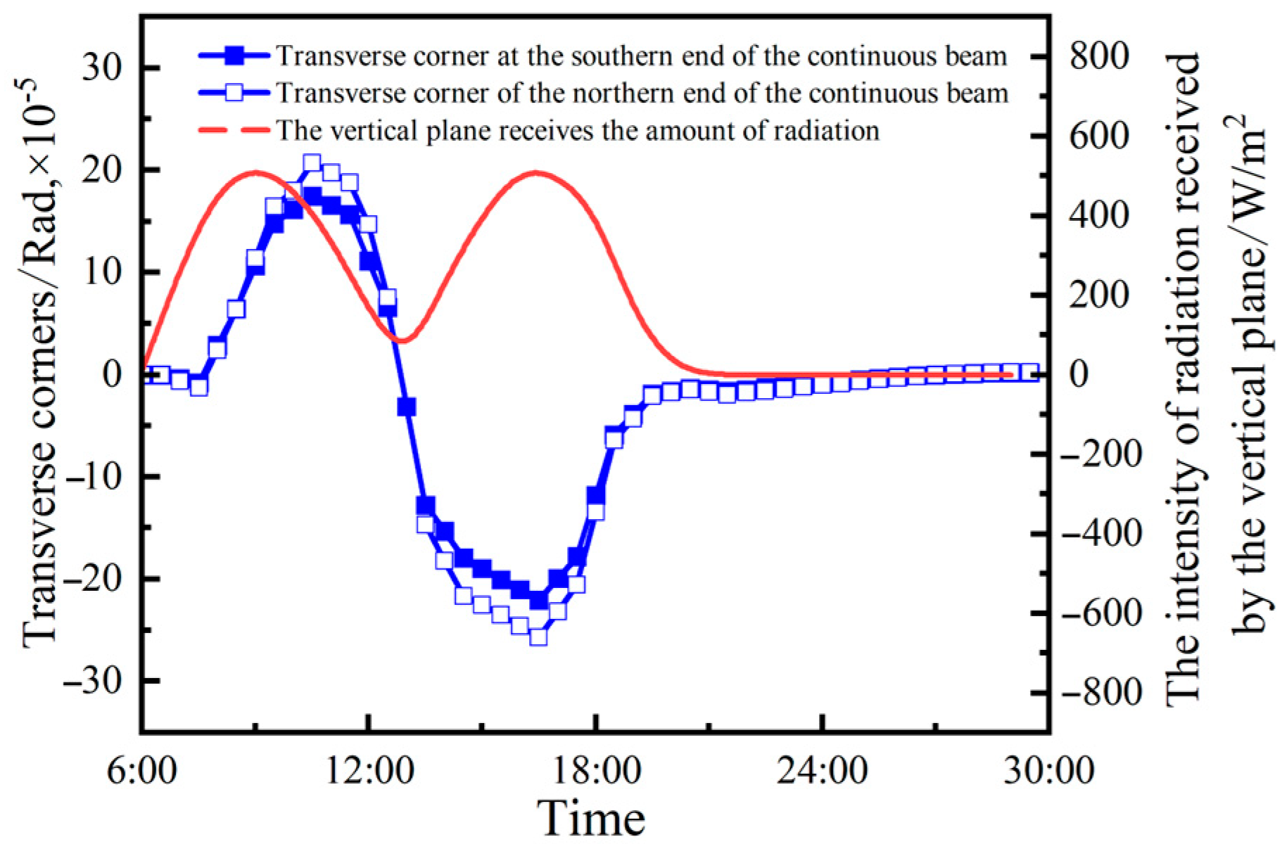
4.3.1. Transverse Rotation Angle of Girder End

The girder end rotation angles encompass both transverse and vertical rotations. The obstruction of the upper bridge on the lower deck results in a significant transverse temperature gradient, induces in-plane bending of the lower deck, and, consequently, leads to substantial transverse rotation angles. Based on the flat-section assumption, it is presumed that, after the deformation of the bridge deck, longitudinal displacements at supports 1, 2, and 3 remain within the plane; support 2 experiences constrained longitudinal displacement while the lateral displacement is considerably smaller than longitudinal displacement. Therefore, the transverse angle can be approximated by the longitudinal displacement of support 1 and support 3, that is:

$$\theta \approx \tan \theta =\frac{H_1-H_3}{D}$$

(15)

The observation of Equation (15) reveals that, as the longitudinal displacement of support 1 surpasses that of support 3, with an increasing difference between them, the lateral angle of the girder end initiates a progressive increment. The lateral rotation angle of the north and south ends of the continuous girder remains relatively stable during nighttime, as depicted in Figure 28. During the period of 10:00~12:00, an increase in the solar radiation angle leads to a gradual reduction in the lateral angle at the girder end. After 12:00, the sun gradually moves towards the west. The longitudinal displacement of support 3 exceeds that of support 1. Additionally, the transverse angle of the girder end becomes negative and reaches its minimum value at 17:00. Subsequently, it gradually approaches zero.

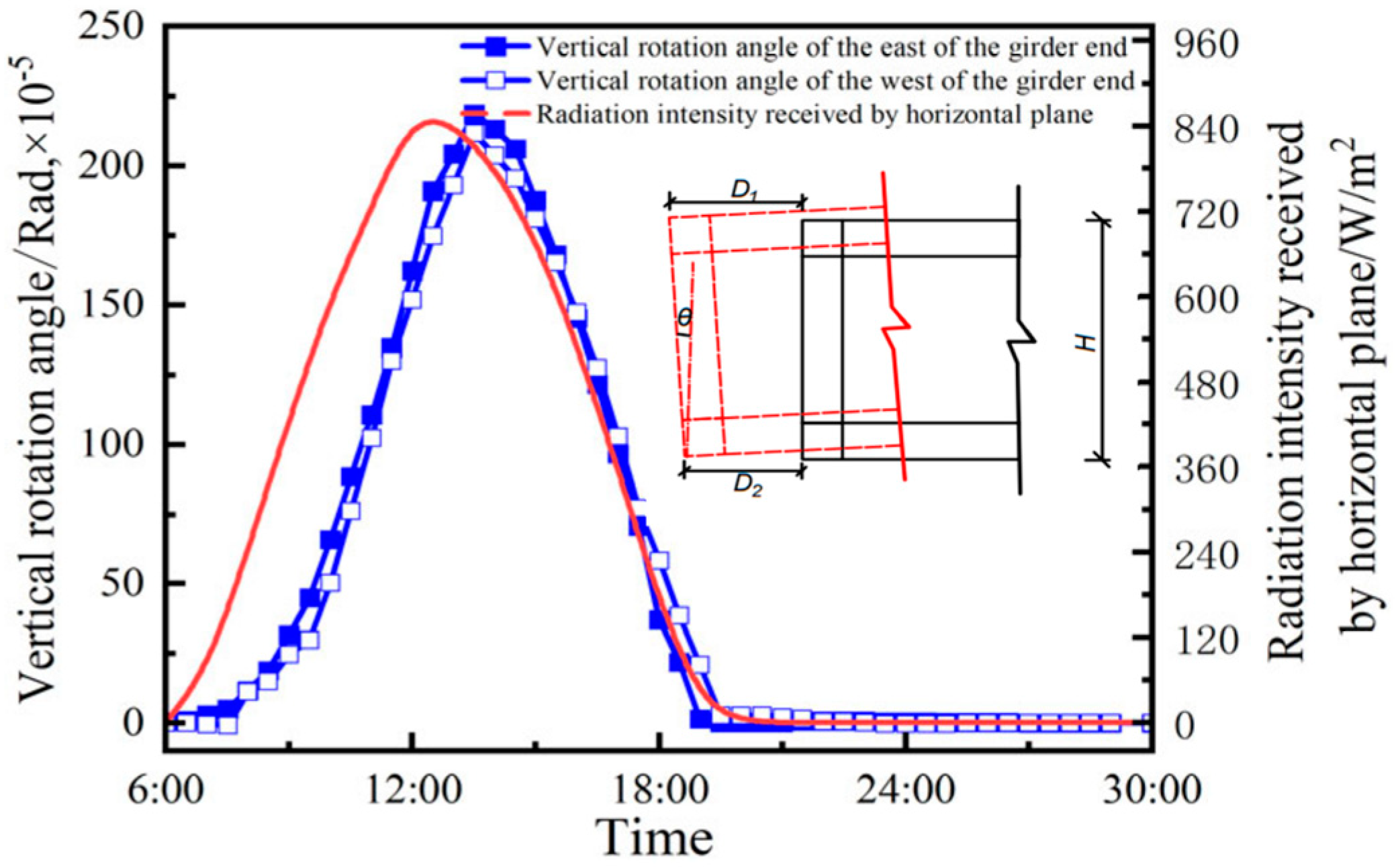
4.3.2. Vertical Rotation Angle of Girder End

Due to the shading effect, the lower bridge deck exhibits a comparatively lower temperature than the upper deck, leading to differential thermal expansion between them and, consequently, resulting in a significant vertical rotation angle of the girder end. The supports on both sides of the girder end are tension–compression support. The vertical displacement is constrained. It can be inferred that the vertical displacement is negligible, while the lateral displacement is significantly smaller than the longitudinal displacement. Therefore, the vertical rotation angle of the girder end can be approximated by the longitudinal displacement of nodes 1 and 2, that is:

$$\theta \approx \tan \theta =\frac{D_1-D_2}{H}$$

(16)

The vertical rotation angle of the girder end is illustrated in Figure 29. The trend of the variation in the vertical rotation angle at both ends of the east and west girders exhibits a high degree of similarity. During the period of 6:00~14:00, the longitudinal displacement of the upper deck’s end exceeds that of the lower deck, while the girder end exhibits a positive and increasing vertical rotation angle, reaching its maximum at 14:00. The limited influence of the double-layer bridge deck’s shielding effect on the vertical rotation angle of the girder end is evident. As a result of reducing the longitudinal displacement difference between the upper and lower deck beam ends, the vertical rotation angle gradually diminishes to zero.

The changing trends and values of the lateral and vertical rotation angles of the girder ends exhibit significant disparities, as evident from Figure 28 and Figure 29, owing to distinct influencing factors governing their variations. The lateral angle of the girder end is primarily determined by the radiation intensity received on the vertical plane, while the vertical rotation angle of the girder end is predominantly influenced by the radiation intensity received on the horizontal plane. The inclination of the girder end increases proportionally with escalating radiation intensity.

5. Conclusions

After investigating the time-varying behavior of the temperature distribution, temperature response characteristics, and structural response of the double-layer steel truss continuous girder under shielding, the following conclusions can be deduced:

• A model analyzing the impact of solar radiation on bridge structures was developed. This model, integrating time-varying thermal boundary conditions and support scenarios, led to an effective temperature analysis framework for the double-layer steel truss continuous girder. Validation efforts revealed that the temperature model’s predictions deviate from experimental data by a mere 2.22%, demonstrating the model’s reliability and effectiveness.
• The study identified distinct vertical, horizontal, and longitudinal temperature gradients within the structure. The vertical gradient, most pronounced on the truss sides, showed a maximum temperature difference of 19.27 °C. The horizontal gradient, concentrated on the lower deck, varied with solar radiation angles, reaching a peak difference of 29.73 °C. The longitudinal gradient, less evident and located at the chord junctions, exhibited a temperature variation within 1.87 °C under solar influence.
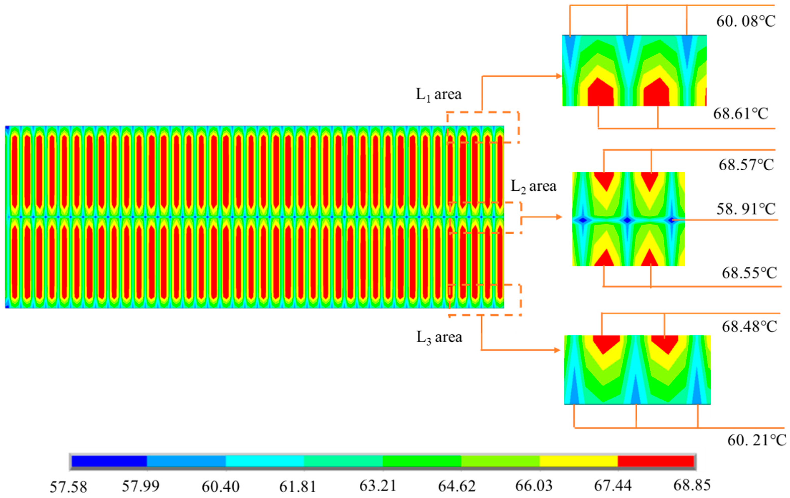
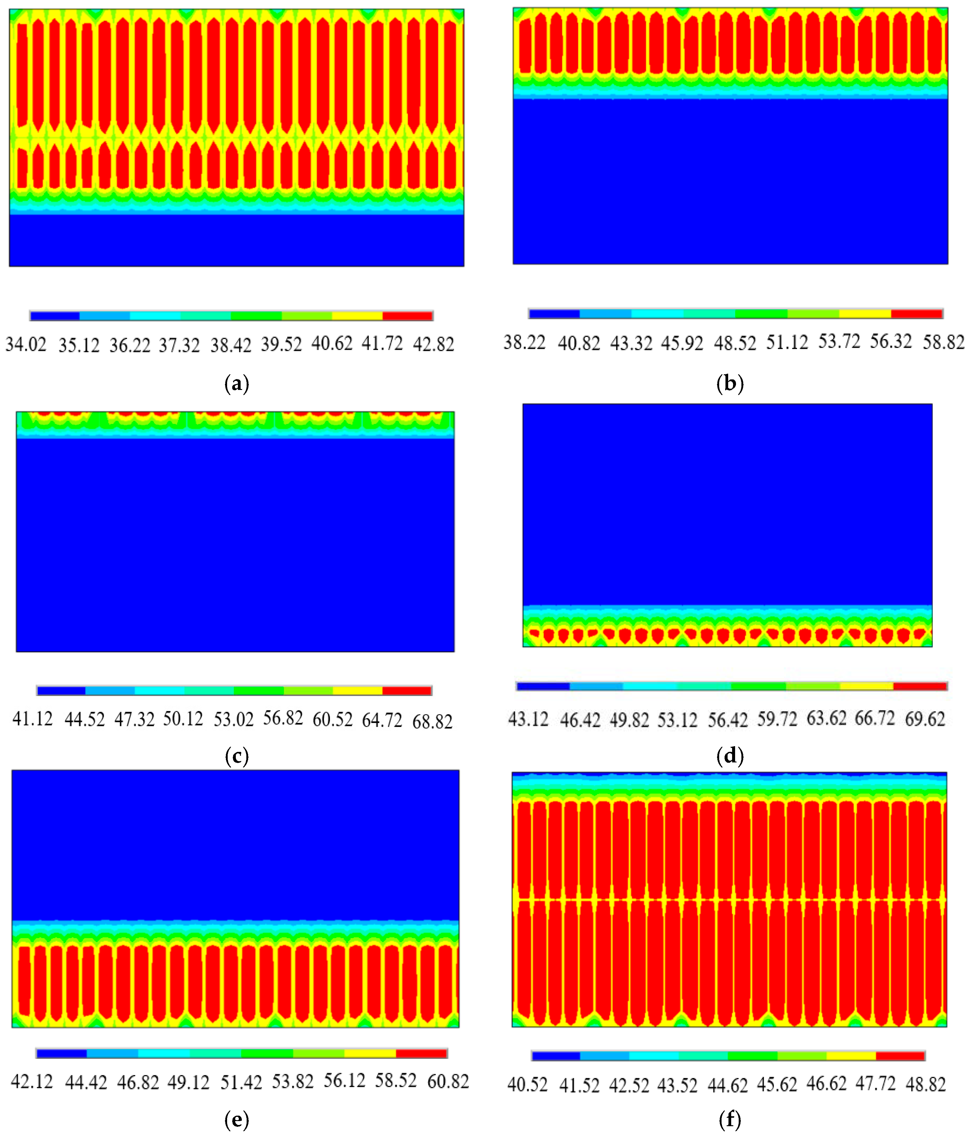
• The proposed temperature distribution model of the chord section under shielding encompasses five vertical temperature gradient distribution models and four horizontal temperature gradient distribution models. These models are primarily influenced by the environmental temperature, solar radiation, and panel heat exchange. A noteworthy finding is the grid-like temperature field distribution in the double deck under shading, with a distinct temperature boundary on the lower deck influenced by the solar altitude angle. Additionally, the study introduces a methodology for determining temperature gradients at any member section time point.
• Shading was observed to significantly influence the displacements of the upper and lower decks, leading to notable disparities. The most considerable vertical displacement difference occurred at noon (22.58 mm), while the lateral and longitudinal displacements showed the maximum differences of 6.50 mm and 7.49 mm, respectively, at different times of day. Uneven transverse temperature distribution was found to alter the maximum stress location in the lateral fulcrum section over time. The study also highlighted that the girder end’s rotational behavior, both transversely and vertically, is subject to the intensity and angle of solar radiation, with a lag in response to radiation intensity changes.

References

1. Xie, X.; Su, H.; Pang, M. Mechanical Properties and Experimental Study of a New Laminated Girder Single Tower Cable-Stayed Bridge. Int. J. Steel Struct. 2023, 23, 872–885. [Google Scholar] [CrossRef]
2. Chen, Y.; Sun, H.; Feng, Z. Study on seismic isolation of long span double deck steel truss continuous girder bridge. Appl. Sci. 2022, 12, 2567. [Google Scholar] [CrossRef]
3. Zhao, Z.; Liu, H.; Chen, Z. Field monitoring and numerical analysis of thermal behavior of large span steel structures under solar radiation. Adv. Steel Constr. 2017, 13, 190–205. [Google Scholar] [CrossRef]
4. Zhu, Q.X.; Wang, H.; Mao, J.X.; Wan, H.P.; Zhang, Y.M. Investigation of temperature effects on steel-truss bridge based on long-term monitoring data: Case study. J. Bridge Eng. 2020, 25, 05020007. [Google Scholar] [CrossRef]
5. Chang, H.; Hu, X.; Ma, R. Numerical study on temperature distribution of steel truss aqueducts under solar radiation. Appl. Sci. 2021, 11, 963. [Google Scholar] [CrossRef]
6. Ozyurt, E.; Wang, Y.C. Effects of truss behavior on critical temperatures of welded steel tubular truss members exposed to uniform fire. Eng. Struct. 2015, 88, 225–240. [Google Scholar] [CrossRef]
7. Liang, J.J.; Liu, L.J.; Zhang, S.S. Temperature field and temperature effect analysis of steel-mixed curved bridge in cold region. Highway 2023, 68, 74–82. [Google Scholar]
8. Zhang, G.; Li, X.Y.; Tang, C.H. Behavior of steel box bridge girders subjected to hydrocarbon fire and bending-torsion coupled loading. Eng. Struct. 2023, 282, 116906. [Google Scholar] [CrossRef]
9. Song, C.; Zhang, G.; Li, X.; Kodur, V. Experimental study on failure mechanism of steel-concrete composite bridge girders under fuel fire exposure. Eng. Struct. 2021, 247, 113230. [Google Scholar] [CrossRef]
10. Fan, J.S.; Liu, C.; Liu, Y.F. Review of temperature field and temperature effect of steel-concrete composite girder bridge. China J. Highw. Transp. 2020, 33, 1–13. [Google Scholar] [CrossRef]
11. Abid, S.R.; Mussa, F.; Tayşi, N.; Özakça, M. Experimental and finite element investigation of temperature distributions in concrete-encased steel girders. Struct. Control Health Monit. 2018, 25, e2042. [Google Scholar] [CrossRef]
12. Wang, R.Z.; Ji, W.; Li, X.T. Thermal load models for the static design of steel-concrete composite girders. Structures 2023, 51, 1004–1018. [Google Scholar] [CrossRef]
13. Wang, G.; Ding, Y. Reliability estimation of horizontal rotation at beam end of long-span continuous truss bridge affected by temperature gradients. J. Perform. Constr. Facil. 2019, 33, 04019061. [Google Scholar] [CrossRef]
14. Wang, Z.; Liu, Y.J.; Tang, Z.W. Three-dimensional temperature field simulation method of truss arch rib based on sunlight shadow recognition. China J. Highw. Transp. 2022, 35, 91–105. [Google Scholar] [CrossRef]
15. Li, Y.; He, S.; Liu, P. Effect of solar temperature field on a sea-crossing cable-stayed bridge tower. Adv. Struct. Eng. 2019, 22, 136943321982864. [Google Scholar] [CrossRef]
16. Wang, G.X.; Ding, Y.L.; Wang, X.J.; Yan, X.; Zhang, Y.F. Long-term temperature monitoring and statistical analysis on the flat steel-box girder of sutong bridge. J. Highw. Transp. Res. Dev. 2014, 8, 63–68. [Google Scholar] [CrossRef]
17. JTG D60-2015; General Code for Highway Bridge and Culvert Design. China Communications Press Co., Ltd.: Beijing, China, 2015.
18. TB 10092-2017; Code for Design of Concrete Structure of Railway Bridge and Culvert. China Railway Press Co., Ltd.: Beijing, China, 2017.
19. EN 1991-1-5:2003; Eurocode1, Actions on Structures, Part1-5: General Actions-Thermal Actions. European Committee for Standardization: Brussels, Belgium, 2003.
20. American Association of State Highway and Transportation Officials, AASHTO. AASHTO LRFD Bridge Design Specifications; American Association of State Highway and Transportation Officials, AASHTO: Washington, DC, USA, 2020. [Google Scholar]
21. Zhu, Y.; Guo, H.; Sun, D.Q. Refined analysis of spatiotemporal heterogeneous temperature field and its effect of sunshine of railway steel truss suspension bridge. Eng. Mech. 2023, 1–13. [Google Scholar]
22. Zhang, H.; Liu, D.Y.; Zhao, W.G.; Ding, S.Y.; Liu, W.; Yang, J.K.; Lu, W.L. Study on temperature field boundary conditions and distribution of steel trusses for public railway dual-purpose use. China Railw. Sci. 2023, 44, 91–101. [Google Scholar]
23. Wang, G.X.; Ding, Y.L. Research on monitoring temperature difference from cross sections of steel truss arch girder of Dashengguan Yangtze Bridge. Int. J. Steel Struct. 2015, 15, 647–660. [Google Scholar] [CrossRef]
24. Wang, G.; Ding, Y.; Liu, X. The monitoring of temperature differences between steel truss members in long-span truss bridges compared with bridge design codes. Adv. Struct. Eng. 2019, 22, 1453–1466. [Google Scholar] [CrossRef]
25. Wang, G.; Zhou, X.; Ding, Y.; Liu, X. Long-term monitoring of temperature differences in a steel truss bridge with two-layer decks compared with bridge codes: Case study. J. Bridge Eng. 2021, 26, 05020013. [Google Scholar] [CrossRef]
26. National Meteorological Information Center. Historical Dataset of Ground Meteorological Observations in China [EB/OL]. Available online: http://data.cma.cn/data/cdcdetail/dataCode/A.0019.0001.S001.html (accessed on 10 March 2023).
27. Zhang, F.; Gao, H.; Cui, X. Frequency of extreme high temperature days in China, 1961–2003. Weather 2008, 63, 30–42. [Google Scholar] [CrossRef]
28. Duffie, J.A.; Beckman, W.A. Solar Engineering of Thermal Processes; John Wiley & Sons: Hoboken, NJ, USA, 2013; pp. 36–65. [Google Scholar]
29. Kim, S.H.; Park, S.J.; Wu, J.; Won, J.H. Temperature variation in steel box girders of cable-stayed bridges during construction. J. Constr. Steel Res. 2015, 112, 80–92. [Google Scholar] [CrossRef]
30. JTG D64-2015; Code for Design of Highway Steel Structure Bridges. China Communications Press: Beijing, China, 2015.
31. Yang, S.M.; Tao, W.Q. Heat Transfer, 4th ed.; Higher Education Press: Beijing, China, 2006. [Google Scholar]
32. Tong, M. Temperature Distribution in Highway Bridges. Master’s Thesis, University of Hong Kong, Hong Kong, China, 2000. [Google Scholar]
33. Duan, F. Research on the Sunshine Temperature Field and Temperature Effects on Long-Span Steel Bridge. Master’s Thesis, University of Southwest Jiaotong, Chengdu, China, 2010. [Google Scholar]
Figure 1. Double-deck shading model.
Buildings 13 02889 g001
Figure 2. Time-varying curve of solar radiation.
Buildings 13 02889 g002
Figure 3. Heat exchange model for continuous steel truss girders.
Buildings 13 02889 g003
Figure 4. Vertical cross-section of double-layer steel truss continuous girder bridge (mm).
Buildings 13 02889 g004
Figure 5. Cross-section of double-layer steel truss continuous girder bridge (mm).
Buildings 13 02889 g005
Figure 6. Advanced simulation model.
Buildings 13 02889 g006
Figure 7. Support layout.
Buildings 13 02889 g007
Figure 8. Vertical displacement comparison.
Buildings 13 02889 g008
Figure 9. Schematic diagram of rod components.
Buildings 13 02889 g009
Figure 10. Validation of the numerical model.
Buildings 13 02889 g010
Figure 11. Longitudinal temperature distribution of steel truss. (a) Vertical distribution temperature of west side. (b) Vertical distribution temperature of east side. (c) Transverse temperature distribution (morning). (d) Transverse temperature distribution (afternoon). (e) Longitudinal temperature distribution on the east side of steel truss.
Buildings 13 02889 g011
Figure 12. Schematic diagram of characteristic points.
Buildings 13 02889 g012
Figure 13. Temperature time-varying curve of characteristic points.
Buildings 13 02889 g013
Figure 14. Schematic diagram of typical cross-section of chord.
Buildings 13 02889 g014
Figure 15. Temperature distribution of east chord section. (a) Temperature distribution of T1. (b) Temperature distribution of T6. (c) Temperature distribution of T2. (d) Temperature distribution of T5.
Buildings 13 02889 g015aBuildings 13 02889 g015b
Figure 16. Temperature distribution of upper deck.
Buildings 13 02889 g016
Figure 17. Temperature distribution of lower deck. (a) 8:00. (b) 10:00. (c) 12:00. (d) 14:00. (e) 16:00. (f) 18:00.
Buildings 13 02889 g017
Figure 18. Temperature-fitting diagram.
Buildings 13 02889 g018
Figure 19. Comparison of temperature calculation results.
Buildings 13 02889 g019
Figure 20. Schematic diagram of displacement data extraction.
Buildings 13 02889 g020
Figure 21. Vertical displacement curve of double-layer bridge deck at different time points. (a) 10:00. (b) 12:00. (c) 14:00. (d) 16:00.
Buildings 13 02889 g021aBuildings 13 02889 g021b
Figure 22. Lateral displacement of double deck. (a) 12:00. (b) 14:00.
Buildings 13 02889 g022
Figure 23. Schematic diagram of point selection.
Buildings 13 02889 g023
Figure 24. Longitudinal displacement. (a) The northern end of the continuous girder. (b) The southern end of the continuous girder.
Buildings 13 02889 g024
Figure 25. Stress distribution cloud of continuous girder of ultra-wide cross-section double-layer steel truss at 12:00.
Buildings 13 02889 g025
Figure 26. Stress distribution of edge support section at 14:00.
Buildings 13 02889 g026
Figure 27. Stress distribution of support section at 14:00.
Buildings 13 02889 g027
Figure 28. Transverse angle of girder end.
Buildings 13 02889 g028
Figure 29. Vertical rotation angle of girder end.
Buildings 13 02889 g029