Damage Detection in Reinforced Concrete Member Using Local Time-Frequency Transform Applied to Vibration Measurements

Abstract

Signal processing and analysis of structural vibration measurements are key components of structural damage detection (SDD) in structural health monitoring (SHM). The goal of signal processing is to extract subtle changes in the measured signals, which can be used to infer changes in structural parameters and damage. Time-frequency analysis is one of the most popular characterization methods for studying non-stationary vibration signals. In this article, the local time-frequency transform (LTFT) is applied and evaluated to calculate the time-domain signals because of its excellent time-frequency energy distribution properties. The LTFT matches the input data by the Fourier basis in an inverse problem framework and uses the least squares method to solve the time-varying Fourier coefficients. Subsequently, it defines the time-frequency spectrum as the calculated time-varying Fourier coefficients. While the LTFT has been used in the field of geophysics for seismic data processing, its application to structural vibration signals is novel. Both synthetic signals as well as signals collected from a large-scale laboratory test of a reinforced concrete girder were processed with the LTFT and compared with Rényi entropy for quantifying the time-frequency spectrum, the time-frequency resolution abilities of short time Fourier transform (STFT), and S transform (ST). The results show that the LTFT is superior to the traditional time-frequency analysis schemes, in that it is more effective in identifying the energy changes in the time-frequency spectrum before and after structural damage in the form of cracking has occurred. At the same time, it provides high-precision time-frequency resolution and excellent noise suppression abilities. The effectiveness and feasibility of the LTFT applied to the synthetic and experimental signals are verified.

1. Introduction

1.1. Motivation

Structural damage detection (SDD) is an important part of structural health monitoring (SHM) [1]. In recent years, with the advancement of sensors and sensing, data acquisition technology and signal processing methods, damage detection using vibration-based analysis has been widely studied for application in SHM [2,3,4]. The main principle of SDD based on vibration data can be expressed as follows: For structural engineering members, the most direct impact of damage such as cracking is that it changes the structural parameters, namely the stiffness distribution, causing the dynamic response of the structure to change. The change of the dynamic response can be determined by means of a vibration test. The change of the vibration response before and after an event is used to determine the existence of damage, and identify its location, type, and severity [5]. Therefore, a powerful signal processing technique capable of capturing subtle changes in vibration measurements is the prerequisite for all further works and crucial for SDD [6].

1.2. Background

Over the past two decades, SDD and SHM have become an important and rapidly growing research discipline in many fields of mechanical, aeronautical, and civil engineering. The aim is to examine the health and dynamic characteristics of structures in real time. Damage identification includes three main steps: Signal acquisition, processing, and interpretation [7], where signal processing is the critical part of vibration based SHM. Signal processing-based feature extraction is one of the most challenging aspects for SDD and SHM because the response of a structure to dynamic or shock loads involves complex processes. The signal processing algorithms for SDD and SHM must deal with the source of the signal, which is often noisy and complex, and extract properties of interest. Many signal processing techniques such as time-domain, frequency-domain, and time-frequency domain analyses have been utilized in vibration-based SDD and SHM studies. Time-frequency analysis is the main data processing method employed in this article. Commonly used time-frequency analysis methods are briefly introduced in this section.

Since the discrete Fourier transform (DFT) is the basis of most time-frequency analysis methods for SDD, it is briefly reviewed first. The DFT is a frequency-domain representation that estimates the magnitude of the different frequency components of a discrete time-domain signal. The fast Fourier transform (FFT) was developed as a more effective and efficient technique to obtain the FT of discrete time signals [8]. The FFT has been used on various types of structures to detect damage. For example, Brincker et al. [9] applied the FFT algorithm for structural modal parameter identification of a three-dimensional two-story model frame. Cheraghi et al. used the FFT to detect damage in pipes using impact testing [10]. Although these experiments have produced acceptable results, the FFT has significant limitations, a major one being that it cannot capture a change in frequency over time; nor can it be used to monitor real structures that are dynamically excited. The technique introduced by Gabor [11] to overcome the problems of the FFT is called short-time Fourier transform (STFT), which provides simultaneous time and frequency localization. STFT has been used to estimate the modal parameters of 3D truss-type structures [12], a three-story 3D steel frame [13], and a 7-story RC frame [14]. However, STFT has a limitation regarding resolution. The time accuracy is determined by the window length, i.e., a shorter window length leads to a lower frequency resolution with a higher time resolution, and vice versa. In 1982, Jean Morlet [15] proposed a fine-grained conceptual time-frequency analysis method called wavelet transform (WT) to achieve optimal balance between frequency and time resolution for seismic wave analysis. Other advantages of the WT include data compression, computational efficiency, and noise suppression capabilities. Due to these advantages, the WT has been widely used in geophysics [16], traffic engineering [17], mechanical engineering [18], structural vibration control [19], earthquake engineering [20], and many other fields. Although the WT is an effective time-frequency analysis tool, traditional WT does not have a correspondence between wavelet series and frequency. In order to solve the problem that the WT cannot directly correspond time with frequency and the STFT cannot consider both time and frequency resolution at the same time. In 1996, geophysicist Stockwell [21] proposed the S transform (ST). The ST combines the advantages of the WT and STFT. The size of the Gaussian window used in the ST depends on the reciprocal of the frequency, which has the advantage of the multi-resolution WT. Additionally, the phase factor in the ST is retained as well as the absolute phase characteristics of each frequency, which is a characteristic that the WT does not have. Meanwhile, the ST has the same lossless and reversible characteristics as the FT. In recent years, ST has been applied to some simple structural damage detection studies. Pakrashi and Ghosh [22] applied ST to detect sudden stiffness deterioration of linear single-degree-of-freedom (SDOF) systems under harmonic excitation, and a local open crack in a simply supported damaged steel beam. Their findings partly demonstrate the effectiveness of the ST, at least for simple systems with low signal-to-noise ratio (SNR) signals.

1.3. Significance and Aims

One of the most important features of time-frequency transform methods is their ability to locate and separate different components of the data and analyze the instantaneous properties of a signal [23]. Although the ST can resolve the contradiction between resolution and accuracy, analyzing the frequency contents based on a windowing strategy has its own inherent limitation [24], i.e., the high frequency components of a signal processed by ST are still low. To improve the windowing technique, Liu and Fomel [25] developed the invertible LTFT, which is based on matching the input data by the Fourier basis in an inverse problem framework. The LTFT method is distinctly different from STFT and ST, as it uses the least-squares technique to solve the time-varying Fourier coefficients and define the time-varying Fourier coefficients in the time-frequency spectrum. Compared with traditional time-frequency analysis methods, the result of the LTFT has a higher time-frequency resolution and an ability to reduce noise. While the LTFT has been used in the field of geophysics for seismic data processing, its application to structural vibration signals is novel. In this article, we evaluate and compare the results from the LTFT with several traditional time-frequency analysis methods using synthetic and experimental data. The results demonstrate the effectiveness and superiority of the LTFT method for damage detection in structural members in a laboratory setting.

1.4. Article Outline

The theoretical basis of the LTFT is introduced in Section 2. Two reference time-frequency methods and a method for quantifying the time-frequency spectrum called Rényi entropy are introduced in the same section. In Section 3, synthetic signals are employed to demonstrate the excellent time-frequency resolution and noise suppression ability of the proposed technique. The effectiveness of the LTFT is verified on experimental data in Section 4. Finally, conclusions are drawn and recommendations for further work are presented in Section 5.

2. Methodologies

Section 2.1 introduces the concept of the local time-frequency transform (LTFT). Section 2.2 briefly introduces two reference time-frequency methods: STFT and ST. Rényi entropy for quantifying the time-frequency spectrum is presented in Section 2.3.

2.1. Theory of Local Time-Frequency Transform (LTFT)

The classical FFT shows the existence of different frequencies in the analysis time window but is unable to show the time-varying frequency distribution. To obtain local frequency information, we can perform the FFT by using a moving time window [26]. This is known as the short-time Fourier transform (STFT) and is essentially an FFT with a shifting window. The window function is usually parameterized by window length, overlap, and taper. Once the window function for the STFT is chosen, the time and frequency domain resolution of the entire time-frequency spectrum are determined. The tradeoff between wide and narrow windows is known as the uncertainty principle or Heisenberg’s inequality.

Considering a causal signal, $f(x)$ on the interval $[0,L]$, its Fourier series in the case of periodic boundary conditions is:

$$f(t)\approx a_0+{\displaystyle \sum _{k=1}^{\infty }\left[a_k\cos (\frac{2k\pi t}{L})+b_k\sin (\frac{2k\pi t}{L})\right]}$$

(1)

where $a_k$ and $b_k$ are both coefficients of the Fourier series. The relationship between $k$ and frequency $f$ is $k=Lf$. The frequency is finite in the case of the DFT. The Fourier basis,${\mathrm{\Psi }}_k(t)$ can be expressed as:

$${\mathrm{\Psi }}_k(t)=\left[\begin{array}{l}{\mathrm{\Psi }}_{1k}(t)\\ {\mathrm{\Psi }}_{2k}(t)\end{array}\right]=\left[\begin{array}{l}\cos \left(\frac{2k\pi t}{L}\right)\\ \sin \left(\frac{2k\pi t}{L}\right)\end{array}\right]$$

(2)

With $C_k$ representing the coefficients of the Fourier series,

$$C_k=[a_k\hspace{1em}{b}_k]$$

(3)

and when $a_0=0$, Equation (1) can be modified to:

$$f(t)={\displaystyle \sum _{k=0}^{\infty }{C}_k{\mathrm{\Psi }}_k(t)}$$

(4)

Here, $C_k$ can be obtained as:

$$C_k=\frac{⟨{\mathrm{\Psi }}_k(t),f(t)⟩}{⟨{\mathrm{\Psi }}_k(t),{\mathrm{\Psi }}_k(t)⟩}$$

(5)

where $⟨⟩$ denotes the dot product between two signals. In the sense of least squares inversion, Equation (5) is a solution for the least-squares problem:

$$\underset{C_k}{\min }{\Vert f(t)-{\displaystyle \sum _{k=0}^N{C}_k{\mathrm{\Psi }}_k(t)}\Vert }_2^2$$

(6)

where ${\Vert \Vert }_2^2$ denotes the squared $L_2$ norm of a function. By allowing coefficients $C_k$ to change with time $t$. We can now define the time-varying coefficients $C_k(t)$ as the least-squares problem:

$$\underset{C_k(t)}{\min }{\Vert f(t)-C_k(t){\mathrm{\Psi }}_k(t)\Vert }_2^2$$

(7)

The Fourier coefficients $C_k(t)$ in Equation (7) is a function of time $t$, frequency $f=k/L$, and $C_k(t)=[a_k(t)\hspace{1em}{b}_k(t)]$. The range of $f$ can be between zero and the Nyquist frequency [27,28] and the frequency interval is $\Delta f=1/L$. In practical applications, the frequency range can be assigned by the user. In matrix representation, Equation (7) can be written as:

$${[f(t)\hspace{1em}f(t)\hspace{1em}\dots \hspace{1em}f(t)]}^T\approx [D\left\{{\mathrm{\Psi }}_1(t)\hspace{1em}\dots \hspace{1em}{\mathrm{\Psi }}_N(t)\right\}]{[C_1(t)\hspace{1em}\dots \hspace{1em}{C}_N(t)]}^T$$

(8)

Here, $D\{\dots \}$ represents a diagonal matrix composed of the elements in ${\mathrm{\Psi }}_k(t)$.

The problem of minimization described in Equation (7) is ill-posed because it is under-constrained, especially if there are zero values in the basis functions’ ${\mathrm{\Psi }}_k(t)$. To solve the mathematical underdetermination problem, we can enforce the coefficients $C_k(t)$ to have desired behaviors, such as smoothness. Equation (7) can then be changed to the following expression with a regularized condition:

$$\underset{C_k(t)}{\min }{\displaystyle \sum _{k=0}^N{\Vert f(t)-C_k(t){\mathrm{\Psi }}_k(t)\Vert }_2^2}+R[C_k(t)]$$

(9)

where $R$ denotes the regularization operator. The most common method of regularization was presented by Tikhonov [29], based on which Equation (9) can be rewritten as:

$$\underset{C_k(t)}{\min }{\displaystyle \sum _{k=0}^N{\Vert f(t)-C_k(t){\mathrm{\Psi }}_k(t)\Vert }_2^2}+{\epsilon }^2{\displaystyle \sum _{k=0}^N{\Vert D[C_k(t)]\Vert }_2^2}$$

(10)

where $D$ is the Tikhonov regularization operator and $\epsilon$ is the regularization parameter scalar.

Shaping regularization, Fomel (in 2007) [30] provides an alternative regularization method to enforce smoothness in iterative optimization. In 2009, Fomel [31] used shaping regularization to constrain the problem of nonstationary regression. The shaping operator used in shaping regularization is Gaussian smoothing with an adjustable radius. In shaping regularization, the radius of the Gaussian smoothing operator controls the smoothness of the coefficients $C_k(t)$. Finally, the time-varying Fourier coefficients $C_k(t)$, the time-frequency spectrum can be defined as:

$$F(t,f)=\left|C_k(t)\right|$$

(11)

2.2. Reference Time-Frequency Analysis Methods

In 1946, Gabor [11] proposed the short-time Fourier transform (STFT), which divides the signal into multiple small-time windows and then analyzes each of them using the DFT to determine their frequency spectrum. This is the basic idea of the STFT, which can be expressed as:

$$S(\omega ,\tau )={\displaystyle \underset{R}{\int }f(t)g^{\ast }}(\omega -\tau )e^{-j\omega t}dt$$

(12)

where $f(t)$ is the analyzed signal, $g(t)$ sets the role of time limit, and $e^{j\omega t}$ defines the role of the frequency limit. The time window determined by $g(t)$ moves on the $t$-axis with the change of time, $\tau$. Therefore, $g(t)$ is usually called a window function. The expansion of the signal on the window function can be expressed as a state in the area of $[\tau -\delta ,\tau +\delta ]$, $[\omega -\epsilon ,\omega +\epsilon ]$, and this area is called a window. $\delta$ and $\epsilon$ are called time width and frequency width of the window, respectively, and represent the resolution in the time-frequency analysis. In practical applications, we seek that $\delta$ and $\epsilon$ are both small in order to obtain optimal time-frequency analysis results. However, the Heisenberg uncertainty criterion points out that $\delta$ and $\epsilon$ restrict each other, and both cannot be made arbitrarily small at the same time.

The S transform (ST) was proposed by Stockwell et al. [21] in 1996. The properties of the ST are that it has a frequency dependent resolution in the time-frequency domain and entirely refers to local phase information. The ST is defined as:

$$S(\tau ,f)={\displaystyle {\int }_{-\infty }^{\infty }f(t)\frac{\left|f\right|}{\sqrt{2\pi }}}{e}^{[\frac{-f^2{(\tau -t)}^2}{2}]}{e}^{-2\pi ft}dt$$

(13)

where $S$ denotes the ST of the time series, $f$ and $t$ represent frequency and time, respectively, $\tau$ controls the position of the Gaussian window on the time axis, which is equivalent to the shift factor in the WT. The ST combines the principles of the STFT and WT, containing the elements of both of these two mathematical transforms, but also has its own characteristics. Like the STST, the ST uses a time window to localize complex Fourier sinusoids, however, unlike the STFT but similar to the WT, the time window width of the ST is related to frequency.

2.3. Theory of Rényi Entropy

The results obtained from the different time-frequency analysis methods can be analyzed qualitatively by means of visual inspection, i.e., by comparing the spectrum shapes and looking for consistency of the time and frequency domain characteristics of the signals in the time continuation direction. Additionally, the time-frequency energy concentration can be used as a quantitative indicator to measure differences in the time-frequency spectra. Based on the definition of Shannon entropy, Baraniuk et al. [32] proposed a quantitative index for time-frequency concentration, referred to as Rényi entropy. In information theory, random events or random variables are used to describe the uncertainty of information. Let X be a random variable with finite number of values, its probability distribution is $P=\{p_1,p_2,\dots ,p_n\}$, and satisfies $w(p)={\displaystyle \sum _i{p}_i\le 1}$, its Shannon entropy is defined as:

$$I(p)=-\frac{1}{w(p)}{\displaystyle \sum _i{p}_i{\log }_2{p}_i}$$

(14)

Rényi entropy can be interpreted as a measure for signal complexity and thus used to estimate the amount of information contained in a signal, and is defined as:

$$R^{\alpha }(p)=\frac{1}{1-\alpha }{\log }_2\frac{{\displaystyle \sum _i{p}_i{}^{\alpha }}}{{\displaystyle \sum _i{p}_i}}$$

(15)

where $\alpha$ represents the order of the Rényi entropy function, which is usually 3. When the value approaches 1, Rényi entropy simplifies to Shannon entropy. Therefore, it can be considered that Rényi entropy is a more generalized form of information (or Shannon) entropy. The definition of Shannon entropy and $\alpha$-order Rényi entropy for the two-dimensional probability density distribution $f(x,y)$ in continuous form are:

$$I(p)=-\frac{{\displaystyle \iint f(x,y){\log }_{2}f(x,y)dxdy}}{{\displaystyle \iint f(x,y)dxdy}}$$

(16)

$$R^{\alpha }(p)=\frac{1}{1-\alpha }{\log }_2\frac{{\displaystyle \iint f^{\alpha }(x,y)dxdy}}{{\displaystyle \iint f(x,y)dxdy}}$$

(17)

Equation (16) represents the probability density distribution $f(x,y)$, which must be greater than 0. However, the time-frequency distribution is not strictly a signal energy distribution, and many time-frequency distributions cannot be guaranteed to be positive in the entire time-frequency plane. The Shannon entropy of the signal time-frequency distribution will bring instability. Rényi entropy is an analysis method that allows information to be negative in information theory. Therefore, in this work we use Rényi entropy to calculate the time-frequency spectrum:

$$R^{\alpha }=\frac{1}{1-\alpha }{\log }_2{\displaystyle \iint P^{\alpha }(t,f)dtdf}$$

(18)

Equation (18) defines the Rényi entropy of the time-frequency distribution of the signal, where $P(t,f)$ is the time-frequency distribution of the signal. Usually, for a signal with strong time-frequency distribution regularity and low complexity, the information content of the response is relatively small, and the corresponding entropy value is also small. For a signal composed of a large number of scattered signal components, it contains more information, and the corresponding entropy value will be large. Therefore, the smaller the value of the Rényi entropy, the higher the concentration of the time-frequency spectrum.

3. Evaluation Based on Synthetic Signals

In order to analyze and evaluate the capabilities of the three time-frequency analysis methods (STFT, ST, and LTFT) more comprehensively, three synthetic signals were designed and used in this study. These include a constant-frequency step, a linear frequency-varying, and a nonlinear frequency-varying signal. The latter two signals are also referred to as sweep or chirp signals. In addition to the clean signals, versions of them with added noise were also generated and analyzed using STFT, ST, and LTFT.

3.1. Signal Designs

1.

Constant-Frequency Step Signal

The first synthetic signal is a constant-frequency step signal based on the following expression:

$$S_1(t)=\{\begin{array}{l}\cos (2\pi \cdot 40t),\hspace{1em}t\in [0,0.2]\\ \cos (2\pi \cdot 80t),\hspace{1em}t\in [0.2,0.4]\\ \cos (2\pi \cdot 120t),\hspace{1em}t\in [0.4,0.6]\end{array}$$

(19)

Figure 1a shows the time domain graph of the constant-frequency step signal, Figure 1b presents the time domain signal with 10% random noise added, and Figure 1c is the frequency spectrum of Figure 1a. As can be observed from Figure 1, this signal contains three frequency components, i.e., 40 Hz, 80 Hz, and 120 Hz, which are reflected in the corresponding peaks of the frequency spectrum (Figure 1c). While the frequency spectrum can reflect the frequency distribution of the signal, it cannot capture the time when the three frequency components appear, that is, the relationship between frequency and time of the signal cannot be displayed simultaneously.

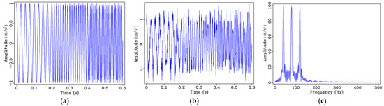
Figure 1. Constant-frequency step signal: (a) Time domain signal; (b) time domain signal with 10% random noise; (c) frequency spectrum of (a).

2.

Linear Frequency-Varying Signal

The second synthetic signal is a linear frequency-varying signal based on the following expression:

$$S_2(t)=\cos [2\pi \cdot (20t+\frac{1}{6}\cdot 500t^2)],\hspace{1em}t\in [0,0.6]$$

(20)

Figure 2 shows the basic characteristics of the (Figure 2a,b) time and (Figure 2c) frequency domains of the signal, which varies linearly in frequency. It can be observed from the frequency spectrum that the difference between constant-frequency step signal and linear frequency-varying signal is that the frequency of the latter changes linearly, and the frequency content ranges between 20 and 120 Hz. As previously stated, it is not possible to see when a certain frequency occurs by looking at Figure 2c.

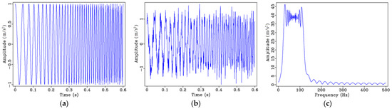
Figure 2. Linear frequency-varying signal: (a) Time domain signal; (b) time domain signal with 10% random noise; (c) frequency spectrum of (a).

3.

Nonlinear Frequency-Varying Signal

The third synthetic signal is a nonlinear frequency-varying signal based on the following expression:

$$S_3(t)=\cos [2\pi \cdot (20t+10t^2+50t^3+60t^4)],\hspace{1em}t\in [0,0.6]$$

(21)

Figure 3 shows the basic characteristics of the nonlinear frequency-varying signal in the (Figure 3a,b) time and (Figure 3c) frequency domains. As can be seen from Figure 3a,b, the change in frequency increases with increasing time, which is due to the nonlinear relationship of time. Figure 3c shows the overall frequency information of the signal, the energy of the low frequency components is stronger, and the signal energy gradually weakens with increasing frequency.

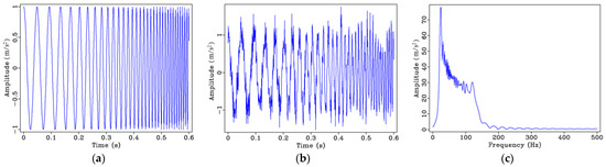
Figure 3. Nonlinear frequency-varying signal model: (a) Time domain signal; (b) time domain signal with 10% random noise; (c) frequency spectrum of (a).

3.2. Time-Frequency Analysis of the Synthetic Signals

1.

Parameter Selection

Among the three time-frequency analysis methods selected in this paper, different parameters can be selected for calculating the STFT and LTFT. For example, for the STFT one can select a time window length depending on the signal analyzed. For the LTFT, a smoothing parameter can be set to control the time-frequency resolution. Taking the constant-frequency step signal as an example, Figure 4 shows the time-frequency spectra calculated by STFT with three different time window lengths. As can be seen, the longer the time window length, the higher the frequency resolution and the lower the time resolution. Thus, when using the STFT, we need to evaluate the time window length according to the characteristics of the signal analyzed, instead of picking a predefined window length.

Figure 4. STFT time-frequency spectra with different time window lengths: (a) 13; (b) 21; and (c) 29 points. The jet colormap is used where blue and red represent low and high frequency magnitudes, respectively.

Figure 5 shows the time-frequency spectra calculated by the LTFT with three different smoothing radii. It can be observed that although there is no significant difference in the time and frequency resolution obtained by the three different smoothing radii, the overlap between the frequency peaks in the time domain increases with increasing smoothing radius. The red boxes in Figure 5 highlight the actual frequency cut-off locations for the example of the 80 Hz peak, which are 0.2 and 0.4 s. Analogous to the STFT, an appropriate smoothing radius should be selected based on the signal analyzed.

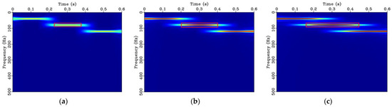
Figure 5. LTFT time-frequency spectra with different smoothing radii: (a) 11; (b) 15; and (c) 19 points. The jet colormap is used where blue and red represent low and high frequency magnitudes, respectively.

2.

Constant-Frequency Step Signal

Next, the three synthetic signals are processed using the STFT (window length = 21 points), ST, and LTFT (smoothing radius = 15 points). Figure 6a,b shows, respectively, the time-frequency spectra of the constant-frequency step signal and its noisy version processed by the STFT. It can be seen that this method can effectively capture all three frequency components. However, owing to the limitation that the frequency resolution is relatively low, if a wider time window is chosen to increase the frequency resolution, the time resolution capability would be lost (see discussion around Figure 4). Figure 6c,d shows the time-frequency spectra of the S transformed signals. The ST offers better time-frequency resolution, especially at low frequencies, while the time-frequency resolution is lower at higher frequencies. It can further be observed that the ST cannot effectively capture the distinct changes in frequency. In addition, like the STFT, the ST spectrum shows notable high-frequency noise for the noisy version of the signal (Figure 6b,d). Figure 6e,f is the result of the LTFT, which has high-resolution regardless of time direction and frequency direction. Not only can it effectively represent the changes at the step edges of the signals, but it is also significantly less sensitive to noise compared to the STFT and ST.

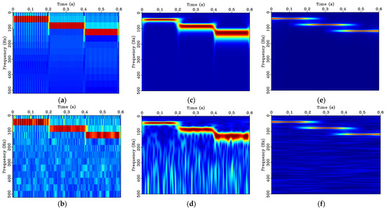
Figure 6. Time-frequency spectra for the constant-frequency step signal: (a) STFT spectrum; (b) STFT spectrum of noisy signal; (c) ST spectrum; (d) ST spectrum of noisy signal; (e) LTFT spectrum; (f) LTFT spectrum of noisy signal. The jet colormap is used where blue and red represent low and high frequency magnitudes, respectively.

3.

Linear Frequency-Varying Signal Model

Through comparison of the three sets of time-frequency analysis for the linear frequency-varying signal illustrated in Figure 7, it can be observed that the STFT spectra do not accurately reflect the linear frequency change of the signal (Figure 7a,b). The ST spectra accurately capture the linear frequency change, but the frequency resolution decreases with increasing frequency (Figure 7c,d). In addition, like the STFT, the ST spectrum shows notable high frequency noise for the noisy signal (Figure 7b,d). Finally, the results of the LTFT are in good agreement with the instantaneous frequency, with high-precision and strong anti-noise characteristics (Figure 7e,f).

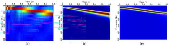
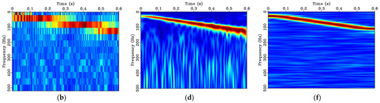
Figure 7. Time-frequency spectra for the linear frequency-varying signal: (a) STFT spectrum; (b) STFT spectrum of noisy signal; (c) ST spectrum; (d) ST spectrum of noisy signal; (e) LTFT spectrum; (f) LTFT spectrum of noisy signal. The jet colormap is used where blue and red represent low and high frequency magnitudes, respectively.

3.

Nonlinear Frequency-Varying Signal Model

For the time-frequency analysis results of the nonlinear frequency-varying signal in Figure 8, the STFT results show discontinuities in signal energy (Figure 8a,b). The problem with the ST results is that the frequency resolution gradually decreases with increasing frequency (Figure 8c,d). As previously noted, both STFT and ST spectra contain a significant level of high-frequency noise (Figure 8b,d). Figure 8e,f highlights again the advantages of the LTFT: high time-frequency resolution across the entire frequency range (Figure 8e,f) combined with a lower sensitivity to noise compared to the SFTF and ST (Figure 8b,d,f).

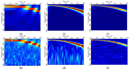
Figure 8. Time-frequency spectrum of the nonlinear frequency-varying signal: (a) STFT spectrum; (b) STFT spectrum for noisy signal; (c) ST spectrum; (d) ST spectrum for noisy signal; (e) LTFT spectrum; (f) LTFT spectrum for noisy signal. The jet colormap is used where blue and red represent low and high frequency magnitudes, respectively.

In order to measure the quality of the time-frequency spectra obtained by the different time-frequency analysis methods and perform an objective evaluation of the time-frequency representation characteristics, we use Rényi entropy, as introduced in Section 2.3. The open-source program implementing Rényi entropy, MIToolbox [33], provided by researchers from the University of Manchester, can be downloaded on GitHub. Table 1 lists the Rényi entropy results for the spectra of each signal. In general, the Rényi entropy value obtained by the LTFT method is the lowest, that is, the time-frequency spectrum aggregation degree, which is a measure of the complexity or information content of the time-frequency distribution, is the highest. As confirmed qualitatively by the spectra plots (Figure 6, Figure 7 and Figure 8), the results obtained by the LTFT have the highest and most consistent resolution compared to the STFT and ST. The time-frequency aggregation degree of the STFT and ST is relatively low. Of the two, the noise sensitivity of the ST is less than that of the STFT.

Table 1. Rényi entropy of the synthetic signals’ time-frequency spectra.

Time-Frequency Analysis Methods	Synthetic Signals
	Signal 1: Constant-Frequency Step Signal Model	Signal 2: Linear Frequency-Varying Signal Model	Signal 3: Nonlinear Frequency-Varying Signal Model
STFT	4.05	7.33	7.38
ST	2.15	2.86	1.47
LTFT	1.13	2.24	1.16

4. Evaluation Based on Experimental Signals

In this section, data collected from a laboratory experiment on a reinforced concrete (RC) girder are analyzed using different time-frequency analysis techniques and then compared.

4.1. Experimental Test Setup

The T-girder used in this study was made of RC and simply supported having a span length of 4.57 m. The concrete’s average cylinder compressive strength was $f_c^{\prime }$= 27.6 MPa and steel reinforcing bars (rebars) had a design yield strength,$f_y^{}$ = 414 MPa. A single load cycle was applied to induce service-level flexural cracking around mid-span of the girder. An elevation view and the cross-section of the girder are provided in Figure 9. More details of this test specimen can be found in [34].

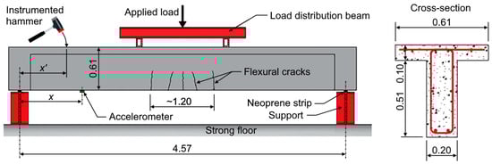
Figure 9. Illustration of experimental test setup. Adapted from [34]. All dimensions in (m).

Vibration tests using an instrumented hammer were performed on the girder before and after cracking had occurred. The hydraulic ram and the load distribution beam shown in Figure 9 were removed for the vibration tests. During dynamic testing, an impact was generated by striking the top of the girder with a 0.68 kg instrumented hammer that is commonly used in impulse response testing. The impact locations range from x^’ = 0.305 to 4.57 m in 0.305 m increments. Each hammer strike was repeated three times to capture measurement variability and determine consistency. The hammer has a built-in piezoelectric sensor to record the time-history of the generated impact force. The signal from the hammer was intensified by a pre-amplifier and digitized using a high-speed data recorder. The girder’s vibration response due to the hammer impact was captured by a capacitive accelerometer (Silicon Designs, Model: 2260-010) attached to the girder soffit. This accelerometer has a relatively flat frequency response (within 3 dB) over a range of 0 to 1 kHz. For this study, three accelerometers were deployed, resulting in five independent positional configurations to cover the fifteen measurement locations. Hence, for each impact location, measurements of the dynamic response from fifteen different locations were available.

The signals from the hammer (=input) and the accelerometer (=output) were digitized and stored by a high-speed data acquisition system (Elsys Instruments, Model: TraNET 204s) using a sampling frequency of 100 kHz. Figure 10 shows the sample of a typical hammer impact signal and vibration response signal from this experiment.

Figure 10. (a) Sample of a typical hammer impact signal and (b) sample of a typical vibration response signal.

During the loading test of the T-girder, a 996 kN capacity hydraulic ram with hand-pump-control was used to apply the load to the steel load distribution beam. The girder was loaded up to 156 kN, which was sufficient to produce service-level flexural cracking around the girder’s mid-span location over a width of approximately 1.20 m.

4.2. Signal Processing and Results

Due to the large amount of test data collected in the original experiment, it is impossible to display all of them in this article. Therefore, for this article we selected the response signals collected by three impact locations and two different positions of accelerometers, i.e., a total of six response signals are studied. In the process of data acquisition, three accelerometers were grouped together. This article takes the data collected by the second accelerometer in each group as an example for extraction and processing. Three impact locations located on top of the girder flange, which is in the compression zone, at x′ = 0.61, 2.44, and 4.27 m. The two accelerometers are located on the soffit of the T-girder, that is, the tension zone, at x = 2.44 and 4.27 m. The locations of the accelerometers correspond to the mid-span and support locations.

• Pre-Damage Signal Processing

In order to facilitate data analysis, it was necessary to number the collected signals of each measuring point. Take the acceleration response signals collected at the eighth collection point and the second impact point before cracking as an example, the collected data is labeled as un8-2. Figure 11 shows the normalized acceleration response signals collected at the three impact locations and the two different accelerometer locations.

Figure 11. Normalized pre-damage acceleration response signals (time domain): (a) un8-2; (b) un8-8; (c) un8-14; (d) un14-2; (e) un14-8; (f) un14-14.

The DFT was performed on the above time-domain signals, and the frequency distributions and amplitude value changes of the response signal in the frequency domain were studied. Figure 12 reveals that the main frequency components with higher amplitude in the acceleration response signals are generally distributed in the range of 0 to 1 kHz.

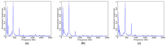
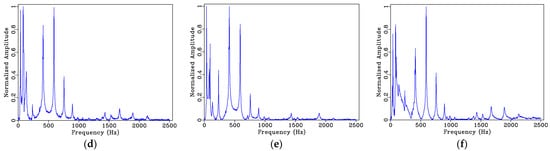
Figure 12. Normalized pre-damage acceleration response signal spectra (frequency domain): (a) un8-2; (b) un8-8; (c) un8-14; (d) un14-2; (e) un14-8; (f) un14-14.

2.

Post-Damage Signal Processing

The acceleration response signals collected at the eighth collection point and the second impact point after damage in the form of cracking, is labeled cr8-2. Figure 13 shows the 6 acceleration response signals received at the 8th and the 14th sampling positions, respectively. It is difficult to see the changes of the T-girder before and after damage in the time-domain signal, so the Fourier transform is applied to observe the change of the signal in the frequency-domain.

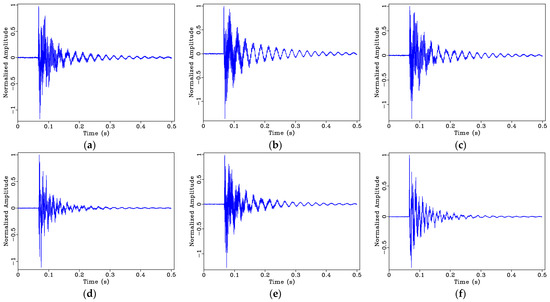
Figure 13. Normalized post-damage acceleration response signal: (a) cr8-2; (b) cr8-8; (c) cr8-14; (d) cr14-2; (e) cr14-8; (f) cr14-14.

Figure 14 shows the stacked spectra at each location, before and after cracking. It can be seen that the frequency response of the signals collected at each sampling point have changed after structural damage in the form of cracking had been imposed. For frequencies greater than 500 Hz, the amplitude attenuation is more obvious, and the position of frequency response of each order has shifted.

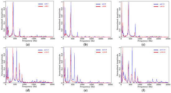
Figure 14. Normalized pre-damage and post-damage acceleration response signal spectra: (a) un8-2 and cr8-2; (b) un8-8 and cr8-8; (c) un8-14 and cr8-14; (d) un14-2 and cr14-2; (e) un14-8 and cr14-8; (f) un14-14 and cr14-14.

The natural frequencies extracted from the spectra are listed in Table 2. Take the data of un14-2 and cr14-2 as an example. It can be observed that the first three natural vibration frequencies exhibit an increase after the T-girder has cracked, which was also observed in [34] and this interesting frequency shifts phenomenon also discussed by Tan [35] and Farrar [36]. For modes higher than three, a significant decrease in the natural vibration frequencies can be observed. This is expected since cracking decreases the stiffness of the girder locally. The reduction varies between 16 and 32 Hz.

Table 2. Natural vibration frequencies of uncracked and cracked girders (un14-2 and cr14-2).

Modes of Nature Frequency	Frequency (Hz)		Shift (Hz)	Shift in %
	Uncracked	Cracked
1	38	42	+4	10.5%
2	84	90	+6	7.1%
3	134	140	+6	4.4%
4	236	220	−16	6.8%
5	412	380	−32	7.8%
6	592	566	−26	4.4%
7	758	730	−28	3.7%
8	896	874	−22	2.5%
9	988	968	−20	2%
10	1068	1048	−20	1.9%

3.

Time-Frequency Analysis

In the above data, the data of un8-8, un14-2 and cr8-8, cr14-2 are selected as representative, the time-frequency transforms were performed using the STFT, ST, and LTFT. The change of the response signals in the time-frequency domain before and after cracking of the T-girder was analyzed. Figure 15 shows the time-frequency transform results of the un8-8 and cr8-8, as the time-frequency spectrum Figure 15a,b shown, the STFT is affected by the window function, the time and time resolution are not optimal. The response signal changes of the T-girder pre and post damage cannot be distinguished visually in the time-frequency domain by the results of the STFT. In contrast, the results obtained from the ST are better than that the ones from the STFT. It can further be observed in Figure 15c,d that the time-frequency spectrum has lower resolution at high frequencies, and the frequency components greater than 750 Hz are not identified accurately enough. Compared with the former two methods, the LTFT can accurately identify each frequency component, and has high time and frequency resolution. In Figure 15e,f, after structural damage, the energy clusters of high-frequency components (758, 1174, 1386 and 1676 Hz) are obviously weakened in the time-frequency spectrum. This can be expected because the propagation path of an elastic wave in concrete changes when the structure is cracked, and the high-frequency components are rapidly attenuated when the elastic wave passes through small pores or cracks.

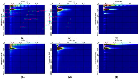
Figure 15. Time-frequency spectra of un8-8 and cr8-8: (a) STFT of un8-8; (b) STFT of cr8-8; (c) ST of un8-8; (d) ST of cr8-8; (e) LTFT of un8-8; (f) LTFT of cr8-8.

Figure 16 shows the time-frequency transform results of the un14-2 and cr14-2, similar to the calculation results of the previous set of data. The LTFT provides superior time-frequency resolution and more details in the time-frequency spectrum compared to the STFT and ST methods. Especially in the time-frequency spectrum calculated after the structure is damaged, it can be seen that the energy clusters in the time direction and the frequency direction are obviously attenuated.

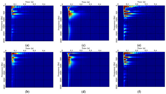
Figure 16. Time-frequency spectrum of un14-2 and cr14-2: (a) STFT of un14-2; (b) STFT of cr14-2; (c) ST of un14-2; (d) ST of cr14-2; (e) LTFT of un14-2; (f) LTFT of cr14-2.

In order to quantify the changes in the time-frequency spectra, Table 3 shows the Rényi entropy of the time-frequency spectrum of the T-girder, pre and post damage, calculated using two sets of data. It can be observed that due to the properties of the signal, the Rényi entropy value from LTFT method is not significantly smaller than the results obtained by the STFT and ST. However, by comparing the Rényi entropy values before and after damage, we can find that the Rényi entropy of STFT does not decrease after structural damage, while the Rényi entropy of ST and LTFT decreases. Meanwhile, due to the attenuation of the high-frequency components, the energy clusters in the time-frequency spectrum are more concentrated in the low frequency region, the time-frequency aggregation degree after the structure has experienced damage is higher than when the structure was intact.

Table 3. Rényi entropy of the experimental signals time-frequency spectrum.

Time-Frequency Analysis Methods	Experimental Signals
	un8-8	cr8-8	un14-2	cr14-2
STFT	1.41	2.28	1.14	1.18
ST	2.33	2.18	1.95	1.62
LTFT	1.79	1.46	1.86	1.57

5. Summary and Conclusions

In this article, a novel time-frequency analysis method based on a non-windowing strategy, namely the local time Fourier transform (LTFT), was presented and evaluated on both synthetic and experimental signals. The LTFT is typically used in seismic data processing, having excellent time-frequency resolution. More traditional time-frequency analysis schemes including the STFT and ST were performed for comparison. Rényi entropy was used as an auxiliary method to effectively compare and quantify the aggregation degree of the time-frequency spectrum. The performances of the three time-frequency analysis methods were first explored using synthetic signals, namely constant-frequency step signal, linear frequency-varying signal, non-linear frequency-varying signal, respectively. Furthermore, a reinforced concrete T-girder was tested, and results are presented and discussed. Finally, the spectral analysis and time-frequency analysis results of the selected vibration response signals are shown to exemplify the effectiveness of the LTFT method for detecting structural damage in the form of cracking.

Overall, we have demonstrated that the LTFT method offers advantages over traditional time-frequency analysis schemes, in that it is more effective for providing high-precision time-frequency resolution and excellent noise suppression. In synthetic signal processing, compared with the STFT and ST methods, the calculation results obtained by the LTFT method always maintain accuracy and high-resolution. Meanwhile, it can be observed that the LTFT method able to suppress some random noise in the whole frequency band. For the laboratory vibration test, the natural vibration frequencies of the selected vibration response signals for modes larger than three were sensitive to cracking as they exhibited a significant reduction. The STFT and ST methods did not show obvious sensitivity to cracking, while the LTFT method could effectively identify the difference between pre and post structural damage from the time direction and frequency direction of the time-frequency spectrum, especially when the frequency is greater than 500 Hz, the energy attenuation of the high-frequency components can be more clearly identified. The calculation results of the Rényi entropy show that the LTFT method has a higher time-frequency aggregation degree than the traditional time-frequency analysis methods. The time-frequency aggregation degree of the post-damaged structure is higher than that of the pre-damaged one. However, the application of time-frequency analysis methods in structural damage detection also has its limitations. At present, this method can only qualitatively identify the existence of damage but cannot quantify the degree of damage and locate the specific location of damage.

Future work includes analyzing impulse response data from a laboratory steel beam. Since compared with the anisotropy in concrete structures, the propagation of elastic waves in steel structures is more ideal. Other tests such as acoustic emission, portable ground penetrating radar, and shaketable testing will be incorporated into future research plans.

References

- Hou, Z.; Noori, M.N.; St Amand, R. Wavelet-based approach for structural damage detection. J. Eng. Mech. 2000, 126, 677. [Google Scholar] [CrossRef]
- Farrar, C.R.; Worden, K. An introduction to structural health monitoring. Philos. Trans. R. Soc. A Math. Phys. Eng. Sci. 2007, 365, 303–315. [Google Scholar] [CrossRef] [PubMed]
- Farrar, C.R.; Park, G.; Allen, D.W.; Todd, M.D. Sensor network paradigms for structural health monitoring. Struct. Control Monit. 2006, 13, 210–225. [Google Scholar] [CrossRef]
- Brownjohn, J.M. Structural health monitoring of civil infrastructure. Philos. Trans. R. Soc. A Math. Phys. Eng. Sci. 2007, 365, 589–622. [Google Scholar] [CrossRef] [PubMed]
- Worden, K.; Farrar, C.R.; Manson, G.; Park, G. The fundamental axioms of structural health monitoring. Proc. R. Soc. A Math. Phys. Eng. Sci. 2007, 463, 1639–1664. [Google Scholar] [CrossRef]
- Tsang, A.H.C. Condition-based maintenance: Tools and decision making. J. Qual. Maint. Eng. 1995, 1, 3–17. [Google Scholar] [CrossRef]
- Amezquita-Sanchez, J.P.; Adeli, H. Signal processing techniques for vibration-based health monitoring of smart structures. Arch. Comput. Methods Eng. 2016, 23, 1–15. [Google Scholar] [CrossRef]
- Maeck, J.; Wahab, M.A.; Peeters, B.; De Roeck, G.; De Visscher, J.; De Wilde, W.P.; Vantomme, J. Damage identification in reinforced concrete structures by dynamic stiffness determination. Eng. Struct. 2000, 22, 1339–1349. [Google Scholar] [CrossRef]
- Brincker, R.; Zhang, L.; Andersen, P. Modal identification of output-only systems using frequency domain decomposition. Smart Mater. Struct. 2001, 10, 441. [Google Scholar] [CrossRef]
- Cheraghi, N.; Zou, G.P.; Taheri, F. Piezoelectric-Based Degradation Assessment of a Pipe Using Fourier and Wavelet Analyses. Comput. -Aided Civ. Infrastruct. Eng. 2005, 20, 369–382. [Google Scholar] [CrossRef]
- Gabor, D. Theory of communication. Part 1: The analysis of information. J. Inst. Electr. Eng.—Part III Radio Commun. Eng. 1946, 93, 429–441. [Google Scholar] [CrossRef]
- Amezquita-Sanchez, J.P.; Osornio-Rios, R.A.; Romero-Troncoso, R.J.; Dominguez-Gonzalez, A. Hardware-software system for simulating and analyzing earthquakes applied to civil structures. Nat. Hazards Earth Syst. Sci. 2012, 12, 61–73. [Google Scholar] [CrossRef]
- Nagata, Y.; Iwasaki, S.; Hariyama, T.; Fujioka, T.; Obara, T.; Wakatake, T.; Abe, M. Binaural localization based on weighted Wiener gain improved by incremental source attenuation. IEEE Trans. Audio Speech Lang. Process. 2009, 17, 52–65. [Google Scholar] [CrossRef]
- Yinfeng, D.; Yingmin, L.; Mingkui, X.; Ming, L. Analysis of earthquake ground motions using an improved Hilbert–Huang transform. Soil Dyn. Earthq. Eng. 2008, 28, 7–19. [Google Scholar] [CrossRef]
- Morlet, J.; Arens, G.; Fourgeau, E.; Glard, D. Wave propagation and sampling theory—Part I: Complex signal and scattering in multilayered media. Geophysics 1982, 47, 203–221. [Google Scholar] [CrossRef]
- Kumar, P.; Foufoula-Georgiou, E. Wavelet analysis for geophysical applications. Rev. Geophys. 1997, 35, 385–412. [Google Scholar] [CrossRef]
- Ghosh-Dastidar, S.; Adeli, H. Neural network-wavelet microsimulation model for delay and queue length estimation at freeway work zones. J. Transp. Eng. 2006, 132, 331–341. [Google Scholar] [CrossRef]
- Rodriguez-Donate, C.; Romero-Troncoso, R.J.; Cabal-Yepez, E.; Garcia-Perez, A.; Osornio-Rios, R.A. Wavelet-based general methodology for multiple fault detection on induction motors at the startup vibration transient. J. Vib. Control 2011, 17, 1299–1309. [Google Scholar] [CrossRef]
- Kim, H.; Adeli, H. Hybrid control of smart structures using a novel wavelet-based algorithm. Comput. -Aided Civ. Infrastruct. Eng. 2005, 20, 7–22. [Google Scholar] [CrossRef]
- Amiri, G.G.; Abdolahi Rad, A.; Aghajari, S.; Khanmohamadi Hazaveh, N. Generation of near-field artificial ground motions compatible with median-predicted spectra using PSO-based neural network and wavelet analysis. Comput. -Aided Civ. Infrastruct. Eng. 2012, 27, 711–730. [Google Scholar] [CrossRef]
- Stockwell, R.G.; Mansinha, L.; Lowe, R.P. Localization of the complex spectrum: The S transform. IEEE Trans. Signal Process. 1996, 44, 998–1001. [Google Scholar] [CrossRef]
- Pakrashi, V.; Ghosh, B. Application of S transform in structural health monitoring. In 7th International Symposium on Nondestructive Testing in Civil Engineering (NDTCE), Nantees, France, 30 June–3 July 2099; NDT: Nantes, France, 2009. [Google Scholar]
- Chen, Y. Nonstationary local time-frequency transform. Geophysics 2021, 86, V245–V254. [Google Scholar] [CrossRef]
- Tary, J.B.; Herrera, R.H.; Han, J.; van der Baan, M. Spectral estimation—What is new? What is next? Rev. Geophys. 2014, 52, 723–749. [Google Scholar] [CrossRef]
- Liu, Y.; Fomel, S. Seismic data analysis using local time-frequency decomposition. Geophys. Prospect. 2013, 61, 516–525. [Google Scholar] [CrossRef]
- Liu, G.; Fomel, S.; Chen, X. Time-frequency analysis of seismic data using local attributes. Geophysics 2011, 76, P23–P34. [Google Scholar] [CrossRef]
- Cohen, L. Time-Frequency Analysis; Prentice Hall: Hoboken, NJ, USA, 1995; Volume 778. [Google Scholar]
- Cohen, L. Time-frequency distributions-a review. Proc. IEEE 1989, 77, 941–981. [Google Scholar] [CrossRef]
- Tikhonov, A.N. On the solution of ill-posed problems and the method of regularization. Dokl. Akad. Nauk 1963, 151, 501–504. [Google Scholar]
- Fomel, S. Shaping regularization in geophysical-estimation problems. Geophysics 2007, 72, R29–R36. [Google Scholar] [CrossRef]
- Fomel, S. Adaptive multiple subtraction using regularized nonstationary regression. Geophysics 2009, 74, V25–V33. [Google Scholar] [CrossRef]
- Baraniuk, R.G.; Flandrin, P.; Michel, O. Measuring time-frequency information and complexity using the Renyi entropies. In Proceedings of 1995 IEEE International Symposium on Information Theory, Whistler, BC, Canada, 17–22 September 1995; p. 426. [Google Scholar]
- Brown, G.; Pocock, A.; Zhao, M.J.; Luján, M. Conditional likelihood maximisation: A unifying framework for information theoretic feature selection. J. Mach. Learn. Res. 2012, 13, 27–66. [Google Scholar]
- Hafiz, A.; Schumacher, T. Effects of elastic supports and flexural cracking on low and high order modal properties of a reinforced concrete girder. Eng. Struct. 2019, 178, 573–585. [Google Scholar] [CrossRef]
- Tan, C.M. Nonlinear Vibrations of Cracked Reinforced Concrete Beams. Ph.D. Thesis, University of Nottingham, Nottingham, UK, 2003. [Google Scholar]
- Farrar, C.R.; Baker, W.E.; Bell, T.M.; Cone, K.M.; Darling, T.W.; Duffey, T.A.; Migliori, A. Dynamic Characterization and Damage Detection in the I-40 Bridge over the Rio Grande (No. LA-12767-MS); Los Alamos National Lab.: Los Alamos, NM, USA, 1994. [Google Scholar]
- Gollob, S. Source Localization of Acoustic Emissions Using Multi-Segment Paths Based on a Heterogeneous Velocity Model in Structural Concrete; Swiss Federal Institute of Technology in Zürich: Zurich, Swiss, 2017. [Google Scholar]
Disclaimer/Publisher’s Note: The statements, opinions and data contained in all publications are solely those of the individual author(s) and contributor(s) and not of MDPI and/or the editor(s). MDPI and/or the editor(s) disclaim responsibility for any injury to people or property resulting from any ideas, methods, instructions or products referred to in the content. |
© 2023 by the authors. Licensee MDPI, Basel, Switzerland. This article is an open access article distributed under the terms and conditions of the Creative Commons Attribution (CC BY) license (https://creativecommons.org/licenses/by/4.0/).