1. Introduction
The application of multi-objective evolutionary algorithms (MOEAs) in design, specifically urban design, has gained momentum over the last decade. The adoption of MOEAs to solve complex design problems has enabled designers to address one of the primary challenges for the design of urban spaces: the ability to simultaneously address multiple design objectives that are in conflict with one another without necessitating trade-off decisions between the design goals. Although the method itself is firmly rooted in computer science and continues to grow as a field [
1,
2,
3,
4,
5,
6], its translation to design and its widespread application is associated with the emergence of various software that do not necessitate coding skills to implement and run the algorithm [
7,
8,
9,
10]. In doing so, access to MOEAs by designers (both for developers as well as users) has been more streamlined than any other point in history, allowing for innovative approaches to responding to, and designing for, design problems comprising multiple conflicting objectives. In urban design, the value of MOEAs is amplified, as it requires a performance-based metric approach to the design problem, allowing designers to integrate climatic, environmental, and urban metrics as key drivers for the algorithm [
11,
12,
13]. This data-driven approach to solving the complexity associated with the urban fabric informs all stages of the algorithmic process; however, key to this is the coupling of the user-driven analysis of the data and the way in which it informs the results outputted by the optimisation run.
Through employing MOEAs in design, three key stages to a successful optimisation run can be identified, each equally significant. The first stage focuses on how the design problem is formulated; this highlights the relationship between three key metrics: the parameters informing the morphology (genes), the morphological characteristics being generated (phenotype), and the fitness functions being optimised for. The way in which these metrics inform each other plays a vital role in a successful optimisation run. The second stage pertains to the algorithm chosen to optimise the design problem; there exists a large number of MOEAs that have been developed over the past few decades, each claiming greater efficiency and success to complex problems [
14]. As such, the chosen algorithm plays a key role in achieving optimised results. The third and final stage is the methods and metrics used to select a solution (or solutions) from the algorithm’s output. Conflicts among the fitness functions driving the MOEA prevent a single optimal solution; rather, what is usually generated, is a number of optimised trade-off solutions [
15]. These trade-off solutions form part of the pareto front (the most optimal solutions generated by the MOEA) and, depending on the size of the generation in the algorithm, the pareto front is composed of a varied number of solutions [
16]—the larger the number, the more challenging it is for the user to select the ‘optimal solution’. The process of selection plays a key role in how the designer rationalises the algorithm’s output—one that is directly correlated with the complexity of the design problem. Design problems with greater diversity in output (driven by greater conflict between fitness functions) demand a rigorous approach to analysis for the purpose of selection—one that is frequently overlooked in the design process.
The research presented in this paper focuses on this third stage of the optimisation process. Through the presentation of a speculative design experiment, evolving an imaginative urban superblock modelled after a high-density urban tissue, this paper presents an adaptable framework for selecting a single solution from the output of an MOEA. The framework employs objective and subjective methods of analysis, both of which are informed by the data generated from the algorithm as well as additional metrics informed by the user. The primary focus of the presented research is the selection mechanisms and processes associated with the application of MOEAs in design, in which the key contribution is a scalable model for designers and users of MOEAs to adapt in their work.
2. Materials and Methods
2.1. Selection Strategy
The advantage of employing an MOEA is primarily due to the algorithm’s ability to solve multiple conflicting objectives without the requirement for the designer to make trade-off decisions; however, in doing so, the algorithm presents a primary challenge to the designer. Optimising for multiple conflicting objectives naturally leads to multiple optimal solutions, where there is no single ‘best’ solution for the designer (in this case referred to as the decision maker (DM)) to select [
1]. There are three points in the optimisation process from where the DM can define a preference for the ‘best’ solution [
17]. The first is before running the algorithm; i.e., during the formulation of the design problem (referred to as priori), in which the DM can skew the algorithm to optimise for one fitness function over the other, primarily through pre-defining weights to the fitness functions. Applying preferences priori transforms the multi-objective problem into a single objective one [
18]. The second point of intervention for preference is during the algorithm itself (referred to as progressive), in which the DM intervenes at different points in the algorithm to direct the optimisation process towards a preferred solution. The third point of intervention is after the algorithmic run (referred to as posteriori), in which the DM chooses a solution from the outputted solution set (this solution is usually selected from within the pareto front). Most MOEAs are classified as posteriori, providing the DM with a set of non-dominated solutions to choose from. The following sections outline a model for designers to choose the ‘best’ solution posteriori.
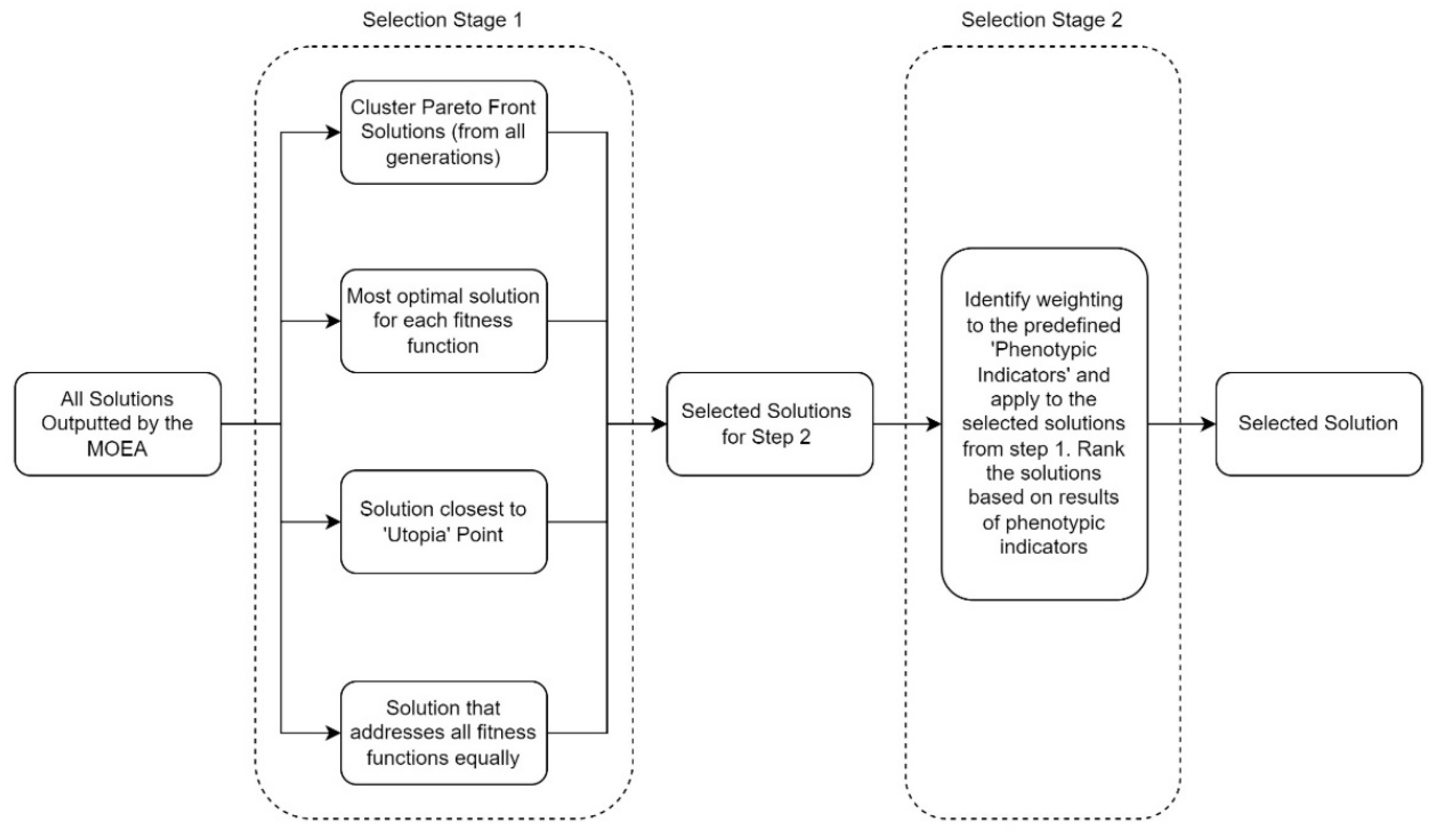
Posteriori selection strategies are primarily driven by quantitative methods of analysis, mainly due to the volume of data generated by the algorithm and the associated population size needed for the algorithm to successfully converge towards optima solutions. Conversely, qualitative selection strategies (if not translated numerically) necessitate a solution set that is small enough for the visual analysis and identification of qualitative conditions not easily represented through quantitative representations. The presented framework combines objective and subjective trade-offs [
19] in a two-stage quantitative and qualitative selection process: the first, a quantitative approach that utilises the fitness functions as the primary metric for selection, and the second, a quantitative and qualitative approach that utilises user-driven ‘phenotype indicators’ for selection. Stage 1 aims to ensure that the entirety of the pareto front is adequately represented while minimising the need to analyse each solution on the front. To do so, various methods are employed to extract solutions from the pareto front, including clustering (for example through k-means or hierarchical clustering methods), fittest solution for each function, solution closest to the ‘Utopia’ point, and the solution with the most equal weight between all functions. From the filtered list of pareto front solutions, Stage 2 requires the DM to analyse the solutions based on additional metrics they find most relevant to the problem being investigated, ranking solutions according to their performance in these user-driven metrics as well as implementing a qualitative selection process through a visual analysis of the filtered solution set (
Figure 1).
2.2. Selection Stage 1
Stage 1 of the posteriori selection process aims to filter the solutions outputted by the algorithm to a manageable size. As designers, there is a vested interest in the phenotypic characteristics of the solutions evolved by the MOEA, thus highlighting a significant advantage to the visual and comparative analysis of the solutions. However, due to the complexity of the problem being investigated and the size of the solution set, conducting this analysis on the entirety of the pareto front may not be feasible. Therefore, the selected subset of solutions from the pareto front must retain the variation and diversity of solutions in the pareto front. To do so, the methods employed in Stage 1 use objective metrics, primarily driven by the fitness values of each solution to facilitate selection. Solutions are selected based on the following four steps.
2.2.1. Clustering the Pareto Front
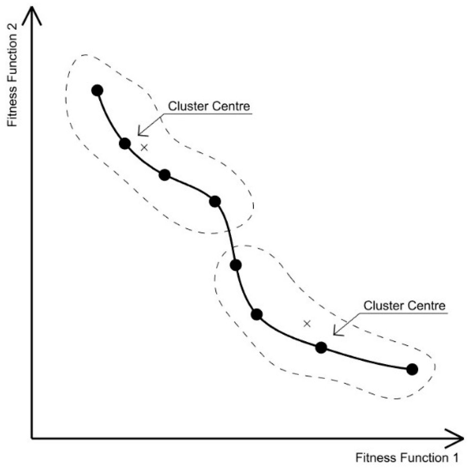
The first step selects a subset of solutions from the pareto front through employing a clustering algorithm (the type of clustering algorithm used should respond to the manner by which solutions are distributed across the pareto front [
20]). The K-value (i.e., the number of clusters) is to be determined by the size of the pareto front, ensuring that each cluster represents a small number of solutions to maintain minimal variation between solutions within a cluster. Doing so ensures that the centre of each cluster (which in this case will be the solution selected) is an accurate representative of all solutions within the cluster. A general guide would be to limit the size of each cluster to between 5 and 15 solutions (
Figure 2).
2.2.2. Fittest Solutions (Outliers)
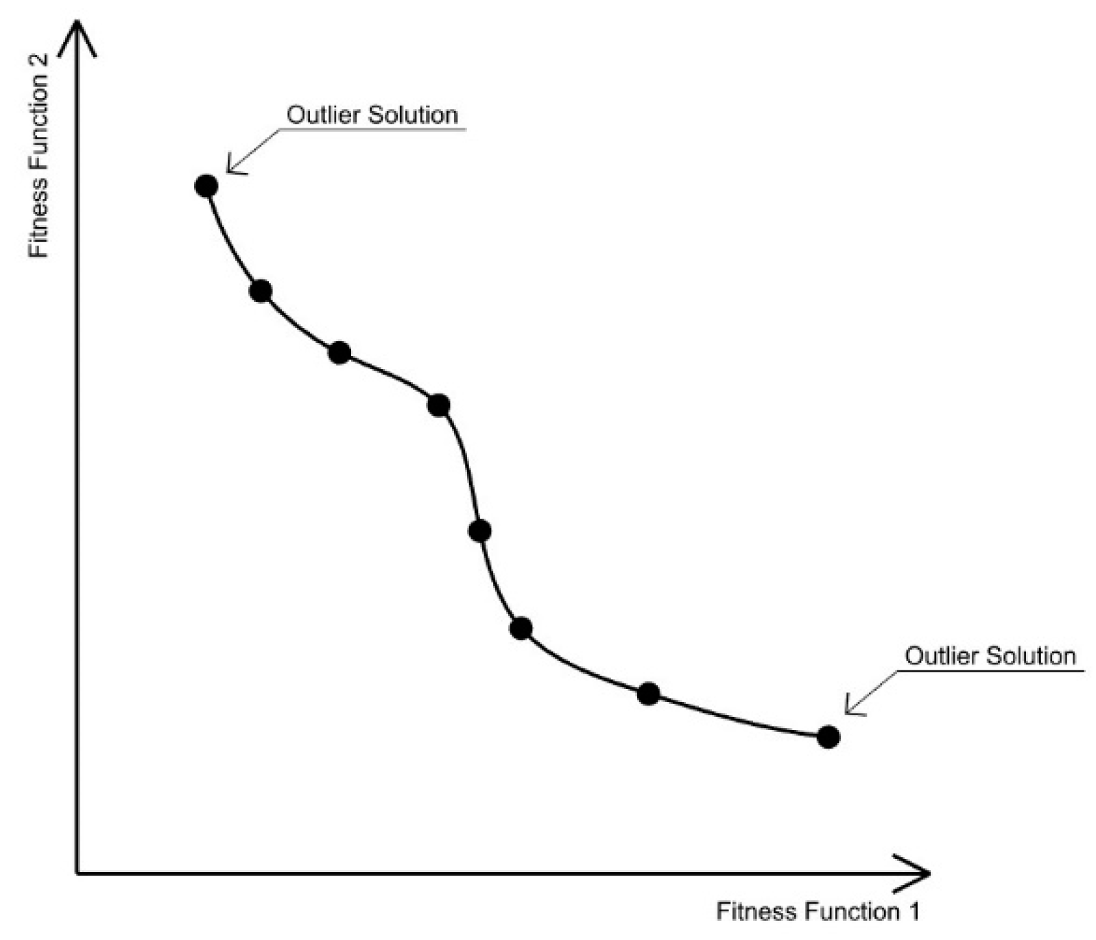
In most cases, clustering the pareto front and choosing the cluster centre for further analysis will minimise the chance for the outlier fittest solutions to be selected. Therefore, the second step selects the fittest solutions for each fitness function for inclusion in the selected pool. As these outlier solutions are less likely to be selected by the DM (since they perform well for one fitness function but poorly for all the others), their inclusion in the selection pool is critical to provide the DM with an indication of the ‘extremes’ generated by the algorithm and the morphological characteristics associated with these extremes (
Figure 3).
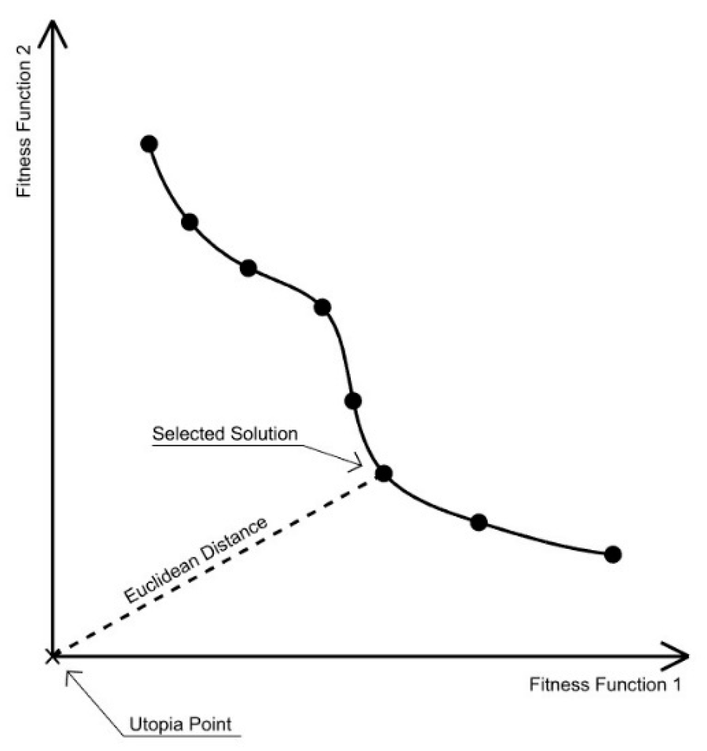
2.2.3. Global Compromise
Yu [
21] and Zeleny [
22] proposed that when the ideal (or ‘Utopia’) solution is not accessible, the next best solution would be the closest one to the ideal solution. In this case, the ideal solution is considered the non-existent optimal solution in the objective space, and thus the selected solution is the one nearest to this point based on a Euclidean measure between the two. This ‘global compromise’ approach is usually considered by decision makers as the solution that best represents all fitness functions and is the closest to the optimal solution; however, this does not automatically translate to it being the ideal solution for the problem being investigated (
Figure 4).
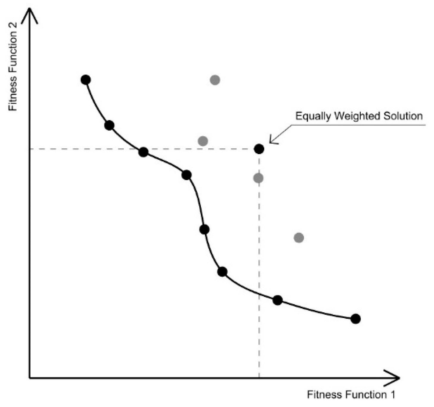
2.2.4. Equal Fitness for All Functions
The final step is to select the solution that holds equal weight for all fitness functions. The ‘Utopia’ solution in the previous step does not correlate to all fitness functions being equally weighted. Where Step 2 selects the outlier solutions, this final step selects the opposite by ensuring each fitness function is optimised equally. It should be noted that this solution may not be located on the pareto front, and may be considered to be a ‘poor-performing’ solution; however, it is the solution that presents the least (if any) trade-offs between fitness functions (
Figure 5).
2.3. Selection Stage 1
Depending on the number of fitness functions of the design problem, along with the number of clusters used in Step 1 above, Stage 1 of the selection process drastically reduces the solution set to one that is more manageable for evaluation (primarily visual) by the DM. Where Stage 1 employed objective metrics for selection, Stage 2 employs a subjective (yet still metric) approach to selection.
The primary challenge with complex urban problems is the number of fitness functions that can be optimised in the MOEA. The greater the number of fitness functions, the more complex the fitness landscape, and thus the ability for the algorithm to optimise the solution set towards a meaningful pareto front [
16]. In most cases, this requires the DM to limit the number of fitness functions used in the algorithm despite there being a comparatively high number of fitness measures that are relevant to the problem. In this context, Stage 2 of the selection process engages with the relevant metrics that were not included in the algorithmic run, utilising them to further analyse the solution pool from Stage 1 and rank the solutions based on how they perform against these added metrics.
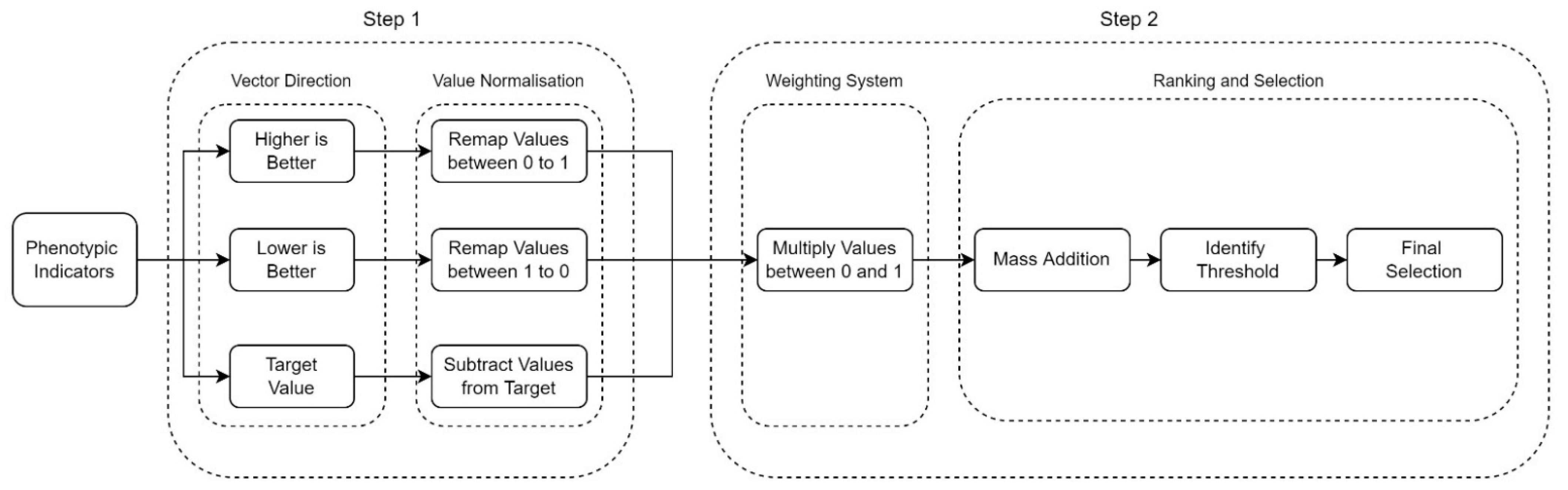
Moreover, as these added metrics are subjective to the DM, their impact on analysis and ranking of the solution pool is equally so. Considering the number of added metrics being analysed for, the DM applies preference through weighting, giving some more priority than others. Despite being a subjective approach, this process remains data driven, requiring the designer to rationalise the analytic and selection metrics through a quantifiable (and reproducible) process (and thus avoid choosing a solution based on visual preference alone). Finally, this approach removes the requirement to limit the number of metrics being used for analysing the filtered solution set, giving greater freedom to the DM as well as providing them with an adaptive model that can be modified to the problem at hand. In this context, Stage 2 of the selection framework comprises two key steps: the first is to identify the metrics for analysis, and the second is to apply weighting to these metrics (
Figure 6).
The following sections demonstrate the application of Stages 1 and 2 of the described selection framework on a speculative high-density urban block. The presented experiment utilises the abstracted morphological and behavioural principles of homeostasis [
23] to inform the evolutionary design processes to evolve an urban superblock with a degree of formal and behavioural adaptation to environmental changes.
3. Case Study
The selection framework presented above is demonstrated through the evolutionary optimization of a speculative urban tissue that examines morphological interventions in the interstitial spaces (the spaces between buildings) of an urban block. The morphological interventions explored in the experiment are driven by Herbert Simon’s argument that the urban fabric’s internal components and external conditions must conform to one another for the city to fulfil its purpose. As such, the case study proposes urban scenarios that connect urban morphologies to dynamic changes and is presented as an extension to radical urbanism through an exploration and habitation of interstitial spaces. The proposed morphological interventions within the urban fabric’s interstitial spaces aim to serve as an explorative study that offer an alternative perspective to urban habitation. The use of an MOEA, and the explorative nature of the evolutionary process, plays a critical role in this explorative study—one that is driven by environmental, micro-climatic, and societal considerations.
3.1. The Design Problem
Rapidly changing environmental and climatic conditions, coupled with the growing numbers of urbanised populations, have stressed the ability of existing cities to cope with these sudden and highly impactful changes. Crossing the critical threshold of stability in a city [
24] is when its population grows beyond its maximum capacity, thus straining its resources and ecological demand, transforming the city into one that is highly sensitive to changes in its environment. Although this is a scenario that has repeated itself multiple times across different geographic locations and periods, its occurrence in modern-day cities carries dire impacts as the current rate of change to environmental conditions is an unprecedented one.
The adaptation of cities that have approached their critical threshold is highly contingent on the rate of change in the environment; historically, the rate of environmental and climatic changes allowed for cities to evolve in response to these changes. However, the rate of environmental fluctuations observed in the 20th century, as well as predicted throughout the 21st century, coupled with the exponential rate of population growth (including the migration of people from rural settlements to urbanised ones) highlights the necessity to re-evaluate the city’s ability to maintain a balanced relationship between the internal processes that govern the city’s growth and development and its environment. Traditionally, the evolution of cities was driven by the adaptation of their spatial distributions in response to a narrow range of change in its environmental context. However, changes in environmental and urban conditions witnessed throughout the last century are occurring at a more frequent and rapid rate, within a broader range and higher intensities.
The vulnerability of urban settlements to environmental disasters (natural or otherwise), has made it necessary to re-evaluate urban morphological configurations. The presented experiment addresses three key elements as part of the superblock’s urban morphology: elevated public networks, the spatial distribution of public space, and the ecological aspects of the city. These three elements are explained briefly in the following section. Future research that focuses on the formulation of the design problem will present the following in greater detail.
3.1.1. Elevating the Flow of the City
The morphology of urban areas and the efficiency by which they grow and occupy their environment has gained significant attention [
25]. Current urban morphologies developed through lateral growth and centralised nodes of activities have two conflicting objectives: first, to be as compact as possible—centralisation; and second, to be as dispersed as possible—decentralisation [
26]. In recent years, the dramatic increase in urbanites has placed tremendous demand on the spatial distribution and resource management of existing urban settings. Although its impact naturally leads to verticality, this has been implemented within the scale of a single building, yet the city’s flow continues to grow laterally at ground level. As a result, the programmes that are dependent on this circulatory system are being distributed at the street level, while buildings continue to develop as separate entities vertically. This led to Harvey Wiley Corbett, primarily known for his skyscraper designs, to be one of the first figures to suggest in the early 20th century the integration between multi-level street networks and mixed-use skyscrapers [
27]. Patterns of settlements in many urban areas are transforming from dispersed fabrics to centralised entities with integrated infrastructures [
28], mostly in the form of segregated and standalone mixed-use buildings. However, there are cities where the application of higher-level connections has been proven to benefit the urban context. In Hong Kong, traffic congestion, accompanied by air and noise pollution, are the reasons for the incorporation of high-level connections within an urban block. While in Minneapolis and Calgary, their application was in response to the region’s severe climatic conditions, leading to an 18-km network of higher-level connections throughout the urban fabric. In addition to the climatic advantages, Corbett et al. [
29] argue that such spatial relationships allow for greater and more efficient circulation paths across the urban morphology.
Elevating the flow of the city is one of the urban objectives considered for the presented case study. The spatial proliferation of different urban activities across the urban morphology leads to the emergence of interstitial spaces at different heights with different spatial attributes.
3.1.2. Spatial Distribution of Public Space
The physical and social structures of a city have a reciprocal influence on one another as they continue to develop [
26]. Interactions between individuals occur at different spatial scales and locations within a city. However, these networks of interactions are not constrained to their physical structures and surpass the current physical attributes of cities. Public spaces across the city are examples of such areas, where the spatial structure facilitates the social interactions of its inhabitants. The majority of public spaces accessible to the public are located at the street level, while the network of interactions goes beyond a singular level. According to Frans Dieleman and Michael Wegner [
30], one of the consequences of urban sprawl is the loss of open space; therefore, by allowing the vertical development and distribution of public space, the morphology and its organisational structure would transform the conventional spatial distribution of an urban sprawl. Although an urban patch may be constrained to its geographical boundaries at the ground level, thus limiting the development of public spaces, the vertical distribution of such spaces bypasses this constraint. Such spaces have great potential to be considered not as confined areas but as a network of spaces connected through higher-level connections.
The distribution of public spaces on multiple levels is another urban objective that is addressed through the presented case study. However, rather than emerging as a by-product of the spatial distribution of buildings, the experiment designates a distinct identity to the interstitial spaces across different levels, allowing for their propagation throughout the urban morphology.
3.1.3. Ecology and Spatial Qualities of the City
Changing environmental and climatic conditions, coupled with a growing demographic, has challenged cities’ ecological capabilities to adapt to these fluctuations. The strains of energy consumption have substantially influenced cities’ internal environmental and ecological contexts. Processes of urban development, more particularly, urban morphological configurations and reconfigurations, influence the city ecology across a range of spatial domains—from interstitial spaces to the regional environment. As such, ecological systems are dynamic and continuously adapt to other components, such as social and biophysical ones [
31]. Therefore, an urban ecological model is integral to the adaptability and flexibility of an urban area. In contrast to many of the planned cities of the 20th century, evolving cities have been closely coupled to their immediate territories, with distinct morphologies, integrated infrastructure, and urban cultures that have evolved in response to the specific ecological and climatic conditions of the region. As these cities grow and develop in complexity, they have become less dependent on their immediate surroundings by obtaining the required energy demands from their local territories [
23]. The exchange of energy between the built structures of the urban fabric and the surrounding environment is influenced by the spatial distribution of the urban morphology. It also influences the microecology of interstitial spaces across a range of temporal and spatial scales in the tissue. Therefore, morphological relationships across the urban fabric, such as volume-to-surface ratios [
32], surface resolutions, proximities of the buildings, and the spatial relationships between the different components, play a crucial role in adaptation to different environmental conditions and the ecology of a city at large.
Enhancing ecological interactions, more particularly, the energy exchange expressed via intricate spatial distribution of spaces across the urban area, is another urban objective in the presented case study, examining the energy exchange between the built environment of the urban fabric and the interstitial spaces evolved as a result of the spatial distribution of buildings.
3.2. Experiment Setup
3.2.1. Spatial Distribution of Public Space
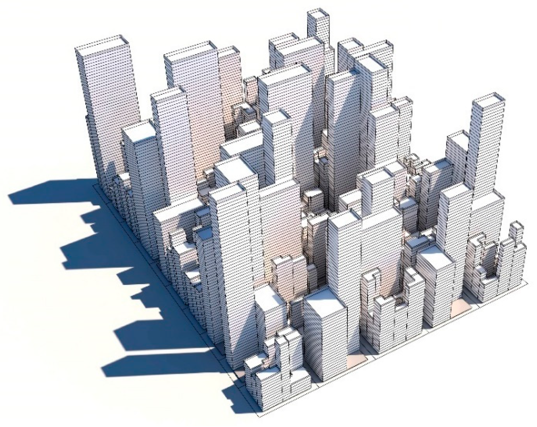
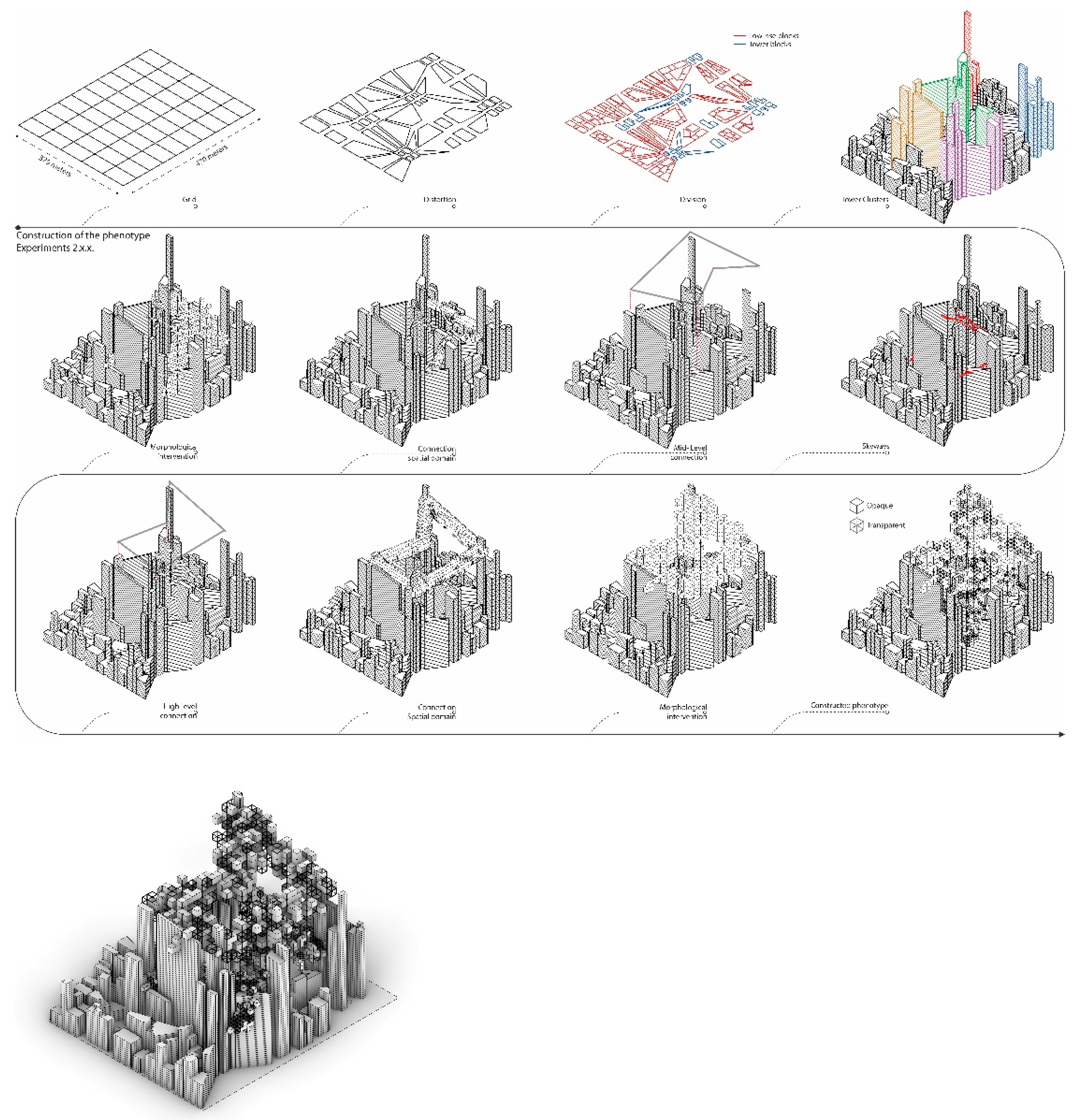
The base phenotype for the presented experiment imagines a high-density urban block (
Figure 7) as the basic geometric component. The phenotype comprises a 5 × 10 grid layout that spans over 375 m in width and 470 m in length. The orthogonal grid structure is distorted in several locations to enable the phenotype to break free from the grid should the algorithm favour such a change. By allowing the nonorthogonal formation of the grid, it enables the building footprints to cluster in different proximities, leading to an increase in variation of the interstitial spaces throughout the urban tissue. The generated footprints were divided into two distinct categories, namely, low-rise building blocks and tower blocks, according to their areas. The morphology comprises rectangular footprints that are distributed amongst the building blocks, with heights varying from 5 to 25 stories.
The low-rise building blocks develop alleys and central courtyards. The tower building blocks comprise two high-rise buildings and an open corner at the street level to serve as the open plaza for each tower. A network of open spaces, comprising the courtyards and open plazas, is formed, which is distributed across an extended network of streets and alleys with different widths and lengths at the ground level. A set of transformations control the attributes of this network and consists of the building heights and footprints as well as the size of the street networks and alleyways.
Tower blocks across the urban tissue cluster into five groups based on their proximities. The shorter tower of each group is designated as the connection point of the skyways that locally connect the towers of the cluster. As the rate of the towers grows in the phenotype, the frequency of the skyways increases and enables circulatory paths to emerge between the towers in close proximity.
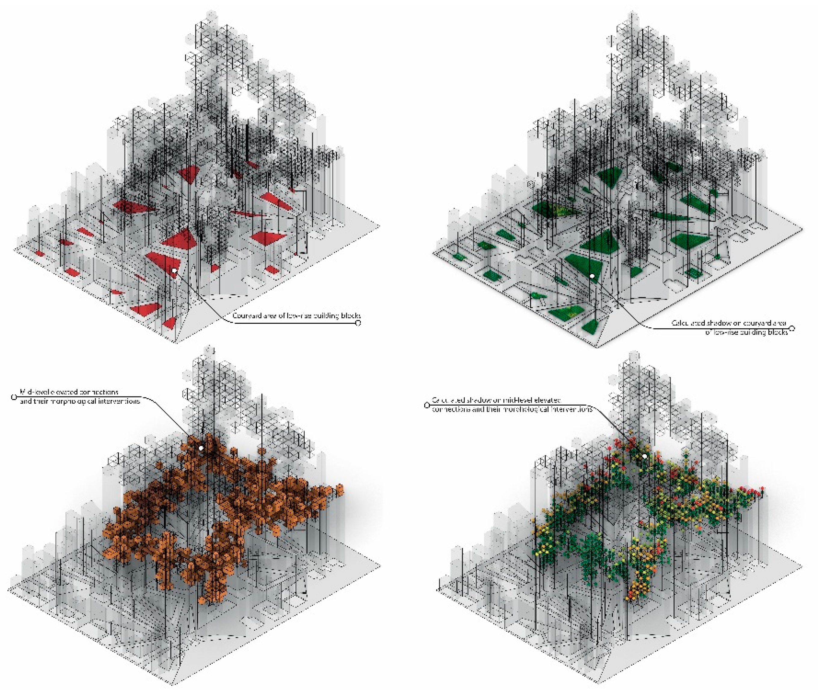
The phenotype is constructed to enable elevated connections to emerge across the urban fabric for two primary reasons: first, to extend the circulation beyond the street level, and second, to provide a blueprint for further development of the city should the population expand to its maximum capacity. In addition to the skyways in each tower cluster, a set of higher-level connections that stretches over the entire urban fabric are designated in the phenotype. To ensure that additional higher-level connections across the elevation cover the entirety of the urban area, but which will not overshadow the ground level excessively, the phenotype comprises a set of genes that allows higher-level connections to emerge across the urban fabric at two different elevations. The higher-level connections across the urban area are achieved by enabling spatial units to emerge across the tissue should simulation favour such a change. These spatial units facilitate the morphological intervention of the urban form.
The mid-level elevated circulatory networks connect the towers in the urban tissue while developing a point of contact with the low-rise building blocks. The high-level elevated connections grow from the tallest towers within each cluster and circulate around the urban fabric and create a ring of horizontal habitable spaces. The transformations within the genome of the phenotype control the length, distance, and surface area of these elevated connections, to ensure adequate solar gain on the ground level, adequate solar gain on the elevated surfaces, and their accessibility across the urban fabric. Through interactions between the buildings (low-rise and towers) and the elevated connections, various interstitial spaces with unique spatial qualities emerge across the tissue. The benefit of the morphological interventions (through adding spatial units, voxels) of the elevated connections for the urban area is threefold: first, to elevate the flow of the city; second, to enable habitable spaces to emerge in the interstitial spaces between towers; and third, to develop a balance between horizontality and verticality, to attain a higher density. The chromosomes that define the phenotype’s construction are presented in
Figure 8.
3.2.2. Fitness Functions
A multitude of metrics have been identified to optimise the developed phenotype. Four of these metrics have been selected as the fitness functions within the MOEA (
Figure 9), while the remainder will be utilised for the purposes of analysis and selection (presented in Stage 2 of the selection framework).
The first fitness function concerns the solar gain on two categories of spaces across the urban tissue: the first is the generated courtyard areas in the low-rise building blocks, and the second is the outer surfaces of the mid-level elevated connections. By controlling the solar gain on the courtyard areas, the algorithm attempts to explore various distributions of low-rise and tower blocks across the urban tissue. This naturally leads to the emergence of unique interstitial spaces across the ground level. Simultaneously, the second part of this objective (to control the solar gain on the mid-level elevated connections) forces the simulation to explore the spatial distributions of mid-level elevated surfaces in relation to the urban morphology. It creates elevated surfaces across different levels of the urban area that can be utilised for outdoor urban activities (
Figure 10).
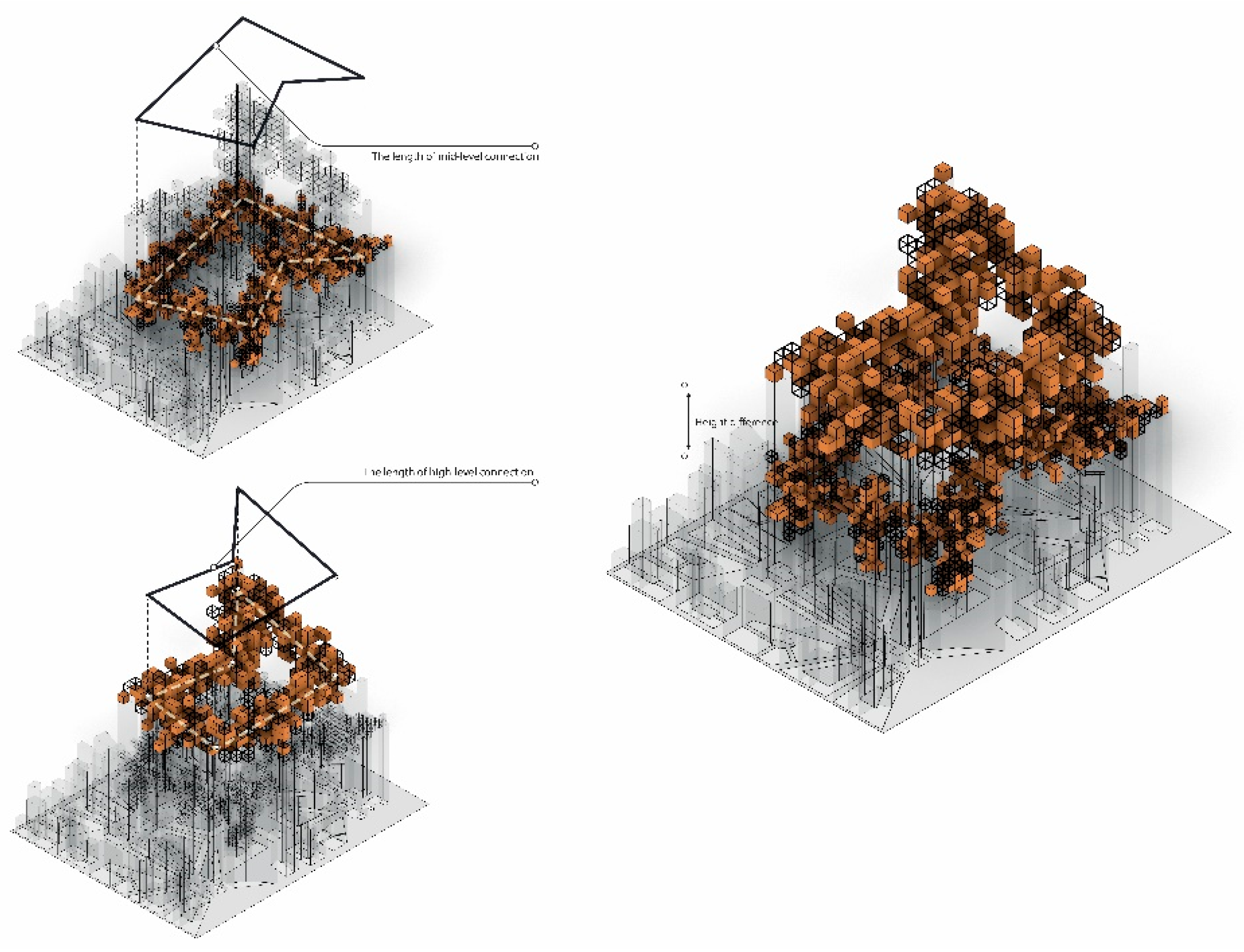
The second fitness function increases the length of the mid-level and high-level elevated connections and the distance between them. As previously discussed, the phenotype is created to facilitate the development of elevated connections across the urban fabric for two primary reasons: to extend the circulation beyond the street level and to provide a blueprint for further development. Thus, the fitness function is defined to increase the length of these elevated connections (both mid-level and high-level) as well as to encourage their distribution in elevation. By doing so, solutions with elevated connections that are stretched horizontally and vertically across the urban tissue are favoured. As a result of this spatial distribution, interstitial spaces with unique spatial qualities emerge at different levels across the tissue (
Figure 11).
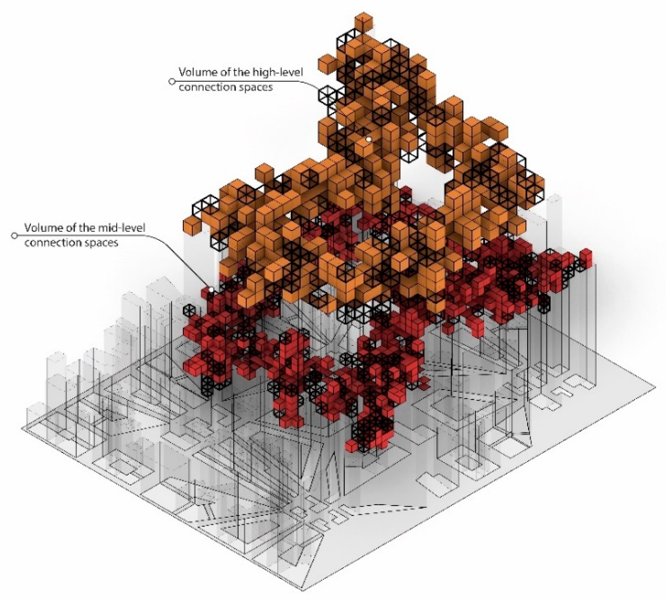
The third fitness function increases the volume of the elevated connections and the surface-to-volume ratio. This fitness function focuses on the formation of elevated connections throughout the urban tissue. It is defined to increase their volume as well as the ratio of their surface area to their volume. By increasing the volume of the elevated connections, the simulation generates solutions with volumetric connections that can be considered as extensions to the current urban morphology and be utilised as habitable spaces. It provides an alternative urban morphology for increasing density horizontally and vertically. The increase in the ratio of the surface area to volume contributes to self-shading mechanisms and produces shaded elevated outdoor surfaces (
Figure 12).
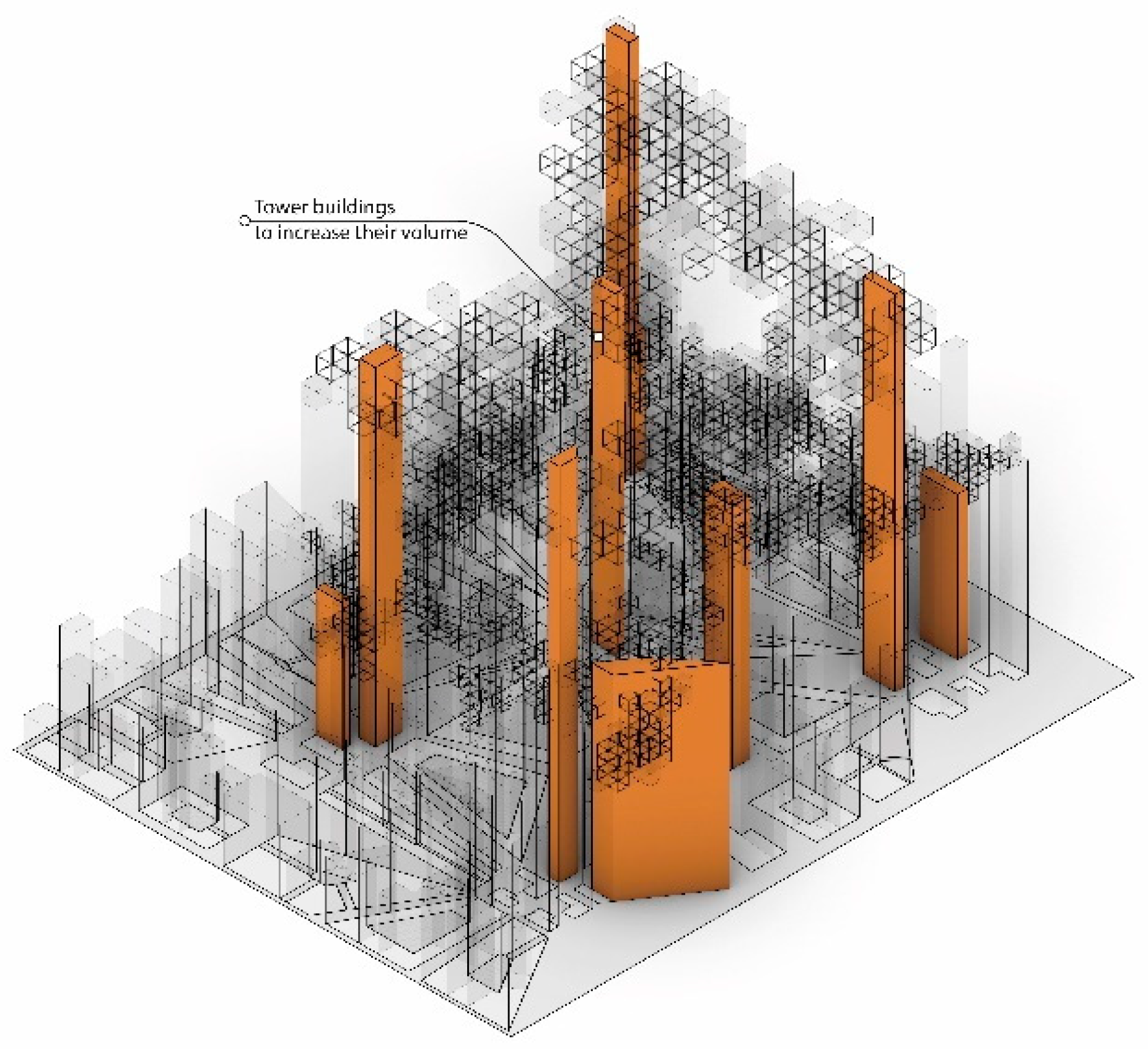
Finally, the fourth fitness function increases the built volume of the towers. This fitness function drives the algorithm to evolve larger tower blocks which are associated with an increase in density. Due to the elevated connections being attached to the tower blocks, increasing the volume enhances the structural performance of the buildings to which the elevated connections are connected (
Figure 13).
3.2.3. Algorithm Settings
The design problem presented above was run in the software Wallacei [
9], which utilises the NSGA-2 MOEA developed by Deb et al. [
33]. The algorithm was run on a consumer-grade laptop with the following settings (
Table 1) and specifications: Intel Core i7, 2.4 GHz processor, and 32 GB Ram.
4. Results
4.1. Algorithm Results
Although the presented research focuses on the selection mechanisms employed on the algorithm’s output, an overview of the algorithm’s results is presented. As can be observed from
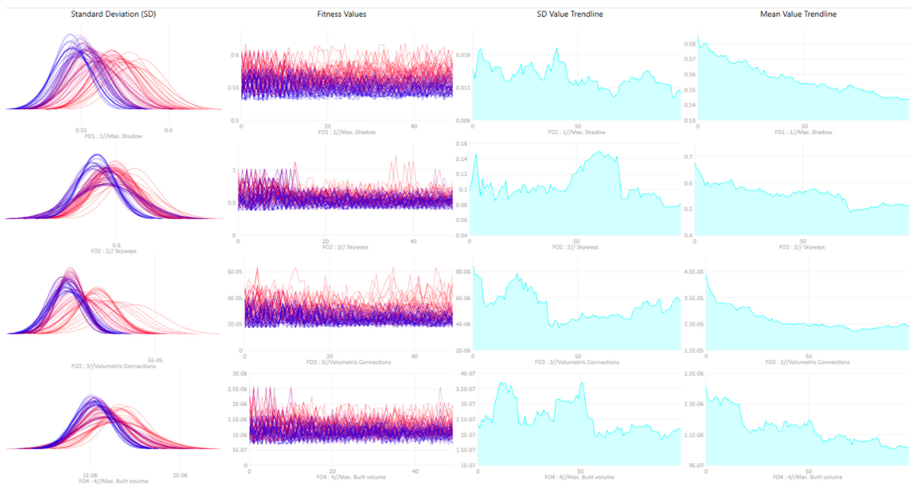
Figure 14, all four fitness functions exhibit varying degrees of convergence towards local optima, with Fitness Functions 1 and 3 (shadows and volumetric connections) displaying a more evident improvement in fitness throughout the evolved generations. In contrast, the other two objectives (skyways and built volume) are comparatively less so: although presenting improved fitness overall, they are slower in converging towards an optimum. As discussed in previous sections, the formulation of the design problem is key, and although outside the scope of this paper, the successful optimisation observed in the algorithm’s output is a result of multiple iterations of reformulating the design problem, constantly striving to find a balanced relationship between the chromosomes, phenotype, and fitness functions.
4.2. Selection
As discussed in the Materials and Methods section, the proposed selection framework comprises 2 stages: an objective Stage 1, which filters the population down to a manageable solution pool, and a subjective Stage 2, which ranks the solution pool based on weighted indicators. The results from these two stages are presented below.
4.2.1. Selection Stage 1
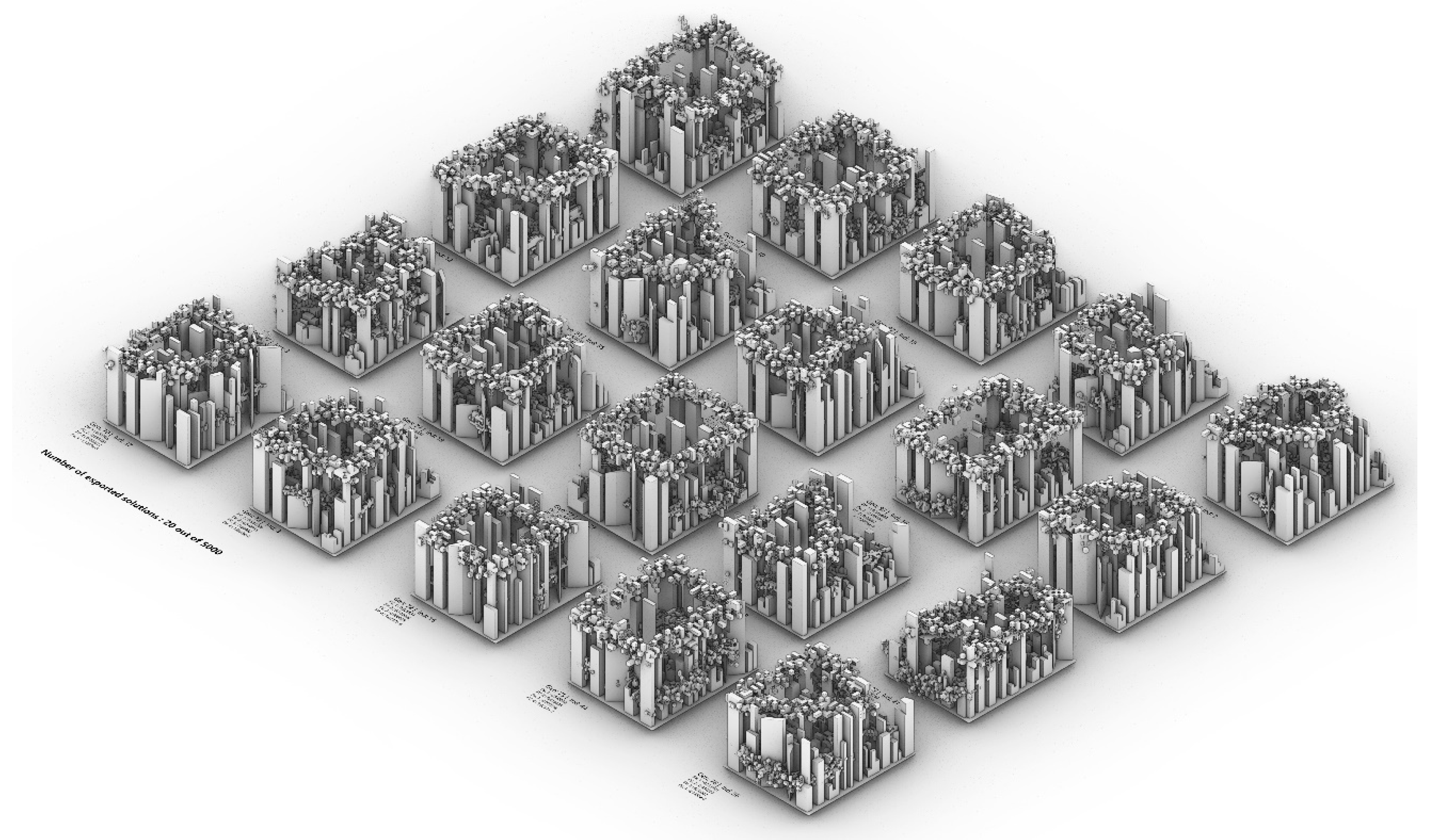
Stage 1 filters down the population using four steps. Step 1 applies a clustering algorithm on the pareto front of the entire population. In the case of the presented experiment, the MOEA resulted in 120 pareto front solutions. A hierarchical (average linkage) clustering algorithm was employed, with a K-value of 20 and an average cluster size comprising 8 solutions (
Figure 15). The solution closest to the centre of each cluster was selected and added to the solution pool (
Figure 16).
Step 2 selects the ‘outliers’ in the pareto front; i.e., the fittest solution for each fitness function (
Figure 17). As the fitness functions in the design problem are conflicting, the fittest solution for one function usually exhibits poor fitness for other functions.
Step 3 selects the solution closest to the ‘Utopia’ point (
Figure 18). Identifying this solution requires a simple Euclidean calculation between the ‘Utopia’ point (x), which in this case has a vectorial value of 0,0,0,0, and the normalised vectors of all the solutions in the pareto front (y). The solution with the shortest Euclidean distance is closest to the ‘Utopia’ point. An example of this calculation is provided below:
Finally, Step 4 selects the solution that exhibits an equal weighting (or the closest equal weighting) between all four fitness functions (
Figure 19). Identifying this solution requires the normalisation of the fitness values for all fitness functions and selecting the solution with the same normalised fitness value for all functions. Plotting this solution on the parallel coordinate plot and on the diamond chart should present a straight line and an equilateral diamond, respectively. If there exists no solution with an exactly equal weighting between the fitness functions, such as the example presented here, the closest solution to the ‘ideal’ equally weighted solution is selected. As described previously, and unlike the three steps outlined above, this solution may not fall on the pareto front (which is the case in the selected solution).
Through the selection mechanism of Stage 1, the solutions selected from the population have been filtered down to a solution pool comprising 26 solutions. Most importantly, however, these 26 solutions represent and maintain the diversity generated in the pareto front while simultaneously allowing for a visual analysis of the results.
4.2.2. Selection Stage 2
In contrast to the objective selection mechanisms presented in Stage 1, the second stage of the selection framework requires a high degree of subjective decisions by the DM, who in this case is the person with the greatest expertise on the problem being investigated. However, selection based on purely visual analysis negates the data-driven approach that has so far been utilised in the MOEA process. Therefore, Stage 2 requires the DM to identify relevant ‘phenotypic indicators’ that evaluate each solution in the filtered solution pool. These indicators provide two key advantages to the DM: first, they provide a metric approach to analyse the solutions and identify differences between them that go beyond the metrics used in the fitness functions (optimised by the algorithm); and second, through using a numeric approach to evaluate the solutions, weighting can be applied to the metrics used, giving the DM the ability to dictate priority of metrics for selection, driven by the parameters that define the design problem. In both steps above, the DM can respond to external demands imposed on the project by additional stakeholders that are not directly involved in the problem’s formulation.
The metrics identified to be relevant to the problem being investigated are listed in
Table 2. Note that it is critical for the DM to normalise all the metrics as well as identify the direction of each metric (i.e., is it better to minimise the value, maximise the value, or drive it towards a specific target value). Once the metrics have been calculated for each solution in the solution pool, Step 2 applies various weights to the calculated metrics; this step is critical, as it provides added agency to the DM to select solutions based on rationalised and quantified subjective decisions. The final step is to add the resulting values for all metrics per solution; this provides the DM with a single number that represents the rank of each solution based on the results of the ‘phenotypic indicators’.
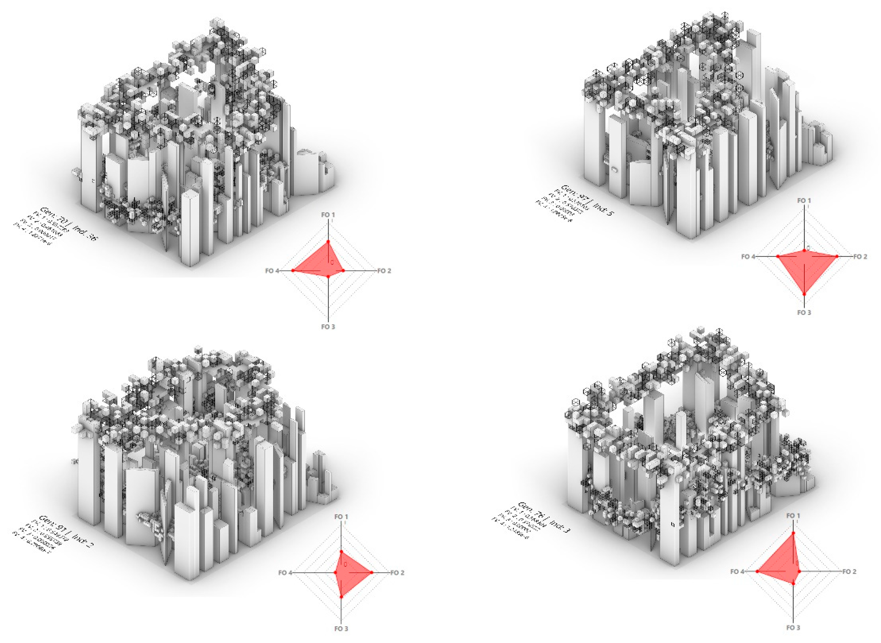
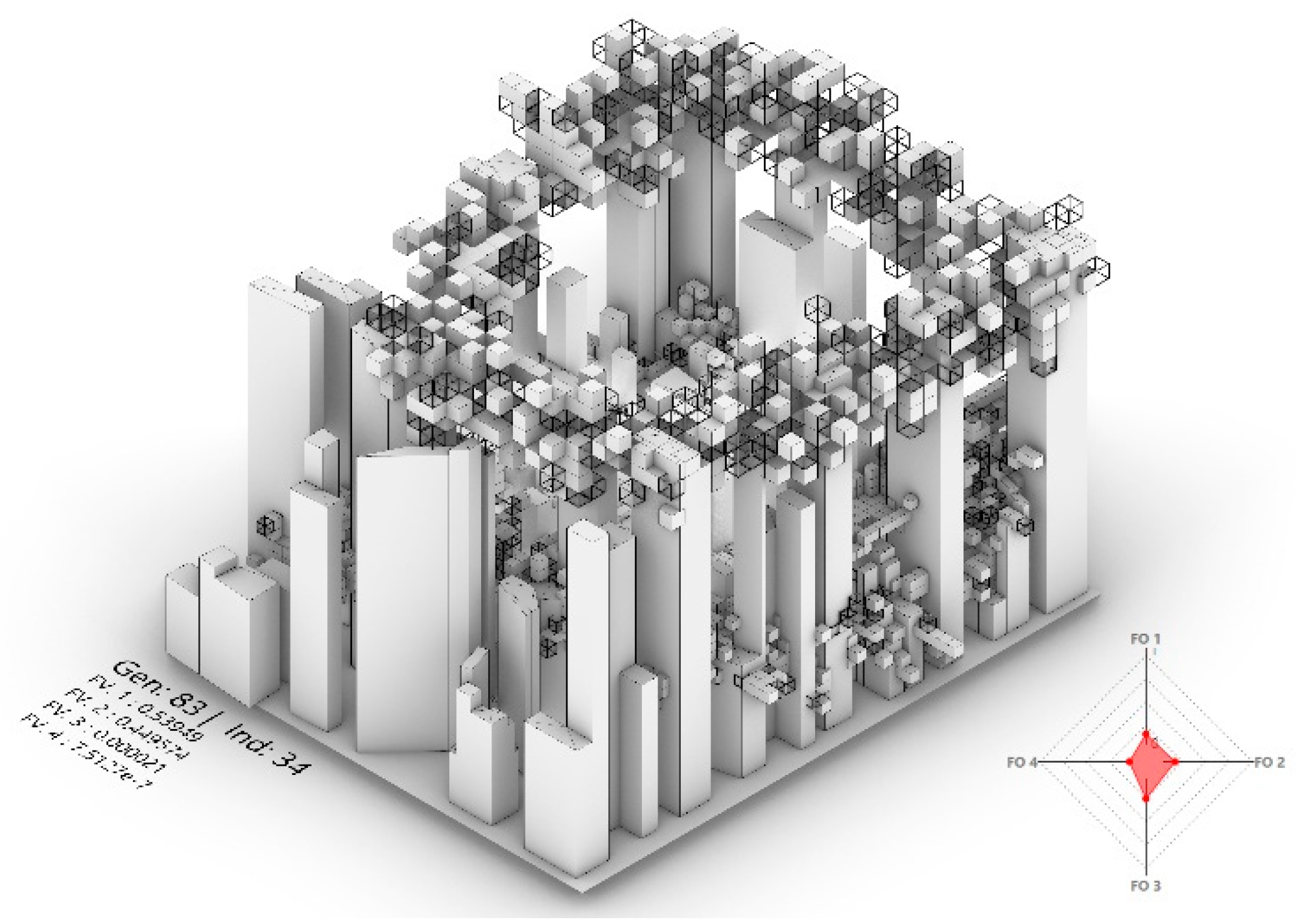
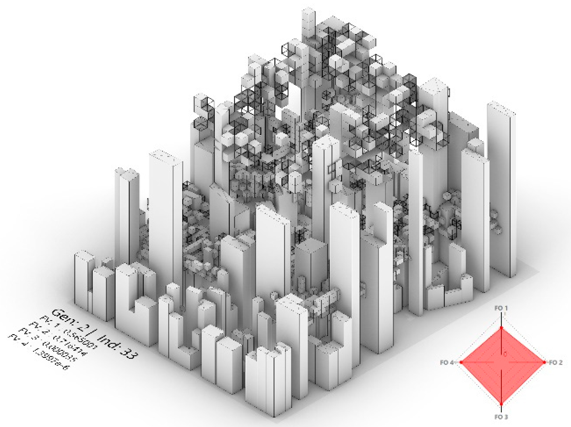
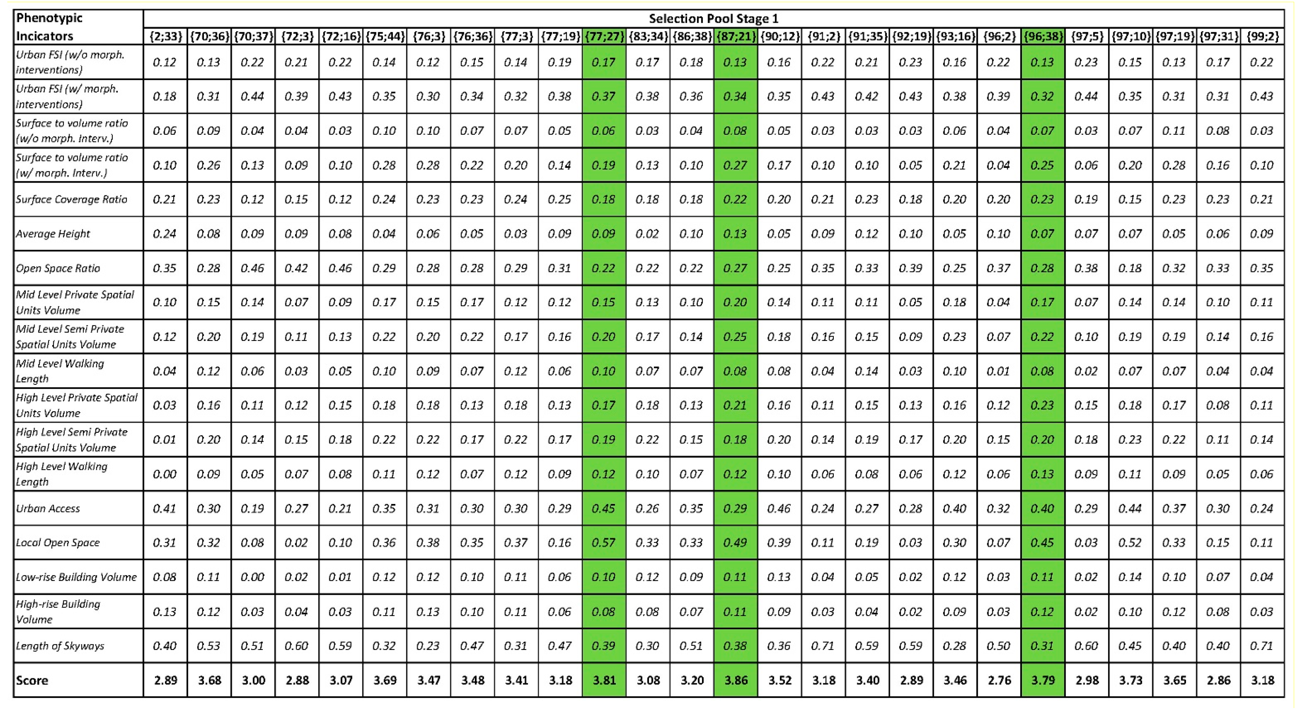
The phenotypic indicators, along with the defined weighting for each indicator, were applied to the solution pool from Stage 1. The results and ranking are presented in
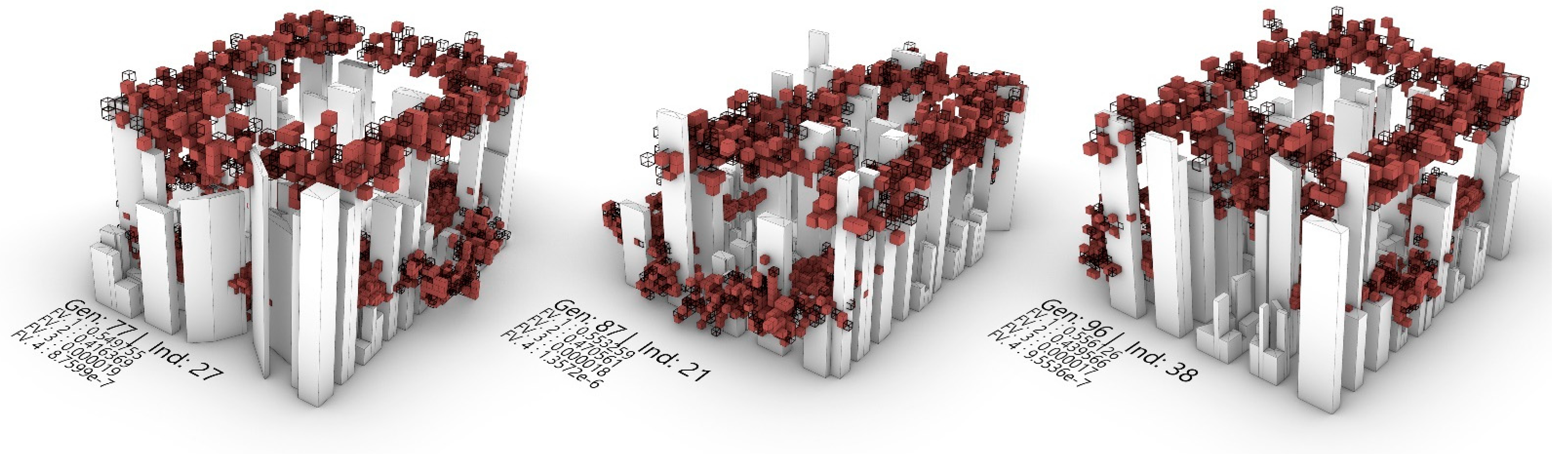
Figure 20. The three top solutions, with a ranking above a certain threshold (in this case 3.80), were selected for selection by the DM (
Figure 21).
5. Discussion and Conclusions
The application of MOEAs in design, specifically urban design, requires the decision maker to critically review all aspects associated with the algorithmic process. Although the formulation of the design problem, and the chosen algorithm to run the simulation, are critical for generating successful results, the method for selecting the ‘best solution’ from a population of solutions that are all non-dominated (i.e., improving one solution will make another one worse) is considerably consequential. The selection method presented in this paper proposes a framework for designers to evaluate and filter a larger solution set through both an objective and subjective process, each equally significant.
To demonstrate the proposed selection framework, a design problem comprised of a speculative urban tissue was developed to respond to contemporary urban and environmental objectives; that is, to evolve urban configurations comprised of intricate spatial and morphological organisations within the urban fabric’s interstitial spaces. The conflicting nature of the fitness functions driving the experiment resulted in wide-ranging diversity amongst the optimised solutions, demanding a critical and thorough selection process that filters through this variation by both quantitative and qualitative modes of analysis.
The key objective of the proposed selection framework is to maintain diversity in the filtered solution set while delivering a pool of solutions that is feasible for visual analysis. In Stage 1 of the selection framework, four key selection mechanisms are applied. Clustering the pareto front (with a high K-value) ensures that all solutions are represented in the filtered solution pool, while selecting the fittest solutions for each objective ensures the DM incorporates the outliers of each fitness function in the solution pool. Moreover, the outlier solutions provide the DM with the domain of the pareto front. Selecting the solution closest to ‘Utopia’ provides the DM with the result that is in the nearest proximity to the ideal (non-existent) solution to the problem, while the final mechanism for selecting the solution with the most equal weight delivers the result that applies no trade-offs to the fitness functions. These four selection mechanisms provide the DM with an objective and comprehensive representation of the optimised results.
Although Stage 2 aims to apply subjective decisions for analysis and selection, filtering the solution set to a manageable size in Stage 1 equips the DM with the ability to visually inspect the results of Stage 2. As discussed, the subjective approach in Stage 2 requires the DM to identify additional metrics (phenotypic indicators) to further analyse the results. Although not essential, there is added value to weighting the phenotypic indicators according to their importance to the problem being investigated. This added value increases as the number of phenotypic indicators. Once the solutions are evaluated and ranked, the DM may choose to visually inspect the top solutions and apply an additional layer of analysis to those top solutions, or choose the best solution based on the ranked results. The results in the case study presented herein intentionally avoided selecting the best solution, instead proposing the top solutions for the DM to choose from. The DM’s role in visually inspecting solutions and making subjective decisions remains critical to the design problem; however, this process is significantly strengthened when complemented with a numerically rationalised objective and subjective evaluation process.
Although the primary mechanism for maintaining diversity in Stage 1 is through clustering the pareto front, the clustering algorithm is applied on the fitness values of the solutions. Despite the algorithm successfully grouping solutions based on the Euclidean proximity of their fitness values, this does not necessarily translate to phenotypic similarity. It is possible for two solutions to present fitness similarity while simultaneously maintaining phenotype diversity [
34]; therefore, future work should focus on integrating (or replacing) fitness clustering with genomic clustering for an accurate correlation between the clusters and morphological characteristics of the selected solutions. It is critical to highlight that the presented framework is highly adaptable to the problem at hand. Although the four steps of selection in Stage 1 aim to maintain diversity, the DM may employ additional selection mechanisms to add solutions to the filtered solution set. Such selection mechanisms include the Knee-Point solution, located on a ‘bulge’ or ‘knee’ of the pareto front [
35], or the average ranked solution (the solution with a mean ranking between fitness functions) [
36]. In Stage 2, the phenotypic indicators most relevant to the DM should be applied for evaluation; these indicators will widely differ based on the problem being investigated, for example metrics that specifically address liveability and quality of life (such as walkability, privacy, access to daylight and ventilation, etc.). Fundamental to this process is the user’s ability to numerically quantify the urban condition being analysed. Although the presented indicators do not consider opportunities for temporal growth or adaptive response of the generated solutions, integrating metrics related to these modes of analyses for the purposes of selection is made possible through favouring variation over optimisation; however, a priori approach to adaptive growth remains the most suitable approach.
Author Contributions
Methodology, M.S., M.M.; Case Study, M.S.; analysis, M.S., M.M.; writing—original draft preparation, M.S., M.M.; writing—review and editing, M.S., M.M. All authors have read and agreed to the published version of the manuscript.
Funding
This research received no external funding.
Institutional Review Board Statement
Not applicable.
Informed Consent Statement
Not applicable.
Data Availability Statement
Not applicable.
Conflicts of Interest
The authors declare no conflict of interest.
References
- Deb, K. Multi-Objective Optimization Using Evolutionary Algorithms, 1st ed.; Wiley-Interscience Series in Systems and Optimization; John Wiley & Sons: Chichester, UK; New York, NY, USA, 2001; ISBN 978-0-471-87339-6. [Google Scholar]
- Fonseca, C.M.; Fleming, P.J. Genetic Algorithms for Multiobjective Optimization: Formulation, Discussion and Generalization. In Proceedings of the Fifth International Conference on Genetic Algorithms; Morgan Kauffman Publishers: San Mateo, CA, USA, 1993; Volume 93, pp. 416–423. [Google Scholar]
- Goldberg, D.E. Genetic Algorithms in Search, Optimization, and Machine Learning, 13th ed.; Addison Wesley: Reading, MI, USA, 1989; ISBN 978-0-201-15767-3. [Google Scholar]
- Schaffer, J.D. Multiple Objective Optimization with Vector Evaluated Genetic Algorithms. Ph.D. Thesis, Vanderbilt University, Nashville, TN, USA, 1984. [Google Scholar]
- Seada, H.; Deb, K. U-NSGA-III: A Unified Evolutionary Optimization Procedure for Single, Multiple, and Many Objectives: Proof-of-Principle Results. In Evolutionary Multi-Criterion Optimization; Springer: Cham, Switzerland, 2015; pp. 34–49. [Google Scholar]
- Zitzler, E.; Laumanns, M.; Thiele, L. SPEA2: Improving the Strength Pareto Evolutionary Algorithm; ETH Library: Zurich, Switzerland, 2001. [Google Scholar]
- Abdulmawla, A.; Bielik, M.; Bus, P.; Dennemark, M.; Fuchkina, E.; Miao, Y.; Knecht, K.; Konig, R.; Schneider, S. Decoding Spaces Toolbox 2017. Available online: https://toolbox.decodingspaces.net/ (accessed on 20 February 2022).
- Harding, J. Biomorpher. Grasshopp. 3D. 2016. Available online: https://www.grasshopper3d.com/group/biomorpher?overrideMobileRedirect=1 (accessed on 20 February 2022).
- Makki, M.; Showkatbakhsh, M.; Song, Y. Wallacei: An Evolutionary and Analytic Engine for Grasshopper 3D. Available online: https://www.wallacei.com/ (accessed on 20 February 2022).
- Vierlinger, R. Octopus. Available online: https://www.food4rhino.com/app/octopus (accessed on 23 July 2018).
- Choi, J.; Nguyen, P.C.T.; Makki, M. The Design of Social and Cultural Orientated Urban Tissues through Evolutionary Processes. Int. J. Archit. Comput. 2021, 19, 331–359. [Google Scholar] [CrossRef]
- Koenig, R.; Miao, Y.; Aichinger, A.; Knecht, K.; Konieva, K. Integrating Urban Analysis, Generative Design, and Evolutionary Optimization for Solving Urban Design Problems. Environ. Plan. B Urban Anal. City Sci. 2020, 47, 997–1013. [Google Scholar] [CrossRef]
- Makki, M.; Showkatbakhsh, M.; Tabony, A.; Weinstock, M. Evolutionary Algorithms for Generating Urban Morphology: Variations and Multiple Objectives. Int. J. Archit. Comput. 2018, 17, 1–31. [Google Scholar] [CrossRef]
- Huang, W.; Zhang, Y.; Li, L. Survey on Multi-Objective Evolutionary Algorithms. J. Phys. Conf. Ser. 2019, 1288, 012057. [Google Scholar] [CrossRef]
- von Lücken, C.; Barán, B.; Brizuela, C. A Survey on Multi-Objective Evolutionary Algorithms for Many-Objective Problems. Comput. Optim. Appl. 2014, 58, 707–756. [Google Scholar] [CrossRef]
- Luke, S. Essentials of Metaheuristics, 2nd ed.; Lulu: Morrisville, NC, USA, 2013; ISBN 978-1-300-54962-8. [Google Scholar]
- Van Veldhuizen, D.A.; Lamont, G.B. Multiobjective Evolutionary Algorithms: Analyzing the State-of-the-Art. Evol. Comput. 2000, 8, 125–147. [Google Scholar] [CrossRef] [PubMed]
- Branke, J.; Deb, K.; Dierolf, H.; Osswald, M. Finding Knees in Multi-Objective Optimization. In Parallel Problem Solving from Nature-PPSN VIII; Yao, X., Burke, E.K., Lozano, J.A., Smith, J., Merelo-Guervós, J.J., Bullinaria, J.A., Rowe, J.E., Tiňo, P., Kabán, A., Schwefel, H.-P., Eds.; Springer: Berlin/Heidelberg, Germany, 2004; pp. 722–731. [Google Scholar]
- Eskelinen, P.; Miettinen, K. Trade-off Analysis Approach for Interactive Nonlinear Multiobjective Optimization. Spectr 2012, 34, 803–816. [Google Scholar] [CrossRef]
- Kaushik, M.; Mathur, B. Comparative Study of K-Means and Hierarchical Clustering Techniques. Int. J. Softw. Hardw. Res. Eng. 2014, 2, 93–98. [Google Scholar]
- Yu, P.-L. A Class of Solutions for Group Decision Problems. Manag. Sci. 1973, 19, 936–946. [Google Scholar] [CrossRef]
- Zeleny, M. Compromise Programming. In Multiobjective Optimization: Behavioral and Computational Considerations; Springer: Berlin/Heidelberg, Germany, 1973. [Google Scholar]
- Showkatbakhsh, M.; Makki, M. Application of Homeostatic Principles within Evolutionary Design Processes: Adaptive Urban Tissues. J. Comput. Des. Eng. 2018, 7, 1–17. [Google Scholar] [CrossRef]
- Weinstock, M. The Architecture of Emergence: The Evolution of Form in Nature and Civilisation; Wiley: Chichester, UK, 2010; ISBN 978-0-470-06632-4. [Google Scholar]
- Batty, M.; Longley, P.A. Fractal Cities: A Geometry of Form and Function; Academic Press: Cambridge, MA, USA, 1994; ISBN 0-12-455570-5. [Google Scholar]
- Batty, M. The New Science of Cities; The MIT Press: Cambridge, MA, USA, 2013; ISBN 978-0-262-01952-1. [Google Scholar]
- Goodman, A.E. A Brief History of the Future: The United States in a Changing World Order; Routledge: London, UK, 2019; ISBN 0-429-03472-5. [Google Scholar]
- Kern, L. Reshaping the Boundaries of Public and Private Life: Gender, Condominium Development, and the Neoliberalization of Urban Living. Urban Geogr. 2007, 28, 657–681. [Google Scholar] [CrossRef]
- Corbett, M.J.; Xie, F.; Levinson, D. Evolution of the Second-Story City: The Minneapolis Skyway System. Environ. Plan. B Plan. Des. 2009, 36, 711–724. [Google Scholar] [CrossRef]
- Dieleman, F.; Wegener, M. Compact City and Urban Sprawl. Built Environ. 2004, 30, 308–323. [Google Scholar] [CrossRef]
- Pickett, S. Ecology of the City: A Perspective from Science. In Urban Design Ecologies; John Wiley & Sons, Ltd.: Hoboken, NJ, USA, 2012; pp. 162–173. [Google Scholar]
- Allen, J.A. The Influence of Physical Conditions in the Genesis of Species. Radic. Rev. 1877, 1, 108–140. [Google Scholar]
- Deb, K.; Agrawal, S.; Pratap, A.; Meyarivan, T. A Fast Elitist Non-Dominated Sorting Genetic Algorithm for Multi-Objective Optimization: NSGA-II. In International Conference on Parallel Problem Solving From Nature; Springer: Paris, France, 2000; pp. 849–858. [Google Scholar]
- Makki, M.; Navarro-Mateu, D.; Showkatbakhsh, M. Decoding the Architectural Genome: Multi-Objective Evolutionary Algorithms in Design. Technol. Des. 2022, 6, 68–79. [Google Scholar] [CrossRef]
- Das, I. On Characterizing the “Knee” of the Pareto Curve Based on Normal-Boundary Intersection. Struct. Optim. 1999, 18, 107–115. [Google Scholar] [CrossRef]
- Makki, M.; Showkatbakhsh, M.; Song, Y. Wallacei Primer 1.0. 2019. Available online: https://www.wallacei.com/ (accessed on 20 February 2022).
Figure 1.
Pseudo code of both stages of the selection framework.
Figure 1.
Pseudo code of both stages of the selection framework.
Figure 2.
Example of clustering solutions along the pareto front. The ‘representative’ solution is the closest one to the cluster centre (represented in the figure by ‘x’).
Figure 2.
Example of clustering solutions along the pareto front. The ‘representative’ solution is the closest one to the cluster centre (represented in the figure by ‘x’).
Figure 3.
Example of the fittest solutions (or ‘outliers’) for each fitness function.
Figure 3.
Example of the fittest solutions (or ‘outliers’) for each fitness function.
Figure 4.
Example of the ‘global compromise’ solution. This solution is the closest (Euclidean) solution to the ‘Utopia’ solution.
Figure 4.
Example of the ‘global compromise’ solution. This solution is the closest (Euclidean) solution to the ‘Utopia’ solution.
Figure 5.
Example of the solution with the most equal weights among the fitness ranks; i.e., the solution with the least trade-offs between fitness functions. This solution may not be located on the pareto front.
Figure 5.
Example of the solution with the most equal weights among the fitness ranks; i.e., the solution with the least trade-offs between fitness functions. This solution may not be located on the pareto front.
Figure 6.
Pseudo code for Stage 2 of the selection framework.
Figure 6.
Pseudo code for Stage 2 of the selection framework.
Figure 7.
The primitive phenotype for the design problem.
Figure 7.
The primitive phenotype for the design problem.
Figure 8.
Step-by-step process for the phenotype’s construction; each step presents the chromosome applied and the morphological impact of its application.
Figure 8.
Step-by-step process for the phenotype’s construction; each step presents the chromosome applied and the morphological impact of its application.
Figure 9.
The relationship between the fitness functions and chromosomes defining the design problem.
Figure 9.
The relationship between the fitness functions and chromosomes defining the design problem.
Figure 10.
Fitness Function 1: Solar gain calculation on the different morphological characteristics of the superblock.
Figure 10.
Fitness Function 1: Solar gain calculation on the different morphological characteristics of the superblock.
Figure 11.
Fitness Function 2: Length and distribution of the spatial interventions throughout the superblock.
Figure 11.
Fitness Function 2: Length and distribution of the spatial interventions throughout the superblock.
Figure 12.
Fitness Function 3: Calculation of the volumetric mass of the spatial interventions throughout the superblock.
Figure 12.
Fitness Function 3: Calculation of the volumetric mass of the spatial interventions throughout the superblock.
Figure 13.
Fitness Function 4: Calculation of the volumetric mass of the larger towers, in this case the primary structural supports for the spatial interventions.
Figure 13.
Fitness Function 4: Calculation of the volumetric mass of the larger towers, in this case the primary structural supports for the spatial interventions.
Figure 14.
The results of the evolutionary algorithm. Each fitness function was analysed separately across four key metrics (from left to right): standard deviation, fitness values, standard deviation trendline, and mean value trendline.
Figure 14.
The results of the evolutionary algorithm. Each fitness function was analysed separately across four key metrics (from left to right): standard deviation, fitness values, standard deviation trendline, and mean value trendline.
Figure 15.
The hierarchical clustering of the pareto front solutions with a K-value of 20, presented through the objective space and dendrogram. As the problem comprised of four fitness functions, it is difficult to read the cluster distribution in the objective space (which is 3-dimensional). In this case the dendrogram provides a clearer understanding of the relationship between solutions, both within and between clusters.
Figure 16.
The phenotypes of the cluster centres extracted from the clustering algorithm.
Figure 16.
The phenotypes of the cluster centres extracted from the clustering algorithm.
Figure 17.
The fittest solution for each fitness function (outliers) alongside each solution’s respective diamond chart.
Figure 17.
The fittest solution for each fitness function (outliers) alongside each solution’s respective diamond chart.
Figure 18.
The ‘global compromise’ solution (solution closest to the ‘Utopia’ point) alongside its diamond chart.
Figure 18.
The ‘global compromise’ solution (solution closest to the ‘Utopia’ point) alongside its diamond chart.
Figure 19.
The solution with equal weighting for all fitness functions. Although this solution minimises trade-offs between fitness functions, its performance is significantly poor when compared to the other selected solutions.
Figure 19.
The solution with equal weighting for all fitness functions. Although this solution minimises trade-offs between fitness functions, its performance is significantly poor when compared to the other selected solutions.
Figure 20.
The results of each solution and its applied phenotypic indicator. The solutions above a specific threshold are highlighted as the top-performing solutions.
Figure 20.
The results of each solution and its applied phenotypic indicator. The solutions above a specific threshold are highlighted as the top-performing solutions.
Figure 21.
The phenotypes of the selected three solutions from
Figure 20.
Figure 21.
The phenotypes of the selected three solutions from
Figure 20.
Table 1.
Simulation and algorithm settings.
Table 1.
Simulation and algorithm settings.
| Simulation Size | Algorithm Settings |
|---|
| Generation Size | 50 | Mutation Rate | 1/n (n = no. of var.) |
| Generation Count | 100 | Crossover Probability | 0.9 |
| Population Size | 5000 | Mutation Distribution Index | 20 |
| No. of Chromosome | 13 | Crossover Distribution Index | 20 |
| No. of Variables | 88,445 | Runtime | 17:46:48 |
Table 2.
Each solution carried forward from the first stage of selection was evaluated according to the phenotypic indicators and weights listed below.
Table 2.
Each solution carried forward from the first stage of selection was evaluated according to the phenotypic indicators and weights listed below.
| Phenotypic Indicator | Vector Direction | Weighting |
|---|
| Urban FSI (w/o morphological interventions) | Positive | 0.25 |
| Urban FSI (w/morphological interventions) | Positive | 0.5 |
| Surface to volume ratio (w/o morphological interventions) | Positive | 0.25 |
| Surface to volume ratio (w/morphological interventions) | Positive | 0.5 |
| Surface Coverage Ratio | Target: 35% | 0.25 |
| Average Height | Target: 20 Floors | 0.25 |
| Open Space Ratio | Target: 60% | 0.5 |
| Mid-Level Private Spatial Units Volume | Positive | 0.25 |
| Mid-Level Semi-Private Spatial Units Volume | Positive | 0.25 |
| Mid-Level Walking Length | Positive | 0.25 |
| High Level Private Spatial Units Volume | Positive | 0.25 |
| High Level Semi-Private Spatial Units Volume | Positive | 0.25 |
| High Level Walking Length | Positive | 0.25 |
| Urban Access | Negative | 0.75 |
| Local Open Space | Positive | 1.00 |
| Low-rise Building Volume | Positive | 0.25 |
| High-rise Building Volume | Negative | 0.25 |
| Length of Skyways | Positive | 0.75 |
| Publisher’s Note: MDPI stays neutral with regard to jurisdictional claims in published maps and institutional affiliations. |
© 2022 by the authors. Licensee MDPI, Basel, Switzerland. This article is an open access article distributed under the terms and conditions of the Creative Commons Attribution (CC BY) license (https://creativecommons.org/licenses/by/4.0/).


