Classification of Household Room Air Conditioner User Groups by Running Time in the Hot Summer and Cold Winter Zone of China

Abstract

Household room air conditioners (RACs) are widely used in residential buildings to maintain an indoor thermal climate in China’s hot summer and cold winter (HSCW) zone. The aggregate utilization of RACs in a region has a great impact on regional energy demand in both the heating and cooling seasons. Classifying household RAC users and identifying their RAC usage demands will contribute to better balanced regional energy management for building energy flexibility. In this study, a data-driven method was proposed to classify the household RAC user groups at the regional level, using running time as an indicator. The results showed that RAC users could be classified into four groups with different RAC usage demands. The Lower Class was determined by the absolute poverty line with the Gini coefficient. In addition, the Upper Class was distinguished through the determination of the scaling region in power-law distribution. At the same time, the similarities and differences between different classes in monthly and hourly periods and the flexibility potential were discussed. The rigid demand was observed in the monthly periods of June, July and August and during the hourly periods of 21:00–22:00 in both the bedroom and living-room.

1. Introduction

The energy consumption of building operations accounts for 18% of the total building energy consumption in China, with HVAC systems/devices accounting for more than 60% of the energy consumption [1,2]. Due to their easy installation, flexible control and reliable performance, split-type room air conditioners (RACs) are widely used as decentralized units to maintain comfortable indoor environments in residential buildings. RAC energy use varies in residential buildings diversely depending on individual behaviors [3,4,5], resulting in difficulties in energy management and prediction at the regional level. In China’s hot summer and cold winter (HSCW) zone, the unique climate with pronounced seasonal differences results in a huge RAC usage demand in both summer and winter. As a result, the total number of owned RACs reached 540 million in China in 2020, with an average of more than two RACs installed in per household in the HSCW zone [6].

Since the electricity consumed by RACs accounts for a large portion of total electricity consumption in the HSCW zone, especially in cooling and heating seasons, it is essential to classify household user groups based on their RAC usages at the regional level in order to better balance regional power supply and fulfill the energy flexibility target in future buildings [7,8,9]. Regarding demand-side flexibility, the utilization of building HVAC systems are considered as schedulable loads, similarly to washing machines and dishwashers [10]. For example, Newsham et al. [11] analyzed the reductions in RACs’ peak loads of peak-saver households and highlighted the influence of household types on the flexibility potential. The strategies of demand response in HVAC systems are pre-cooling/heating, temperature reset, and energy storage techniques [12,13,14]. Therefore, it is necessary to understand the RAC usage demands to determine building flexibility potential and guide the adaptation of demand response strategies [15].

Classifying household RAC user groups is a key to identify the distribution of RAC usage demand, which can distinguish the high RAC demand households from the low RAC demand households in a region. The existing studies have classified household RAC user groups at the regional level by various indicators. For example, Yan and Liu [16] proposed a prediction model for the cooling energy use of residential ACs and classified the household AC users into six groups, according to the frequency of AC operation. Using the annual electricity bill as an indicator, Ren et al. [17] surveyed 341 households in Shanghai, China, and grouped the household AC users into three categories. Xue et al. [18] proposed a framework for predicting short-term energy consumption and identified three typical RAC groups in residential buildings by clustering derived indicators from running time, temperature and energy consumption. Malik et al. [19] adopted the K-means method to cluster residential AC users into six groups by considering load profiles during summer peak demand periods in Australia. Generally, the classifications of RAC user groups were commonly identified by users’ RAC energy loads and operation parameters.

RAC energy loads in households are closely related to occupant operation behaviors and consequential operation parameters. The behavior-related indicators in the RAC operation phase often include turning on/off, operation schedule, running time and temperature setpoints [18,20,21,22,23,24,25,26,27,28]. Running time that describes the duration of RAC operation is often regarded as a consequence of the behaviors of turning on/off and operation schedule. Recent studies have examined the relationship between RAC energy consumption and operation parameters. Ouyang and Hokao [29] conducted a series of surveys about occupants’ behaviors in 124 households to evaluate the household energy-saving potential. They found that both the higher temperature setpoints and less running time could result in RAC energy conservation. Rinaldi et al. [30] investigated occupant behaviors in residential buildings via online questionnaire surveys and reported that the temperature setpoint and running time were the major contributors to the increasing energy consumption of household heating. However, Ren et al. [17] conducted a questionnaire-based study and found that the variation in AC energy consumption was primarily contributed by AC running time rather than temperature setpoints in the examined households in Shanghai, China. Similarly, by investigating AC usage of 34 households in summer across three climate zones of China, Liu et al. [26] concluded that AC energy consumption was strongly correlated with running time but weakly correlated with temperature setpoints. An et al. [31] collected the long-term AC cooling usage data in residential buildings and found a significantly positive correlation between the cooling energy and the running time. As a result, benefiting from the consistency and robustness, the running time of RACs has been found to be one of the most influential indicators to represent both the RAC energy consumption and operation behaviors with less uncertainty regarding individual setting preferences and RAC cooling/heating capacity.

RAC running time has been proven to be an effective indicator for identifying RAC usage patterns. For example, Kindaichi et al. [32] measured the operation data of 87 RACs and proposed a “representative time” to classify the RAC usage patterns by considering both occupancy schedules and individual running time. The results showed that a 20% reduction in RAC running time could result in a 40% reduction in average RAC energy consumption. Xia et al. [22] monitored AC on/off status from 102 bedrooms by smart power sockets, and three behavior patterns were identified by factors including the daily on/off times, the duration of each operation and AC run-over-night probability. Zhou et al. [33] conducted a survey involving 210 residents and found that the AC usage mode could be classified into five groups by considering the time of use, temperature setpoint and running time. An et al. [31] collected the AC operation characteristics from 324 households in three buildings and recognized AC usage patterns by key performance indicators (KPIs), including total running time and daily running time and other five indicators. RAC running time has been widely used as an indicator to identify RAC use patterns in the current studies so as to imply the underlying energy-saving potential, yet few studies have investigated the effectiveness of applying running time on classifying RAC user groups to distinguish the rigid and flexible energy demand of RACs from the temporal perspective. Meanwhile, the majority of the existing studies focused on investigating the impact of RAC running time at the building level or the community level, whereas using running time to classify RAC users and their corresponding demands in a region will be of benefit to the regional demand-side energy management and prediction. Hence, this study aims to propose a method of classifying household RAC user groups by focusing on RAC running time at the regional level.

In this study, the data-driven method is applied innovatively and running time is used as a single indicator to classify the household RAC user groups at regional level. The data-driven method has been widely applied in building-related statistical analysis [34,35]. The main objectives of this study include: (1) verify the feasibility of using RAC running time to represent RAC energy demand at the regional level; (2) propose methods to utilize running time to quantitively classify household RAC users into different groups, namely Lower/Lower Middle/Upper Middle/Upper demand groups. The structure of the remaining paper is as follows: Section 2 describes the data and methods. Section 3 presents results of the classification of four RAC user groups. Section 4 discusses the similarities and differences between different groups and their change trends.

2. Methods and Data Description

The data-driven method for classifying RAC users is determined by the statistical distribution of the datasets. An et al. [31] concluded that the distribution of the total cooling consumption of individual household and the aggregate operating hours of pre-installed fan-coil units were represented as exponential distributions. However, the statistical distribution of the annual RAC running time data has been rarely analyzed. To determine the proper method for segmenting users by running time, this study first preprocessed the data and explored the statistical distribution of the running time data at the regional level. Based on the characteristics of running-time data, the piecewise distribution was confirmed by the Kolmogorov–Smirnov (K-S) test, and various mechanisms for the methods of classifying the Lower and Upper Class user groups were proposed. The framework of classification methods is shown in Figure 1. Specifically, the Lower Class user group was determined by the Gini coefficient and the absolute poverty line of running time, while the Upper Class user group was determined by the scaling region in the power-law distribution. Meanwhile, Lower Middle Class and Upper Middle Class was segmented by the mean value of the Middle Class group. The classification methods are explained in detail in the following sections.

2.1. Data Description

The database was the real-time log of RAC operations reported back by each module of household RACs from the AC manufacturing enterprise. About 196 million records from 1 June 2016 to 31 May 2017 in China’s HSCW zone were extracted from the database, and the records included the information of users’ adjustment timing and equipment response. Meanwhile, the hourly outdoor temperatures during this data-collection period were taken from NOAA online climate data [36]. To better interpret the temporal information from the original data, this study developed a Python module to restore the device time stamp to the time period information, detecting and processing both hard faults (protocol fault flag) and soft faults (heartbeat data loss) simultaneously. As a result, the valid data of 5009 RACs was structured with adjusted action information.

After data processing, the K-S test was performed and it was found that the running-time data distribution failed to satisfy any of the normal, lognormal, Weibull, exponential and gamma distributions. To examine the statistical distribution of regional running-time data, a correlation analysis was first performed in this study to evaluate the correlation between RAC running time and RAC energy consumption. For the correlation analysis, approximately 300 samples containing both running time data and effective energy data were extracted for the correlation analysis, as shown in Figure 2. Specifically, the data extracted for the correlation analysis includes the yearly running time (YRT), the average temperature difference between the outdoor temperature and RAC setpoints (MTD) and the total power consumption (TPC). At the same time, due to the discrepancy in RAC power sizing, the samples have been split into two categories to distinguish the difference between Wall-Mounted RACs (the bedroom cases) and Floor-Standing RACs (the living-room cases). Based on Figure 2, it can be seen that neither YRT nor TPC is found to be normally distributed. The YRT and TPC show a decaying trend, and the MTD shows a skewed distribution.

To evaluate the correlation between the YRT and TPC, the results of Pearson’s r and Spearman’s ρ among YRT, MTD, and TPC are shown in

Table 1. Correlation analysis among YRT, MTD and TPC in effective power samples.

	Bedroom Cases				Living-Room Cases
	Pearson		Spearman		Pearson		Spearman
	r	P	ρ	P	r	P	ρ	P
YRT-TPC	0.8403	<0.01	0.8816	<0.01	0.9750	<0.01	0.9092	<0.01
YRT-MTD	0.0907	0.0811	0.1052	0.0428	0.1481	0.3959	−0.0541	0.7578
MTD-TPC	0.2824	<0.01	0.3098	<0.01	0.1615	0.3540	−0.0535	0.7602

. Specifically, in bedroom cases, the Pearson’s r and Spearman’s ρ of YRT and TPC are greater than 0.8, implying a strong correlation between the YRT and TPC. In contrast, the correlation coefficients of the MTD and TPC in bedroom cases were found to be lower than 0.31, while the YRT and MTD presented the lowest correlation coefficients. However, in living-room cases, only the correlation between YRT and TPC was found to be significantly correlated. Therefore, the YRT is observed to be strongly correlated with the TPC, indicating that the YRT can be a reliable variable for identifying RAC users with different energy demands in both the bedroom and living-room cases at a regional level. Depending on the distribution of YRT data shown in Figure 2, RAC users were classified into Lower Class group and Upper Class group.

2.2. Lower Class Segmentation

The aim of segmenting the Lower Class user group is to classify the users with rigid RAC demand, representing a low RAC demand for just satisfying minimum thermal comfort requirement due to personal or contextual reasons, such as income level [37,38,39]. In order to classify users with low RAC demand, this study adopted the method of the absolute poverty line in economics [40]. The absolute poverty line in this study means the minimum requirement covering the essential thermal requirement in one year. In addition, to determine the absolute poverty line of running time, the Gini coefficient was introduced to evaluate the inequality of running time distribution in a year, in order to identify the essential periods of necessary RAC operations (the operating period with less inequality in running-time distribution).

(1) Gini coefficient of running time.

Gini coefficient is commonly used to reveal the inequality through the Lorenz curve. It is defined as “the ratio between the area that lies between the equality line and the Lorenz curve over the total area under the equality line” [41,42]. It has been effectively applied to measuring distribution inequality in various disciplines, such as economics, ecology, engineering, human geography and biology [37,38,43]. Benefiting from the invariant and bounded to the scale, the Gini coefficient is a better method to evaluate the inequality of running time data due to the large span of the running time data, compared with other methods, such as standard deviation and the coefficient of variation [44,45]. Therefore, a low Gini coefficient in a certain month or hour represents little variation in RAC demand in the period. The Gini coefficient of running time can be deduced by Equation (1).

$$G=1-{\displaystyle \sum }\left(p_i-p_{i-1}\right)\left(q_i+q_{i-1}\right)$$

(1)

where $p_i$ is cumulative proportion of users from low to high running time and $q_i$ is cumulative proportion of running time.

(2) Absolute poverty line of running time.

Using the Gini coefficient of users’ RAC running time, the absolute poverty line of running time can be obtained. The value of the poverty line is affected by several factors, such as region and year [40], so the absolute poverty line in this study is identified as the running time of RACs that can meet users’ rigid demand within one year.

The calculation principle of the absolute poverty line (lower running time) is as follows: the whole year is divided into 12 × 24 grids to represent 12 months per year and 24 h per day, and each grid represents user’s YRT in sum of a given hour of a given month. In addition, a rigid demand month/hour (poverty line) is determined by whether the Gini coefficient of a given month/hour is lower than the average monthly/hourly Gini coefficient of a year. Therefore, the absolute poverty line of the running time is calculated in Equation (2).

$$T_{lower}=\frac{\sum T/N_u}{12·24}\times N\left(G_{mi}<\overline{G_{mi}}\right)\times N\left(G_{hi}<\overline{G_{hi}}\right)$$

(2)

where $T_{lower}$ is the value of absolute poverty line of running time, $T$ is YRT of each user, $N_u$ is the number of total users,$G_{mi}$ is the monthly Gini coefficient, $\overline{G_{mi}}$ is the average monthly Gini coefficient, $G_{hi}$ is the hourly Gini coefficient and $\overline{G_{hi}}$ is the average hourly Gini coefficient.

2.3. Upper Class Segmentation

The Upper Class user group is intended to identify those users who largely rely on using RACs with long RAC running time. Considering the rationality and interpretability of the piecewise distribution, the power–law distribution was selected to describe the feature of the Upper Class user group (a small number of users dominating high running time). The Upper Class was first distinguished through the determination of the scaling region. Pareto distribution and Zipf’s law are examples of typical power functions. The power–law distribution, which describes the inequality of event distribution [46,47,48,49], is commonly defined as the probability density function of a random variable with distribution approximately obeying the power function at a specific scale in fractal statistics. Therefore, this study attempts to use the concept of power–law distribution to classify the distribution of RAC running time data in the Upper Class group.

(1) Outlier detection.

Detecting and removing outliners from datasets are necessary to determine the scaling region due to the negative impact on the accuracy. Particularly for linear regression, outliers can significantly impact on determining the starting point of the maximum linear segment of linear regression. This study adopted Sn’s outlier detection method [50], as shown in Equation (3). Compared with Z-Score, IQR and MAD methods [44,51,52], Sn only relies on the scale estimator instead of both position and scale to detect outliers.

$$\left(\frac{me{d}_{j\ne i}\left|x_i-x_j\right|}{S_n}\right)>\lambda where S_n=c_{n}me{d}_{i=1:n}\left\{me{d}_{j\ne i}\left|x_i-x_j\right|\right\}$$

(3)

where $x_i$ = outlier if the median distance of $x_i$ from all other points is greater than $\lambda$ times the median absolute distance of other points and $c_n$ is a bias correction factor for finite sample sizes.

(2) Scaling region identification.

The graph-test method is commonly applied to check whether the data match the power-law distribution [53]. The scaling region is a suitable linear fitting region of data in log-log coordinates. If the data in the log–log graph does not completely present a linear relationship, it might imply that there was data failing to meet the power-law distribution outside the scaling region [30]. To verify the power-law distribution, the goodness of fit and residual analysis of linear regression under log–log coordinates were adopted in this study, omitting the K-S test analysis due to its controversial applicability to the power-law distribution [53].

Common methods for identifying the scaling region include the manual discrimination method, fitting error method and second derivative method [54]. In this study, a joint method combining the discrimination method and the prior knowledge of the fitting zero through the pre-second derivative method is proposed. This joint method has improved the calculation efficiency of the subsequent fitting error method and avoided the complex visual inspection process. The second derivative method enlarged the data range and provided a priori knowledge for predicting the straight-line segment $y=0$, but the disturbance at y = 0 needs to be considered for the accuracy purpose [54]. To reflect the dispersion degree of $y=0$, this study identified discontinuous points using a series of methods, including mean absolute error (MSE)/root mean square error (RMSE)/the forward search algorithm. The MSE is derived in Equation (4), and the RMSE is derived by Equation (5). RMSE reflected the degree of dispersion of $y=0$ in more detail. In Equation (6), the forward search algorithm suppressed the sensitivity brought by the second derivative method and avoided the local optimal solution problem of the fitting error method.

$$MAE=\frac{\sum \left|\ln ’’rt-0\right|}{n}$$

(4)

$$RMSE=\sqrt{\frac{\sum (\ln ’’rt-0{)}^2}{n}}$$

(5)

where $\ln ’’rt$ is the second derivative of running time in logarithmic form, $n$ is the numbers of users and $f\left(x_i\right)$ is the $RMSE$ of each user rank.

$$f\left(x_i\right)=\underset{i=n:1}{\min }\left[f\left(x_i\right),f\left(x_{i-1}\right)\right],$$

(6)

where x in decending order

3. Results

3.1. Lower Class Segmentation

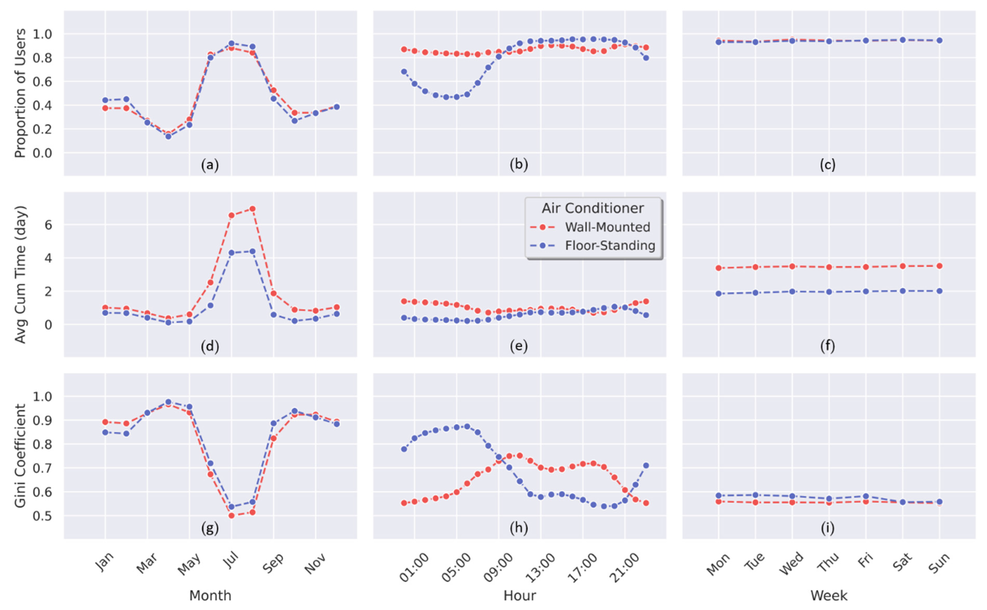
This section presents the classification of the Lower Class users and identifies the absolute poverty line of running time that satisfies the rigid demand of RAC use in a year. Firstly, the proportion of users with RAC in operation in total users at a certain period (Proportion of Users), the average cumulative running time (Avg. Cum. Time) and the Gini coefficient of running time (Gini Coefficient) are summarized by month, hour and week categories, as shown in Figure 3.

In the monthly category (Figure 3a,d,g), the Proportion of Users and the Avg. Cum. Time are the highest in June, July and August among the year, whereas the Gini Coefficient is the lowest. Among them, the difference in the Proportion of Users between bedroom cases and living-room cases is tiny. In contrast, the Avg. Cum. Time of bedroom cases is higher than that of living-room cases, especially in the summer. The Gini Coefficient of bedroom cases is slightly lower than that of living-room cases in summer but higher in winter. It reveals that the RAC demand was higher and more even in the summer period for bedroom cases and the winter period for living-room cases.

In the hourly category (Figure 3b,e,h), the Proportion of Users and the Avg. Cum. Time during daytime present little difference between bedroom cases and living-room cases, but a significant can be seen in the Proportion of Users at nights in living-room cases, which is also evidenced by the Gini coefficient. This indicates that the change trends of RAC demand during the day are different between bedroom and living-room cases. In the weekly category (Figure 3c,f,i), the Proportion of Users, the Avg. Cum. Time and the Gini Coefficient present no apparent difference between weekdays and weekends for both bedroom and living-room cases, indicating a little difference in RAC demand between weekdays and weekends between bedroom and living-room cases.

As mentioned above, the Gini Coefficient was sensitively consistent with the changes in RAC operation states (Proportion of Users and Avg. Cum. Time) on a monthly, hourly and weekly basis, and it is then used as an indicator to identify the inequality in RAC usage in this study.

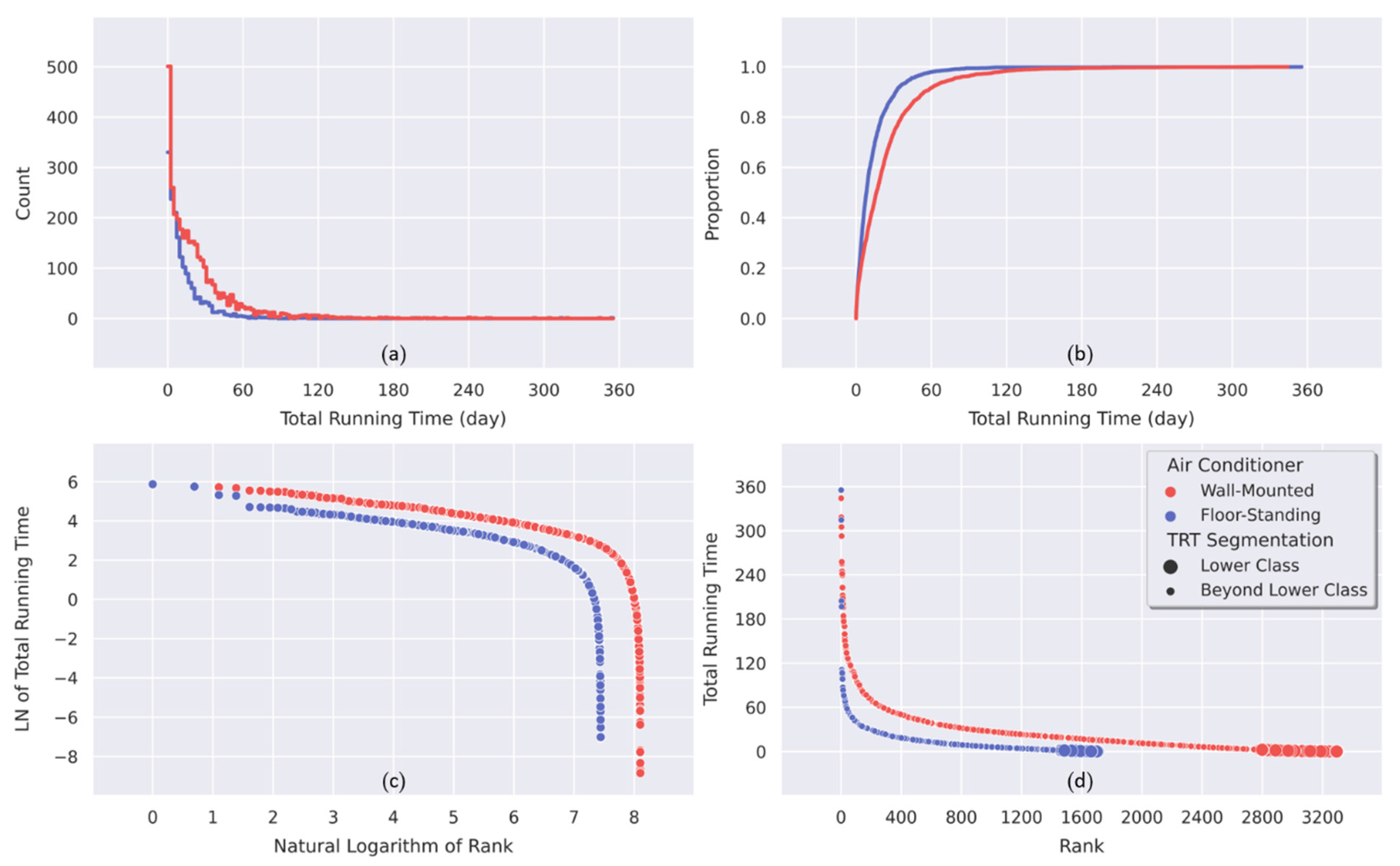
Figure 4a,b demonstrate the count and proportion of RAC running time data, suggesting an attenuation distribution, while Figure 4c demonstrates the existence of a piecewise distribution based on the log–log coordinate of rank size. To identify the Lower Class segmentation, the absolute poverty line was deduced for both bedroom and living-room cases and shown in Figure 4d. The absolute poverty line results in the large dots representing Lower Class users. Specifically, the annual running time in the Lower Class group is 2.53 and 1.71 days for bedroom and living-room cases, accounting for 15.67% and 15.10% of total users, respectively. It indicates that about 15% of RAC users in China’s HSCW zone operate RACs only to meet their rigid thermal demand annually.

3.2. Upper Class Segmentation

Based on the log–log coordinate of rank size, Figure 5(1-1) and Figure 6(1-1) presented the scaling region (large dots—excluding the Lower Class proportion) of bedroom and living-room cases. Due to the data distribution feature, the Lower Class part was omitted from the Upper Class classification process to improve the robustness. Outlier detection was conducted to detect cumulative errors in the data. Specifically, the error of heartbeat data loss, which describes the data loss due to incompatible action intervals and heartbeat time, was filtered and deleted by detecting the incomplete start and end time. Here, the algorithm Sn in Equation (6) was used to detect outliers (λ = 5), and the result of outlier detection is presented in the dark-red color in Figure 5(1-2), which accounts for 2.67% of the original data. Processed using the same method, the results of Upper Class segmentation in living-room cases are shown in Figure 6. The number of outliers accounted for 2.81% of the original data.

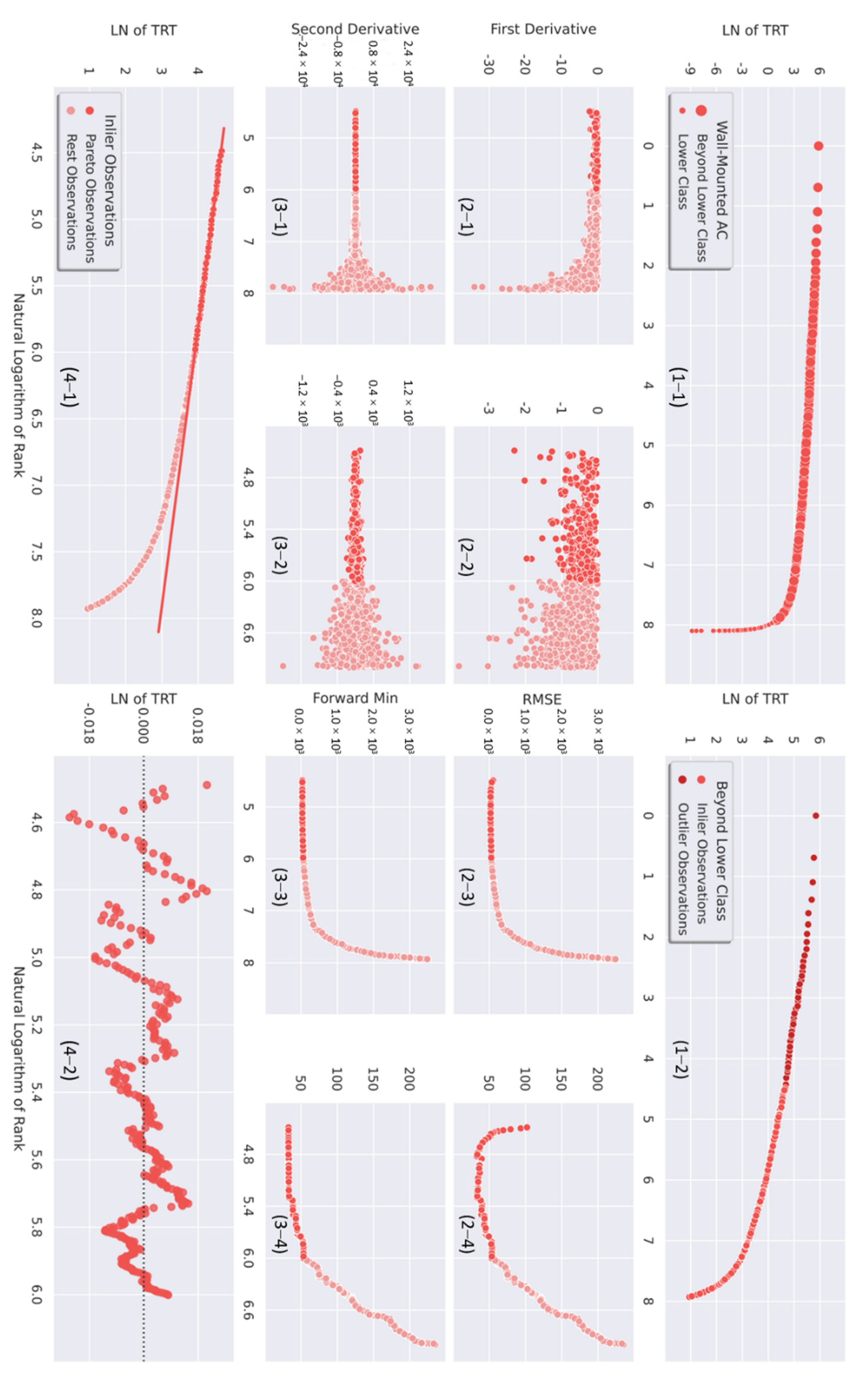
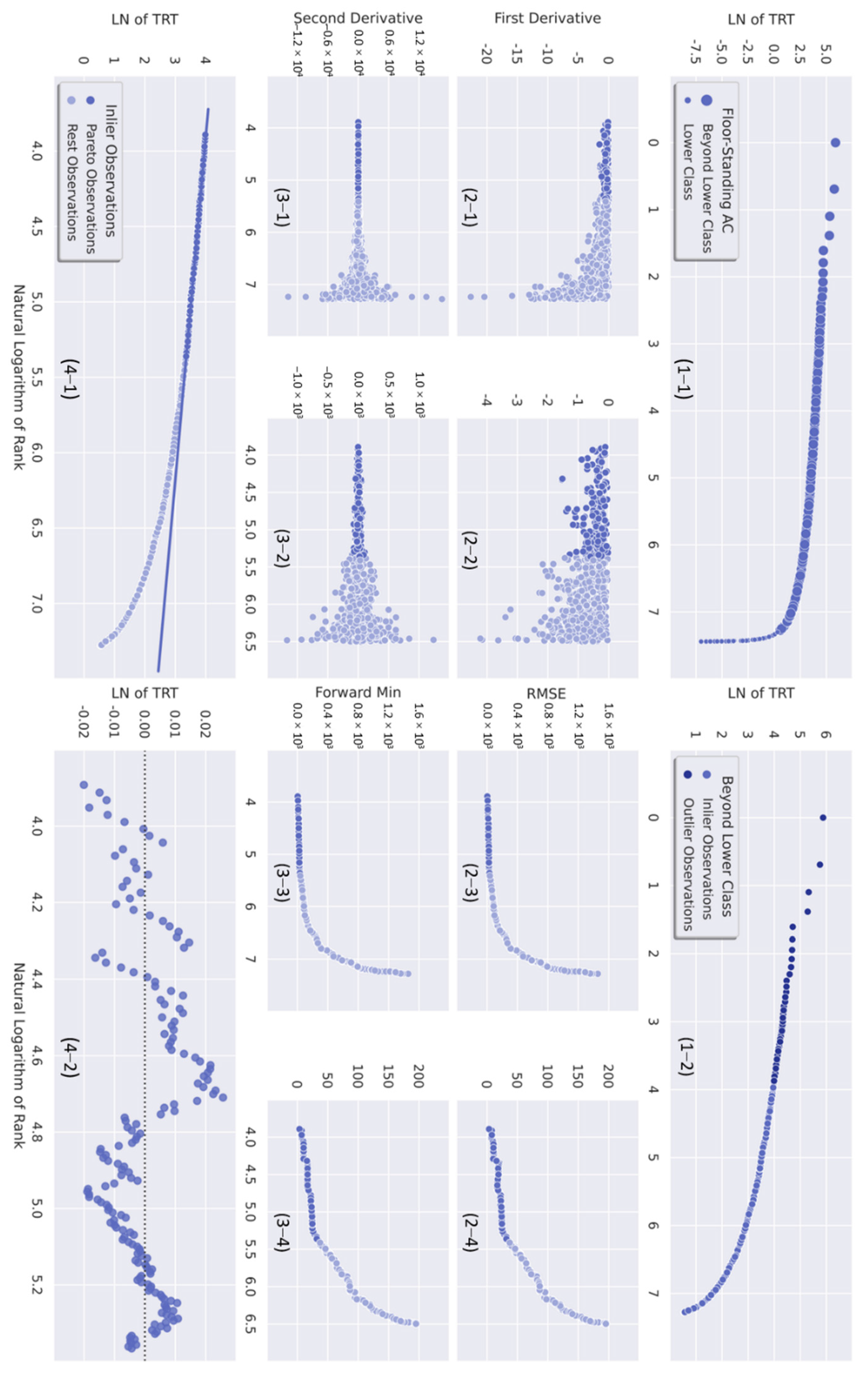
Based on the log–log coordinate of rank size, Figure 5(1-1) and Figure 6(1-1) presented the scaling region (large dots—excluding the Lower Class proportion) of bedroom and living-room cases. Due to the data distribution feature, the Lower Class part was omitted from the Upper Class classification process to improve the robustness. Outlier detection was conducted to detect cumulative errors in the data. Specifically, the error of heartbeat data loss, which describes the data loss due to incompatible action intervals and heartbeat time, was filtered and deleted by detecting the incomplete start and end time. Here, the algorithm Sn in Equation (6) was used to detect outliers (λ = 5), and the result of outlier detection is presented in the dark-red color in Figure 5(1-2), which accounts for 2.67% of the original data. Processed using the same method, the results of Upper Class segmentation in living-room cases are shown in Figure 6. The number of outliers accounted for 2.81% of the original data.

The scaling region was further derived by the second derivative method. The global and local first derivative (Figure 5(2-1),(2-2)) showed that the slope of the data trend changes greatly. The second derivative enlarged the data gap and provided a priori knowledge for predicting the straight-line segment $y=0$. As a result, the second derivative of the maximum linear segment was found to fluctuate slightly near 0, and the impact of low-ranking disturbances was greater than that of post-ranking disturbances. However, it might be hard to directly determine the maximum straight line nodes from the second derivative, as shown in Figure 5(3-1),(3-2).

Moreover, the RMSE analysis was also found to present a weak interpretation of distinguishing the segmenting points of the data, though the results implied the potential existence of the segment with a significant growth in the R² value, as shown in Figure 5(2-3),(2-4). Hence, the forward minimum algorithm (referring to Equation (6), $lnR=6.0$) was used to find out the maximum straight line, which contained the most data and the least disturbance, as demonstrated in Figure 5(3-3),(3-4).

Therefore, the scaling region of the power-law distribution was obtained by the data linear fitting, as shown in Figure 5(4-1). The regression equation was $y=-0.4772x+6.7738$, $r=-0.9993$, and the Upper Class accounted for 12.24% of the total RAC users. Figure 5(4-2) was the residual plot of linear fitting, which presented a sine function-like pattern around the fitting result. In Figure 6(4-1), the regression equation was $y=-0.4397x+5.7167$, $r=0.9985$, and the Upper Class accounted for 12.52% of the total RAC users.

To sum up, based on the results of Upper Class classification, the annual running time of the Upper Class group are 105.19 and 54.10 days for bedroom and living-room cases. The number of users that are categorized into the Upper Class group account for 12.26% and 12.52% of the total RAC users at the region, respectively. This implies that, based on the regional data examined in this study, about 12% of users in China’s HSCW zone belong to the Upper Class with high RAC usage demand, while the annual RAC running time of bedroom cases is twice longer than living-room cases.

3.3. Summary of RAC User Classification

This study segments RAC users as Lower and Upper Class groups, thus the proportion of Middle Class users reached 73%. In order to better observe the discrepancy of RAC usage demand among Middle Class users, they were divided into Lower Middle and Upper Middle Class groups by the average running time of Middle Class users. A discussion on the changing trends of four user groups would be presented in the next section. Figure 7 summarizes the results of RAC user classification by running time for bedroom and living-room cases. This study identified four RAC-user classes in the HSCW zone, including Lower/Lower Middle/Upper Middle/Upper Class, accounting for around 15%, 42%, 31% and 12% of the total RAC users, respectively, as shown in

Table 2. Class segmentation proportions in bedroom and living-room cases.

	Lower Class	Lower Middle Class	Upper Middle Class	Upper Class
Bedroom cases	15.67%	39.79%	32.30%	12.24%
Living-room cases	15.10%	43.12%	29.26%	12.52%

. The classification proportions present similar composition in bedroom and living-room cases, which might be a result of the consistency with the outdoor climates.

4. Discussion

This study proposed a method to classify users with distinct RAC demands at a regional level by using the indicator of RAC running time, and the method was applied to identify RAC user groups in China’s HSCW zone based on 196 million records from 5009 RACs. Based on the four class groups identified above, the RAC usage intensity and usage distribution of different classes and the implications and limitations of the classification are discussed in this section.

4.1. RAC Usage Intensity of Different User Classes

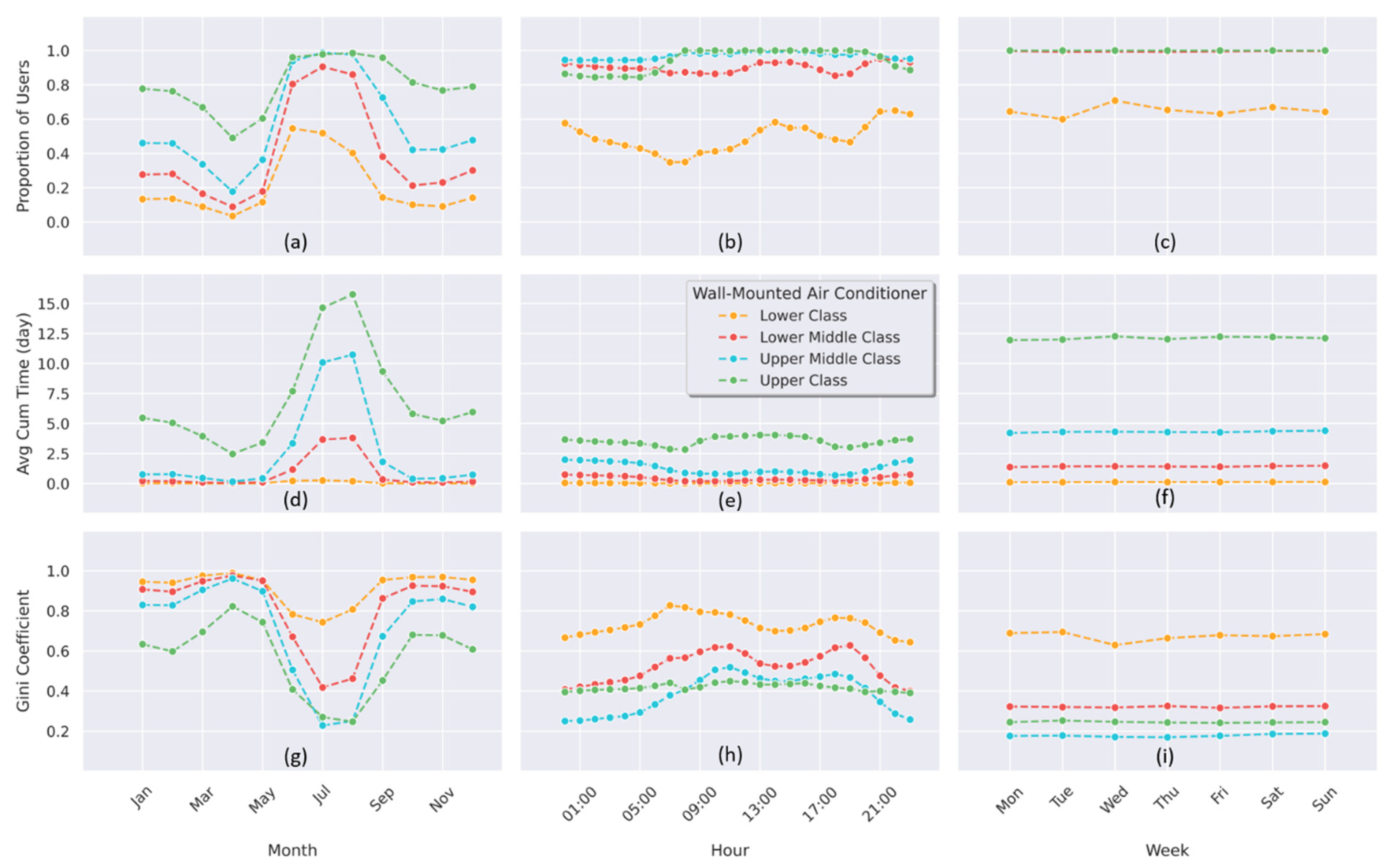
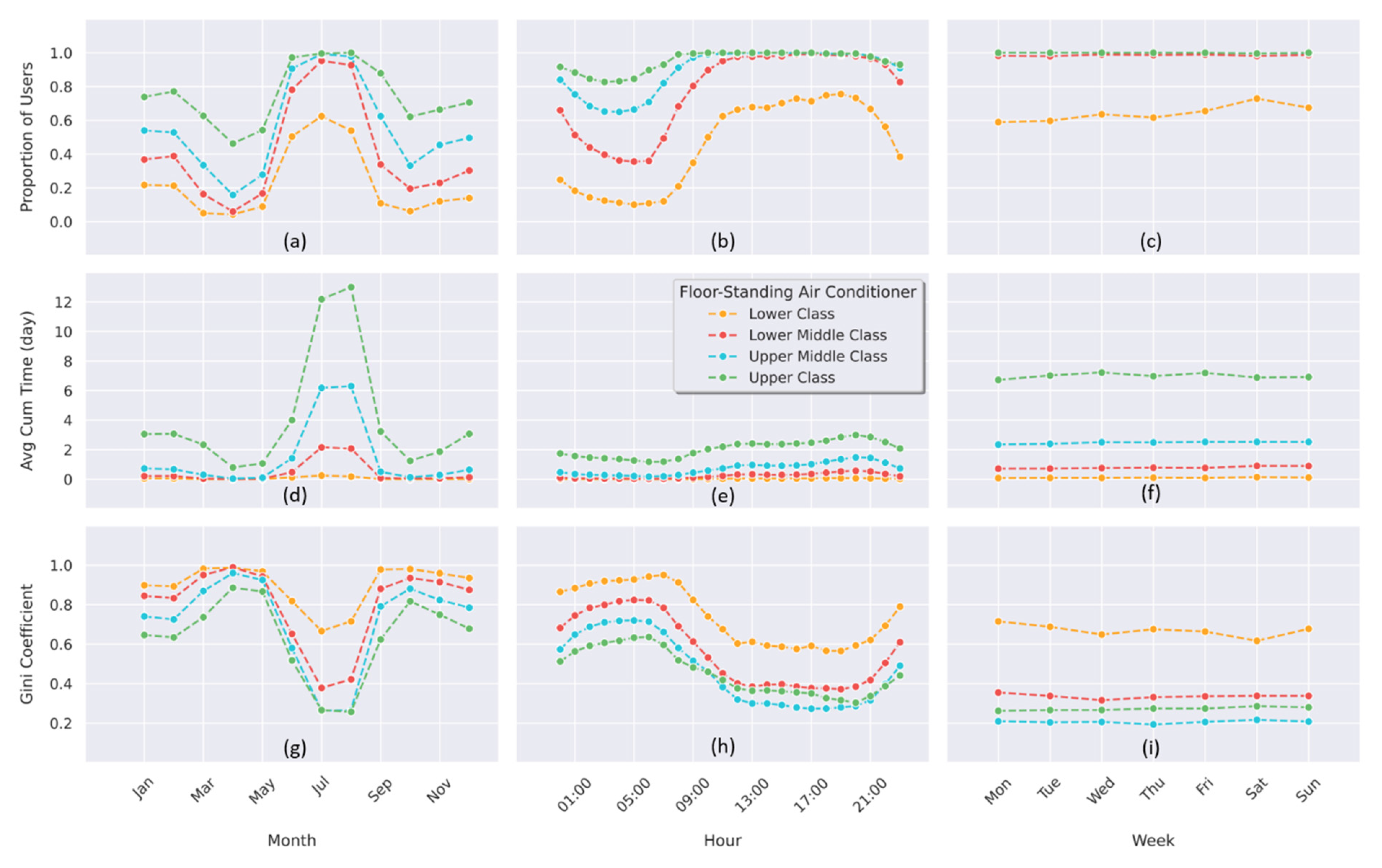
The usage intensities of four RAC user classes in bedroom and living-room cases are shown in Figure 8 and Figure 9, respectively.

The annual trends of running time in bedroom and living-room cases are similar, for example, RACs were used more in summer and winter seasons but less in transitional seasons, as shown in Figure 8a,d,g and Figure 9a,d,g. Meanwhile, RAC users in different user-class groups showed obvious differences in RAC usage demand during the winter season. It is also noted that some users in the Lower Class group only used their RACs in the summer period.

Moreover, the pattern of daily RAC use intensity varies between bedroom and living-room cases, as shown in Figure 8b,e,h and Figure 9b,e,h. Meanwhile, RAC users in four user-class groups experienced large differences in the RAC usage intensity at midnight. Interestingly, the RAC users in the Upper Class group who were supposed to use more RACs in daytime are found to use less RACs during the midnight in both bedroom and living-room cases. As shown in Figure 8b, the proportion of users in the Lower Class group was found to be higher at the midnight and noon but lower in morning and afternoon periods in bedroom cases. A similar result was also supported by An et al. [31] who found that the daily trend of turning on AC was consistent with Cluster 1 in the bedroom by clustering analysis.

However, three indicators presented fewer fluctuations weekly in both bedroom and living-room cases, as shown in Figure 8c,f,i and Figure 9c,f,i. Xia et al. [22] also reported little difference was found between the RAC operation rate in weekdays and weekends.

4.2. Usage Distribution of Different Classes

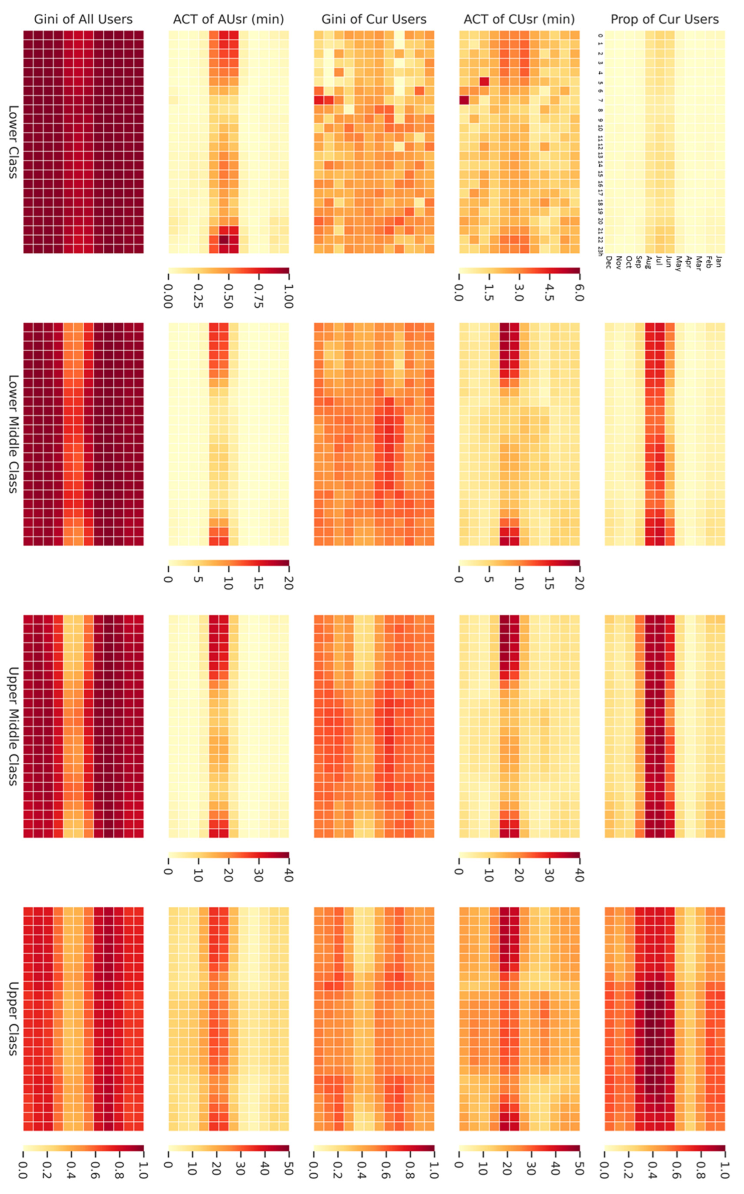
To compare the difference in the distribution features among four class groups, Figure 10 and Figure 11 illustrate the cross comparison of five RAC running-time indicators ($P_{cur}$ stands for proportion of current users, $T_{cur}$ is accumulated time of current users, $G_{cur}$ is Gini Coefficient of current users, $T_{all}$ is accumulated time of all users and $G_{all}$ is Gini Coefficient of all users) and four user groups (Lower/Lower Middle/Upper Middle/Upper Class) in monthly and hourly periods. In the heatmaps, each time grid represents the indicator in the sum of a specific hour (horizontal axis) of a given month (vertical axis). The darker the color of the grid, the greater the value. Generally, the color of grids becomes darker from Lower Class category to Upper Class category regarding the proportion of current users, accumulated time of current users, Gini Coefficient of current users and the accumulated time of all users.

To clarify the similarities and differences in RAC operation demand among user-class groups in bedroom and living-room cases,

Table 3. The maximal and minimal values of five indicators in different periods.

	${\mathit{P}}_{\mathit{c}\mathit{u}\mathit{r}}$		${\mathit{T}}_{\mathit{c}\mathit{u}\mathit{r}}$		${\mathit{G}}_{\mathit{c}\mathit{u}\mathit{r}}$		${\mathit{T}}_{\mathit{a}\mathit{l}\mathit{l}}$		${\mathit{G}}_{\mathit{a}\mathit{l}\mathit{l}}$
	Max	Min	Max	Min	Max	Min	Max	Min	Max	Min
	Bedroom cases
Lower Class	S-E	T-N	S-N	T-D	S-E	T-N	S-N	T-N	T-N	S-N
Lower Middle Class	S-N	T-N	S-N	T-N	T-D	T-N	S-N	T-N	T-D	S-N
Upper Middle Class	S-N	T-D	S-N	T-E	T-D	S-N	S-N	T-N	T-D	S-N
Upper Class	S-D	T-N	S-N	T-E	T-E	S-N	S-N	T-N	T-N	S-N
	Living-room cases
Lower Class	S-E	T-N	S-N	T-N	S-D	T-N	S-E	T-N	S-N	T-N
Lower Middle Class	S-E	T-N	S-E	T-D	T-E	T-N	S-E	T-N	T-N	S-E
Upper Middle Class	S-E	T-N	S-E	T-N	T-D	T-N	S-E	T-N	T-N	S-E
Upper Class	S-E	T-N	S-E	T-D	T-D	S-E	S-E	T-N	T-N	S-N

summarizes the seasonal periods with the maximal and minimal values of the five running-time indicators (“S” stands for summer season from June to September, “W” stands for winter season from December to February and “T” stands for a transitional season with other months) and periods (“D” stands for daytime from 7:00 to 18:00, “E” stands for evening from 19:00 to 22:00 and “N” stands for night from 23:00 to 06:00). For example, “S-W” means summer daytime, that is 7:00–18:00 in June to September.

In summary, the rigid demand of Lower Class users was concentrated in summer nights in bedroom cases, while users in other classes had the longest accumulated time during summer nights. Meanwhile, the RAC demand in summer daytime was limited in Lower Class users. Furthermore, increasing RAC usage was observed from Lower Class group to Upper Class groups in summer daytime. In living-room cases, the distribution of RAC usage demand was similar among the four user-class groups. The period with the highest proportion of users was found in summer evenings, while the lowest value was found in transitional nights. The longest accumulated time of RAC operation was found in summer evenings except for in the Lower Class group, where the longest accumulated time was in summer nights.

4.3. Implications for Regional Energy Management

RAC running time has been proven in this study to represent the overall trend of RAC power consumption and usage demand in China’s HSCW zone. At the regional level, the novelty of this study is that it proposes a method of classification of different user groups with different energy usage demands based on a single index—the running time of RACs—and examines the difference between rigid and flexible demand. This classification method can also be utilized in other regions. As the global temperature rose this year, the global power load of RACs increased during the summer. For example, this method could be used for regional energy regulation in European countries. In addition, the running time of other energy supply systems besides RACs can be taken into account, such as the energy usage demand of winter heating systems.

The RAC operation periods identified for satisfying rigid demand in the Lower Class group can hardly be reduced, as the further reduction might affect people’s rigid thermal comfort expectation and the living quality of avoiding excessive warmth and coldness. Moreover, the Upper Class group was identified with flexible RAC operation periods and could be used to determine the schedulable time window for the purpose of building energy flexibility management. As mentioned in Section 4.2, the monthly periods of rigid RAC demand are June, July and August. In bedroom cases, the hourly periods of rigid demand are 21:00–6:00. In living-room cases, the hourly periods of rigid demand are 11:00–22:00. Hence, 21:00–22:00 is the overlapping hourly period of rigid demand for both bedroom and living-room cases. Therefore, securing the regional power load during 21:00–22:00 in summers is crucial for maintaining the rigid living comfort of RAC users. Based on the RAC running time at the regional level, this study suggests the regional power supply should satisfy the RAC running period for rigid demand and then attempt to exploit the energy flexibility potential in the period with flexible demand.

The flexible energy of a building/buildings is an active area in terms of demand-side response, it is defined as single or cluster of buildings able to manage the energy demand with consideration of local climate conditions, user needs and grid requirements in IEA Annex 67 [55]. In order to better manage the energy demand of household RACs, the flexible demand of RAC can be understood as RAC usage that can be be shifted or shed or modulated. To explore the flexibility potential of each class group, the unit demand of running time-based RAC is calculated in Equation (7).

$$D_{unit}=\frac{T_{max}}{C_{avg}}$$

(7)

where $D_{unit}$ is unit demand of each class, $T_{max}$ is the max anuual running time of each class and $C_{avg}$ is the average capacity of each class. Generally, the capacities of RACs in bedroom cases comprise 2.6 kW/3.2 kW/3.5 kW and the capacities in living-room cases comprise 5.1 kW/7.2 kW.

The results of Equation (7) are listed in

Table 4. Unit demand of different classes in bedroom and living-room cases.

Unit Demand (h/kw)	Lower Class	Lower Middle Class	Upper Middle Class	Upper Class
Bedroom cases	19.78	149.33	384.31	2533.84
Living-room cases	6.46	39.36	109.73	1366.5

. The rigid unit demand (Lower Class) is 19.78 h/kw (bedroom cases) and 6.46 h/kw (living-room cases). In bedroom cases, the flexible unit demands of Lower Middle/Upper Middle/Upper Class are 7.55/19.42/128.10 times that of the rigid unit demand. In addition, in living-room cases, the flexible unit demands of Lower Middle/Upper Middle/Upper Class are 6.09/16.99/211.53 times that of rigid unit demand. Similar findings of flexibility, such as delayed flexibility and forced flexibility that based on the 24-h day can also be seen in Chen et al. [10]. In general, the flexibility potential increases gradually from Lower to Upper Class. In Middle Class, the flexibility potential of bedroom and living-room cases is similar. However, the flexibility potential of the living room cases is twice that of the bedroom cases in the Upper Class. The Upper Class users account for a small proportion but dominate extremely high RAC running time. The reason may be that this group has unique RAC preference and a high usage demand. So, the flexibility potential of the Upper Class needs further study, although their unit demand value is the highest.

4.4. Limitations

The samples in the database are from China’s HSCW zone. The buildings used as samples were all constructed after 2005, and their energy-saving design standards in China are consistent. Therefore, the analysis results are less affected in this study by climate, building age and occupant heat condition. However, the main limitation of this study is that the warehouse data were collected in three cities in China’s HSCW zone. The results might not be applicable for other regions; however, the method proposed by this study can be adopted as a reference to identify user group class in other regions. Moreover, the raw dataset contains missing values within a certain period. Although different protocols were combined to restore the data, there may be inevitable systematic errors. A further investigation on the analysis of behavior patterns is recommended in order to further reveal the interrelationship between behavior patterns and user classes.

5. Conclusions

By adopting the data-driven method and using running time as an indicator, this study classifies the household RAC user groups and identifies the RAC usage demand of households in hot summer and cold winter zone of China. A total of 196 million annual real-time tracking records from 5009 household RACs were extracted from the database in three representative cities (Chongqing, Wuhan and Shanghai) in the HSCW zone of China. The main conclusions are summarized as follows:

• This study proposes data-driven methods to classify RAC user groups by running time over a year at regional level from novel perspectives. On the one hand, a few RAC users in the Lower Class, which is identified by the absolute poverty line with the Gini coefficient of annual running time distribution. On the other hand, a small number of the Upper Class group is distinguished through the determination of the scaling region in the power-law distribution.
• Based on the case study in the HSCW zone of China, the annual trends of running times in bedroom and living-room cases are similar, thus the Lower/Lower Middle/Upper Middle/Upper Class groups account for around 15%/42%/31%/12% of the total RAC users, respectively. In general, the flexibility potential increases gradually from Lower to Upper Class.
• Among all classes, RACs are used more in summer and winter seasons but less in transitional seasons. Meanwhile, RAC users in different user-class groups show obvious differences in usage demand in the winter season. Overall, the summer season has the most RAC monthly rigid demand periods over the year, both in bedroom and living-room cases.
• The patterns of daily RAC use intensity of four classes are different between bedroom and living-room cases, especially in midnight. In addition, 21:00–22:00 is the overlapping hourly rigid demand period for both bedroom and living-room cases.

References

1. BERC. Annual Report on China Building Energy Efficiency; Tsinghua University: Beijing, China, 2020. [Google Scholar]
2. Sha, H.; Xu, P.; Hu, C.; Li, Z.; Chen, Y.; Chen, Z. A simplified HVAC energy prediction method based on degree-day. Sustain. Cities Soc. 2019, 51, 101698. [Google Scholar] [CrossRef]
3. Yan, D.; O’Brien, W.; Hong, T.; Feng, X.; Burak Gunay, H.; Tahmasebi, F.; Mahdavi, A. Occupant behavior modeling for building performance simulation: Current state and future challenges. Energy Build. 2015, 107, 264–278. [Google Scholar] [CrossRef]
4. Hu, S.; Yan, D.; Guo, S.; Cui, Y.; Dong, B. A survey on energy consumption and energy usage behavior of households and residential building in urban China. Energy Build. 2017, 148, 366–378. [Google Scholar] [CrossRef]
5. Hu, S.; Yan, D.; Qian, M. Using bottom-up model to analyze cooling energy consumption in China’s urban residential building. Energy Build. 2019, 202, 109352. [Google Scholar] [CrossRef]
6. National Bureau of Statistics of China. China Statistical Yearbook; China Statistics Press: Beijing, China, 2020. Available online: http://www.stats.gov.cn/tjsj/ndsj/2020/indexch.htm (accessed on 30 July 2022).
7. Feng, X.; Yan, D.; Wang, C.; Sun, H. A preliminary research on the derivation of typical occupant behavior based on large-scale questionnaire surveys. Energy Build. 2016, 117, 332–340. [Google Scholar] [CrossRef]
8. Qi, N.; Cheng, L.; Xu, H.; Wu, K.; Li, X.L.; Wang, Y.; Liu, R. Smart meter data-driven evaluation of operational demand response potential of residential air conditioning loads. Appl. Energy 2020, 279, 115708. [Google Scholar] [CrossRef]
9. Sena, B.; Zaki, S.A.; Rijal, H.B.; Ardila-Rey, J.A.; Yusoff, N.M.; Yakub, F.; Ridwan, M.K.; Muhammad-Sukki, F. Determinant factors of electricity consumption for a Malaysian household based on a field survey. Sustainability 2021, 13, 818. [Google Scholar] [CrossRef]
10. Chen, Y.; Xu, P.; Gu, J.; Schmidt, F.; Li, W. Measures to improve energy demand flexibility in buildings for demand response (DR): A review. Energy Build. 2018, 177, 125–139. [Google Scholar] [CrossRef]
11. Newsham, G.R.; Birt, B.J.; Rowlands, I.H. A comparison of four methods to evaluate the effect of a utility residential air-conditioner load control program on peak electricity use. Energy Policy 2011, 39, 6376–6389. [Google Scholar] [CrossRef]
12. Li, W.; Xu, P. A fast method to predict the demand response peak load reductions of commercial buildings. Sci. Technol. Built Environ. 2016, 22, 633–642. [Google Scholar] [CrossRef]
13. Sehar, F.; Pipattanasomporn, M.; Rahman, S. An energy management model to study energy and peak power savings from PV and storage in demand responsive buildings. Appl. Energy 2016, 173, 406–417. [Google Scholar] [CrossRef]
14. Reynders, G.; Amaral Lopes, R.; Marszal-Pomianowska, A.; Aelenei, D.; Martins, J.; Saelens, D. Energy flexible buildings: An evaluation of definitions and quantification methodologies applied to thermal storage. Energy Build. 2018, 166, 372–390. [Google Scholar] [CrossRef]
15. Olawale, O.W.; Gilbert, B.; Reyna, J. Residential Demand Flexibility: Modeling Occupant Behavior using Sociodemographic Predictors. Energy Build. 2022, 262, 111973. [Google Scholar] [CrossRef]
16. Yan, L.; Liu, M. A simplified prediction model for energy use of air conditioner in residential buildings based on monitoring data from the cloud platform. Sustain. Cities Soc. 2020, 60, 102194. [Google Scholar] [CrossRef]
17. Ren, G.; Sunikka-Blank, M.; Zhang, X. Young urban households in Shanghai, China: Characteristics of energy use and attitudes. Sustain. Cities Soc. 2020, 60, 102174. [Google Scholar] [CrossRef]
18. Xue, K.; Liu, M.; Ma, M.; Hu, M.; Yan, L.; Chen, X.; Zeng, W. A framework for short-term energy consumption prediction based on room air conditioner group characteristics. J. Build. Eng. 2021, 52, 104400. [Google Scholar] [CrossRef]
19. Malik, A.; Haghdadi, N.; MacGill, I.; Ravishankar, J. Appliance level data analysis of summer demand reduction potential from residential air conditioner control. Appl. Energy 2019, 235, 776–785. [Google Scholar] [CrossRef]
20. Ren, X.; Yan, D.; Wang, C. Air-conditioning usage conditional probability model for residential buildings. Build. Environ. 2014, 81, 172–182. [Google Scholar] [CrossRef]
21. Yao, J. Modelling and simulating occupant behaviour on air conditioning in residential buildings. Energy Build. 2018, 175, 1–10. [Google Scholar] [CrossRef]
22. Xia, D.; Lou, S.; Huang, Y.; Zhao, Y.; Li, D.H.W.; Zhou, X. A study on occupant behaviour related to air-conditioning usage in residential buildings. Energy Build. 2019, 203, 109446. [Google Scholar] [CrossRef]
23. Xu, X.; Liu, W.; Lian, Z. Dynamic indoor comfort temperature settings based on the variation in clothing insulation and its energy-saving potential for an air-conditioning system. Energy Build. 2020, 220, 110086. [Google Scholar] [CrossRef]
24. Mariano-Hernández, D.; Hernández-Callejo, L.; Zorita-Lamadrid, A.; Duque-Pérez, O.; Garcia, F.S. A review of strategies for building energy management system: Model predictive control, demand side management, optimization, and fault detect & diagnosis. J. Build. Eng. 2021, 33, 101692. [Google Scholar]
25. Pandey, B.; Bohara, B.; Pungaliya, R.; Patwardhan, S.C.; Banerjee, R. A thermal comfort-driven model predictive controller for residential split air conditioner. J. Build. Eng. 2021, 42, 102513. [Google Scholar] [CrossRef]
26. Liu, H.; Sun, H.; Mo, H.; Liu, J. Analysis and modeling of air conditioner usage behavior in residential buildings using monitoring data during hot and humid season. Energy Build. 2021, 250, 111297. [Google Scholar] [CrossRef]
27. Yan, L.; Liu, M. Predicting household air conditioners’ on/off state considering occupants’ preference diversity: A study in Chongqing, China. Energy Build. 2021, 253, 111516. [Google Scholar] [CrossRef]
28. Tran, L.N.; Gao, W.; Ge, J. Sensitivity analysis of household factors and energy consumption in residential houses: A multi-dimensional hybrid approach using energy monitoring and modeling. Energy Build. 2021, 239, 110864. [Google Scholar] [CrossRef]
29. Ouyang, J.; Hokao, K. Energy-saving potential by improving occupants’ behavior in urban residential sector in Hangzhou City, China. Energy Build. 2009, 41, 711–720. [Google Scholar] [CrossRef]
30. Rinaldi, A.; Schweiker, M.; Iannone, F. On uses of energy in buildings: Extracting influencing factors of occupant behaviour by means of a questionnaire survey. Energy Build. 2018, 168, 298–308. [Google Scholar] [CrossRef]
31. An, J.; Yan, D.; Hong, T. Clustering and statistical analyses of air-conditioning intensity and use patterns in residential buildings. Energy Build. 2018, 174, 214–227. [Google Scholar] [CrossRef]
32. Kindaichi, S.; Nishina, D.; Murakawa, S.; Ishida, M.; Ando, M. Analysis of energy consumption of room air conditioners: An approach using individual operation data from field measurements. Appl. Therm. Eng. 2017, 112, 7–14. [Google Scholar] [CrossRef]
33. Zhou, X.; Yan, D.; Feng, X.; Deng, G.; Jian, Y.; Jiang, Y. Influence of household air-conditioning use modes on the energy performance of residential district cooling systems. Build. Simul. 2016, 9, 429–441. [Google Scholar] [CrossRef]
34. Sun, Y.; Haghighat, F.; Fung, B.C.M. A review of the-state-of-the-art in data-driven approaches for building energy prediction. Energy Build. 2020, 221, 110022. [Google Scholar] [CrossRef]
35. Du, J.; Pan, W.; Yu, C. In-situ monitoring of occupant behavior in residential buildings—A timely review. Energy Build. 2020, 212, 109811. [Google Scholar] [CrossRef]
36. NOAA. NOAA National Centers for Environmental Information (2001): Global Surface Hourly [57516099999, 57494099999 and 58362099999]. Available online: https://www.ncei.noaa.gov/access/search/data-search/global-hourly?stations= (accessed on 31 July 2022).
37. Robinson, C.; Yan, D.; Bouzarovski, S.; Zhang, Y. Energy poverty and thermal comfort in northern urban China: A household-scale typology of infrastructural inequalities. Energy Build. 2018, 177, 363–374. [Google Scholar] [CrossRef]
38. Thomson, H.; Simcock, N.; Bouzarovski, S.; Petrova, S. Energy poverty and indoor cooling: An overlooked issue in Europe. Energy Build. 2019, 196, 21–29. [Google Scholar] [CrossRef]
39. van Hove, W.; Dalla Longa, F.; van der Zwaan, B. Identifying predictors for energy poverty in Europe using machine learning. Energy Build. 2022, 264, 112064. [Google Scholar] [CrossRef]
40. Ravallion, M. Poverty lines. In The New Palgrave Dictionary of Economics; Palgrave Macmillan: London, UK, 2008; p. 2. [Google Scholar]
41. Milanovic, B. A simple way to calculate the Gini coefficient, and some implications. Econ. Lett. 1997, 56, 45–49. [Google Scholar] [CrossRef]
42. Jacobson, A.; Milman, A.D.; Kammen, D.M. Letting the (energy) Gini out of the bottle: Lorenz curves of cumulative electricity consumption and Gini coefficients as metrics of energy distribution and equity. Energy Policy 2005, 33, 1825–1832. [Google Scholar] [CrossRef]
43. Sitthiyot, T.; Holasut, K. A simple method for measuring inequality. Palgrave Commun. 2020, 6, 112. [Google Scholar] [CrossRef]
44. Leys, C.; Ley, C.; Klein, O.; Bernard, P.; Licata, L. Detecting outliers: Do not use standard deviation around the mean, use absolute deviation around the median. J. Exp. Soc. Psychol. 2013, 49, 764–766. [Google Scholar] [CrossRef]
45. Reed, G.F.; Lynn, F.; Meade, B.D. Use of coefficient of variation in assessing variability of quantitative assays. Clin. Diagn. Lab. Immunol. 2002, 9, 1235–1239. [Google Scholar] [CrossRef] [Green Version]
46. Newman, M.E.J. The structure and function of complex networks. SIAM Rev. 2003, 45, 167–256. [Google Scholar] [CrossRef]
47. OliveiraJG, B. Humandynamics: Darwin and einstein correspondence patterns. Nature 2005, 437, 1251r1253. [Google Scholar]
48. Zhao, Z.-D.; Zhou, T. Empirical analysis of online human dynamics. Phys. A Stat. Mech. Its Appl. 2012, 391, 3308–3315. [Google Scholar] [CrossRef]
49. Yang, T.; Feng, X.; Wu, Y.; Wang, S.; Xiao, J. Human dynamics in repurchase behavior based on comments mining. Phys. A Stat. Mech. Its Appl. 2018, 502, 563–569. [Google Scholar] [CrossRef]
50. Rousseeuw, P.J.; Croux, C. Alternatives to the median absolute deviation. J. Am. Stat. Assoc. 1993, 88, 1273–1283. [Google Scholar] [CrossRef]
51. Cousineau, D.; Chartier, S. Outliers detection and treatment: A review. Int. J. Psychol. Res. 2010, 3, 58–67. [Google Scholar] [CrossRef]
52. Jones, P.R. A note on detecting statistical outliers in psychophysical data. Atten. Percept. Psychophy 2019, 81, 1189–1196. [Google Scholar] [CrossRef]
53. Clauset, A.; Shalizi, C.R.; Newman, M.E.J. Power-Law Distributions in Empirical Data. SIAM Rev. 2009, 51, 661–703. [Google Scholar] [CrossRef]
54. Wang, C.; Ling, D.; Miao, Q. Automatic identification method of fractal scaling region. Eng. Appl. 2012, 48, 9–12. [Google Scholar]
55. O’Brien, W.; Wagner, A.; Schweiker, M.; Mahdavi, A.; Day, J.; Kjærgaard, M.B.; Carlucci, S.; Dong, B.; Tahmasebi, F.; Yan, D.; et al. Introducing IEA EBC Annex 79: Key challenges and opportunities in the field of occupant-centric building design and operation. Build. Environ. 2020, 178, 106738. [Google Scholar] [CrossRef]
Figure 1. The framework to classify household RAC user groups by running time.
Buildings 12 01415 g001
Figure 2. Distribution and relationship among YRT, MTD and TPC in effective power samples.
Buildings 12 01415 g002
Figure 3. The relationship of the proportion of users, average cumulative time and Gini coefficient in bedroom and living-room cases. (a) monthly proportion of users; (b) hourly proportion of users; (c) weekly proportion of users; (d) monthly average cumulative time; (e) hourly average cumulative time; (f) weekly average cumulative time; (g) monthly Gini coefficient; (h) hourly Gini coefficient; (i) weekly Gini coefficient.
Buildings 12 01415 g003
Figure 4. Lower Class segmentation of running time in bedroom and living-room cases. (a) histogram, (b) CDF, (c) log–log coordinate of rank-size and (d) Lower Class.
Buildings 12 01415 g004
Figure 5. Process of Upper Class segmentation in bedroom cases, (1-1) beyond Lower Class, (1-2) outlier detection, (2-1) global first derivative, (2-2) local first derivative, (2-3) global RMSE, (2-4) local RMSE, (3-1) global second derivative, (3-2) local second derivative, (3-3) global forward min, (3-4) local forward min, (4-1) linear regression pareto segmentation and (4-2) residual plot.
Buildings 12 01415 g005
Figure 6. Process of Upper Class segmentation in living-room cases (the subgraphs are consistent with Figure 5).
Buildings 12 01415 g006
Figure 7. Class segmentation results in bedroom and living-room cases.
Buildings 12 01415 g007
Figure 8. Comparison of four classes in RAC users in bedroom cases. (a) monthly proportion of users; (b) hourly proportion of users; (c) weekly proportion of users; (d) monthly average cumulative time; (e) hourly average cumulative time; (f) weekly average cumu-lative time; (g) monthly Gini coefficient; (h) hourly Gini coefficient; (i) weekly Gini coefficient.
Buildings 12 01415 g008
Figure 9. Comparison of four classes in RAC users in living-room cases. (a) monthly proportion of users; (b) hourly proportion of users; (c) weekly proportion of users; (d) monthly average cumulative time; (e) hourly average cumulative time; (f) weekly average cumu-lative time; (g) monthly Gini coefficient; (h) hourly Gini coefficient; (i) weekly Gini coefficient.
Buildings 12 01415 g009
Figure 10. Heatmap of usage distribution of different classes in bedroom cases.
Buildings 12 01415 g010
Figure 11. Heatmap of usage distribution of different classes in living-room cases.
Buildings 12 01415 g011