Comparative Analysis between Genetic Algorithm and Simulated Annealing-Based Frameworks for Optimal Sensor Placement and Structural Health Monitoring Purposes

Abstract

The arbitrary placement of sensors in concrete structures measures a considerable amount of unnecessary data. Optimal sensor placement methods are used to provide informative data with the least cost and maximum efficiency. In this study, a robust optimal sensor placement framework that combines an optimization-based algorithm, the simulated annealing (SA) algorithm, and the ensemble Kalman filter (EnKF) are presented for structural health monitoring and system identification. The SA algorithm randomly generates an initial population of sensor locations, while the framework undergoes a minimization process. The objective function used is the difference between the actual measured data and their corresponding EnKF predicted values. A comparative analysis between the genetic algorithm–ensemble Kalman filter (GA-EnKF) and the simulated annealing–ensemble Kalman filter (SA-EnKF) approaches is presented. The performance and computational burden of both algorithms, which converge to the best sensor locations for damage detection purposes, are tested on a 10-story building subjected to a seismic excitation. The results are compared to the optimal sensor locations of the brute-force search methodology. The GA-EnKF outperforms the SA-EnKF in terms of accuracy in converging to the optimal results, yet the computational cost of the SA-EnKF is considerably lower.

1. Introduction

The deployment of innovative sensors and monitoring devices in concrete structures has made structural health monitoring (SHM) techniques more advanced and the early damage detection process easier [1]. Due to the massive advancement in the field of monitoring instruments and global positioning systems, the problem of analyzing and processing large flows of online SHM measurement data has arisen [2]. Thus, the optimal sensors configuration of the instrumented structure should be secured to extract the fundamental and informative data for damage detection.

Numerous optimal sensor placement (OSP) methods, including optimization-based and selection-based techniques, were proposed in the literature to determine the best sensor locations for damage detection and structural health monitoring purposes. The genetic algorithm (GA) approach was applied by many researchers for the purpose of optimal sensor placement. Guo et al. [1] suggested an alteration in the crossover and mutation operations to improve the GA approach and applied this upgraded version of the GA to identify the optimal sensor locations of a two-dimensional (2D) truss framework. Sebt et al. [3] applied the GA methodology to determine the best locations and characteristics of TADAS dampers in steel-moment-resisting frame (SMRF) structures. Two numerical examples were presented in this study, i.e., six-story and a ten-story moment-resisting steel structures equipped with TADAS dampers and subjected to a severe earthquake. Abbasi et al. [4] suggested a genetic algorithm-based approach to optimally place seismic vibration control actuators and determine their optimum numbers. The authors tested the proposed framework on a nonlinear 20-story benchmark building. Downey et al. [5] formulated a multi-objective optimization function to reduce type I and II errors in SHM systems and presented an adaptive mutation-based genetic algorithm for optimal sensor placement within a hybrid dense sensor network (HDSN). Hou et al. [6] proposed a GA-based optimal sensor placement technique for L1-regularized damage detection. In this study, the fitness function to be minimized was taken to be the mutual coherence of the sensitivity matrix. The authors validated the efficiency and robustness of their suggested framework on an experimental cantilever beam and a three-story frame. Su et al. [7] recently presented an optimal accelerometers placement method based on a partitioned genetic algorithm procedure for monitoring a high-piled wharf structure. The efficacy and validity of the proposed strategy was tested on a reduced-scale model of a high-piled wharf.

Several studies suggested combinations between the GA framework and the Bayesian approach for optimal sensor placement purposes. In these studies, the Bayesian approach starts by quantifying the parameters’ uncertainties and the GA then minimizes the information entropy over the set of probable sensor positions. Papadimitriou et al. [8] applied this combinatorial approach on two numerical examples, a nine-story building and a 29-degrees-of-freedom (DOF) truss framework, to determine the best scheme for the sensors. Flynn et al. [9] used the same methodology and applied it in the field of active sensing to identify the best locations for the sensors. Chow et al. [10] used the same approach to identify the optimal configuration for sensors of a three-dimensional (3D) finite element model of a transmission tower. Ponticelli et al. [11] suggested an optimization model based on the GA approach to control the fatigue life of AISI 1040 medium carbon steel after a diode laser-hardening process. It was shown that the proposed genetic algorithm-based methodology rapidly converged to the optimal regression model [12,13].

Besides the GA approach, the simulated annealing (SA) approach has been extensively used by many researchers for optimal sensor placement purpose. In their study, Chiu and Lin [14,15] focused on determining the sensor placement for a target location with full coverage at a limited cost. The authors used the SA algorithm to determine the optimal locations of sensors and tested the accuracy of the framework on two examples of sensor fields. The first example consisted of a small regular rectangular sensor field of 30 grid points only and the second example comprised two larger sensor fields with 10 × 10 and 30 × 30 grid points. Tong et al. [16] introduced an improved SA algorithm to determine the best sensor locations. The proposed method was established to search in additional dimensions and consequently increase the random search performance with minimum computational burden. The robustness of the algorithm is tested on a numerical problem consisting of a slab model using three types of fitness functions: the determinant of the Fisher information matrix (FIM), the modal assurance criterion (MAC) and the mean square error (MSE) of the mode shapes. Leitold et al. [17] recently proposed two clustering and simulated annealing-based methodologies—the clustering large applications based on the SA algorithm (CLASA) and the geodesic distance-based fuzzy c-medoid clustering method (GDFCM)—to control the locations of the additional sensors implemented due to the large size of the system.

Several research papers presented comparative studies between different heuristic methods, mainly the GA, the SA, and the Tabu Search (TS) frameworks. Augugliaro et al. [18] presented a comparison between the three previously mentioned optimization-based methods for OSP purpose. The minimization procedure was based on the power loss. The results show that TS is the most efficient method, whereas the GA approach outperforms the SA technique. Hasan et al. [19] compared the same three heuristic approaches and conducted three different solutions for the unconstrained quadratic pseudo-boolean (QP) function. The results show that the GA presented the best solutions in the least computational time. On the other hand, The SA algorithm outperformed the TS method. Arostegui et al. [20] conducted a comparative analysis between these three approaches to solve three variations in the facility location problems (FLP): The capacitated FLP (CFLP), the multi-period FLP (MPFLP), and the multi-commodity FLP (MCFLP). For the CFLP problem, while TS required the least computational time, the SA converged to the best solution. For the MPFLP problem, TS and SA outperformed GA in terms of computational burden, whereas GA outperformed the other two algorithms in terms of solution quality. For the MCFLP problem, TS and GA outperformed SA in terms of computational time, while TS converged to the optimal solutions.

Garlapati et al. [21] evaluated lipase production using the GA and particle swarm optimization (PSO) methods. For both approaches, the authors used an interior space for searching non-linear RSM model of lipase manufacturing. The results show that PSO lead to a better performance than the GA approach. Kahouli et al. [22] proposed a robust load-flow procedure in the GA and PSO algorithms to optimize network reconfiguration problems for reliability improvement and power loss reduction purposes. It was shown that the PSO approach outperformed the GA algorithm in improving reliability with less computational cost.

Data assimilation (DA) methods were proposed to estimate the unknown system state and model parameters using available measurement data. The Kalman filter (KF) method and its different variations are part of the sequential data assimilation techniques. Due to some restrictions in the standard Kalman filter, which is only used for the case of linear systems subjected to Gaussian white noise, Evensen [23] introduced the ensemble Kalman filter (EnKF) to overcome these limitations. It is based on the Monte Carlo method; the EnKF propagates an ensemble of realizations forward in time and updates them whenever measurement data are available. Nasr et al. [24,25] combined the genetic algorithm technique with the ensemble Kalman filter method in order to determine the optimal sensor locations and detect damage in its early stages. The GA randomly creates a set of initial sensor locations for a finite number of sensors. The optimal locations were determined through a minimization procedure of a fitness function that was taken to be the difference between the actual measured data and their corresponding predicted values. These predicted values were calculated using the EnKF method, which estimates the system state and parameters and then corrects them every time measurements are available. It was shown that the novel genetic algorithm–ensemble Kalman filter (GA-EnKF) framework succeeded in converging to the best sensor locations.

Limited studies have been performed to compare optimal sensor placement mathematical frameworks, including the accuracy of collected data for early sensing and detecting of damage. In this context, the first objective of this paper is to introduce a robust methodology based on combining the SA method with the EnKF procedure and the simulated annealing–ensemble Kalman filter (SA-EnKF) to determine the optimal sensor locations using a minimization process of a certain fitness function. The validity and accuracy of the proposed methodology are determined for a ten-story building subjected to a seismic excitation at its base [25]. The objective function to be minimized is taken as the difference between the actual measured displacements and velocities at different floors of the building and the corresponding predicted values computed using the EnKF technique [25]. The second objective is to perform a comparative analysis between different optimization-based frameworks, mainly the novel SA-EnKF algorithm presented in this paper and the GA-EnKF introduced by Nasr et al. [24,25]. The comparison is based on the computational complexity burden and accuracy of results towards converging to the optimal sensor locations. Such data are of particular interest to civil engineers, consultants, and seismologists to determine the optimum number of monitoring devices necessary to cover an instrumented structure, while ensuring a suitable trade-off between the computational costs and accuracy of results for the best structural health monitoring framework.

2. Methods

2.1. Genetic Algorithm

A genetic algorithm is an optimization-based method that solves both constrained and unconstrained optimization problems using the theory of natural evolution. It was initially suggested by John Holland in 1975 [26]. It consists of three major phases: selection, crossover, and mutation [10,25,27]. The first step of the algorithm is to randomly select an initial population consisting of a set of individuals expressed as chromosomes. The binary string encoding method (1 or 0) is used in this study to represent each chromosome. The second step is to specify the objective function to be minimized and to determine the fitness value of each individual. After evaluating the objective function of each individual in the initial population, the two individuals with the best fitness function values are selected to be parents and are used to create new offspring or children (new better solutions), via the crossover and mutation processes. The two newly created offspring, or solutions are now the new parents and are subjected to the same series of natural evolution operations. The fitness functions of the new parents are evaluated, which contributes to the creation of new and better children or solutions. The loop is repeated until some stopping criteria are satisfied and the convergence to the best solutions is achieved [26].

2.2. Simulated Annealing

The simulated annealing algorithm was derived based on the solid annealing process in thermodynamics. It starts as a heating process followed by a slow cooling procedure. Kirkpatrick et al. [28] used the SA methodology in combinatorial examples in 1983. The algorithm consists of changing the temperature after each iteration. First, the SA starts with the highest temperature; then, it gradually decreases this temperature as the algorithm runs. At high temperatures, the algorithm can accept any solution in the search space, even if it is worse than the current solution, but when the temperature is relatively low, only better solutions are chosen. Due to the cooling process, optimum solutions are detected even when there are many local optima [14,15,29].

This phenomenon can be explained using the mountain climbing process, where a peak can be the highest among two neighbor peaks, but it may not be the highest among all the peaks. To reach the highest peak, one should pass by a lower point and then climb to finally reach the highest one. It is important to choose solutions that are worse than the current solution in some iterations to reach the best or the highest peak. If the climber decides to stay on the first peak, this represents the case of being stuck in the local optima. However, if he decides to descend then climb to reach the highest peak, then this represents the case of the SA algorithm, where worse solutions lead to the best ones in the next iterations [29].

2.3. Ensemble Kalman Filter

The Kalman filtering technique and its different variations are optimal methods used to estimate the system state and unknown model parameters using measured data. To overcome the limitations of the standard KF method [30], including its use for the case of linear systems subjected to Gaussian white noise only, the ensemble Kalman filter was introduced by Evensen in 1994 [23]. The EnKF is based on Monte Carlo sampling and consists of two main phases. In the first phase, known as the forecast phase, the algorithm propagates the system state and unknown variables forward in time. In the second phase, known as the update phase, the algorithm corrects these propagated variables whenever measurement data are available [2,24,25,31,32,33].

The first step of the EnKF method is to analyze the ensemble matrix A, composed of the N ensemble elements x_i (n represents the modal state vector size) [25,34]:

$$\mathit{A}=\left({\mathit{x}}_{\mathbf{1}},{\mathit{x}}_{\mathbf{2}},\dots ,{\mathit{x}}_{\mathit{N}}\right)\hspace{1em}\hspace{1em}\mathit{A}\in R^{n\times N},{\mathit{x}}_{\mathit{i}}\in R^n$$

(1)

The ensemble mean matrix and the ensemble perturbation matrix are defined as follows:

$$\overline{\mathit{A}}=\mathit{A}{\mathbf{1}}_{\mathit{N}}\hspace{1em}\hspace{1em}\overline{\mathit{A}}\in R^{n\times N}$$

(2)

$${\mathit{A}}^{\prime }=\mathit{A}-\overline{\mathit{A}}=\mathit{A}\left(\mathit{I}-{\mathbf{1}}_{\mathit{N}}\right)\hspace{1em}\hspace{1em}\mathit{A}{}^{\prime }\in R^{n\times N}$$

(3)

All of the members of matrix ${\mathbf{1}}_{\mathit{N}}\in R^{N\times N}$ are equal to 1/N.

The ensemble covariance matrix is then evaluated as follows:

$$\mathit{P}=\frac{\mathbf{1}}{\mathit{N}-\mathbf{1}}\mathit{A}{}^{\prime }{{\mathit{A}}^{\prime }}^{\mathit{T}}\hspace{1em}\hspace{1em}\mathit{P}\in R^{n\times n}$$

(4)

The analysis equation is then calculated:

$${\mathit{A}}^{\mathit{a}}={\mathit{A}}^{\mathit{f}}+\mathit{K}\mathit{G}\left(\mathit{D}-\mathit{H}{\mathit{A}}^{\mathit{f}}\right)$$

(5)

where KG is the Kalman gain, whose equation was originally used in the standard Kalman filter:

$$\mathit{K}\mathit{G}={\mathit{P}}^{\mathit{f}}{\mathit{H}}^{\mathit{T}}{\left(\mathit{H}{\mathit{P}}^{\mathit{f}}{\mathit{H}}^{\mathit{T}}+\mathit{R}\right)}^{-\mathbf{1}}$$

(6)

D is the ensemble of observation matrix that represents the m measurement vectors:

$$\mathit{D}=\left({\mathit{d}}_{\mathbf{1}},{\mathit{d}}_{\mathbf{2}},\dots ,{\mathit{d}}_{\mathit{N}}\right)\hspace{1em}\hspace{1em}\mathit{D}\in R^{m\times N}$$

(7)

$${\mathit{d}}_{\mathit{j}}=\mathit{d}+{\mathit{ϵ}}_{\mathit{j}}\hspace{1em}\hspace{1em}j=1,\dots ,N$$

(8)

H is the observation matrix that links the actual observed data with the true state.

R is the measured data error covariance matrix expressed as:

$$\mathit{R}=\frac{\mathbf{1}}{\mathit{N}-\mathbf{1}}\mathit{\gamma }{\mathit{\gamma }}^{\mathit{T}}\hspace{1em}\hspace{1em}\mathit{R}\in R^{m\times m}$$

(9)

γ represents the ensemble of perturbations calculated as follows:

$$\mathit{\gamma }=\left({\mathit{ϵ}}_{\mathbf{1}},{\mathit{ϵ}}_{\mathbf{2}},\dots ,{\mathit{ϵ}}_{\mathit{N}}\right)\hspace{1em}\hspace{1em}\mathit{\gamma }\in R^{m\times N}$$

(10)

2.4. GA-EnKF Methodology for OSP

Nasr et al. [24,25] suggested a robust framework based on combining the genetic algorithm technique with the ensemble Kalman filter method (GA-EnKF framework), in order to detect the optimal sensor locations for damage detection purposes, using a fixed number of sensors in a structure. After specifying a fixed number of sensors, the GA starts by randomly selecting an initial population of sensor locations. The EnKF then estimates and adjusts the unknown system state and model parameters, using available measurements, by adopting the Runge–Kutta time integration scheme. The optimal sensor locations are determined through a minimization procedure of a fitness function that was taken to be the difference between the actual measured data and the corresponding predicted values calculated using the EnKF technique. After evaluating the fitness function of all the individuals in the initial population, the ones with the best fitness functions, or the ones having the smallest difference between the real and the predicted values, are chosen to be the parents. These parents are subjected to cross-over and mutation processes to create new offspring or new better sensor locations. The new children are now assumed to be the parents and their fitness functions are then evaluated to create new and better solutions. The loop is repeated until some stopping criteria are satisfied and convergence to the best sensor locations is achieved. Moreover, it was shown that the combination between the EnKF technique and the GA approach provided an efficient methodology for OSP and SHM purposes [25].

In this paper, another optimization-based method, the SA approach, is combined with the EnKF technique (SA-EnKF framework) for optimal sensor placement and SHM purposes. A comparative analysis between the robust GA-EnKF framework [24,25] and the proposed SA-EnKF algorithm, is presented. The comparison is based on the computational burden and the efficiency and validity of each framework in converging to the best sensor locations.

2.5. SA-EnKF Methodology for OSP

The first aim of this research study is to suggest a novel framework based on combining the SA and EnKF techniques to determine the best locations of a specified number of sensors in a structure. The first step is the initialization phase; the algorithm starts by selecting a defined number of sensors and randomly generates an initial population of sensor locations at a high initial temperature. The EnKF is then used to incorporate information and measurements of each population of sensor locations detected by the SA method. The EnKF estimates and corrects the model parameters and the state of the system under consideration. The Runge–Kutta time integration scheme is adopted for this reason. The objective or fitness function to be minimized is similar to the function used by Nasr et al. [25], for comparative reasons, which is the difference between the predicted system response, calculated using the EnKF, and the respective actual measured data. In this study, the actual measured data and the respective EnKF predicted values are taken to be the displacements and velocities of the different floors of a 10-story building.

After evaluating the objective functions of the initial population of sensor locations, the functions with the minimum difference between real and predicted data, represent the best sensors configuration. The objective functions corresponding to the neighbor solutions were evaluated next. At a high temperature, worse solutions, or solutions having higher mismatch between real and predicted data, can be chosen to be the new sensor locations. However, when the temperature relatively decreases, only better solutions can be selected. The temperature is decreased after each iteration. As long as the predefined stopping criteria are not satisfied yet and the algorithm is still running, the probability of accepting worse solutions becomes less, until finally converging to the best sensor locations. Different stopping criteria can be predetermined, i.e., maximum number of generations, or maximum computational time, or if after a certain number of successive generations, the average change in the objective function is lower than a tolerance function. Figure 1 represents the general outline of the SA-EnKF framework.

3. Numerical Example

The numerical problem in this paper is the continuation of the numerical example presented by Nasr et al. [25]. It consists of a 10-degrees-of-freedom building exposed to El Centro earthquake excitation at its base. For comparison purposes, the same values of the mass (m), the stiffness (k), the damping (c), and the modal parameters (a; b; c; d) of the original problem were used in this study. Correspondingly, the same values of the model, parametric and measurement errors, which were used in the numerical problem in [25], are also implemented in this work. The first three stories (story 1–2–3) weigh 50,000 kg each, the next five stories (story 4 through 8) weigh 40,000 kg each, and the last two stories (story 9–10) weigh 30,000 kg each.

All the basic structural elements of the building under consideration undergo a hysteretic response. A nonparametric framework is used to represent the hysteretic behavior and the restoring force is expressed as a truncated polynomial function of the inter-story drifts and velocities of the various floors of the structure [35,36,37]. As a result, the equation of motion is given as follows [25]:

$$\mathit{M}\ddot{\mathit{u}}\left(\mathit{t}\right)+\mathit{F}\left(\mathit{u},\dot{\mathit{u}}\right)=-\mathit{M}{\ddot{\mathit{u}}}_{\mathit{g}}\left(\mathit{t}\right)$$

(11)

• M is the mass matrix;
• F is the nonlinear restoring force. The ith element of F is expressed as:

  $$\begin{gathered} F_i\left(u,\dot{u}\right)=a_i\left(u_i-u_{i-1}\right)+a_{i+1}\left(u_i-u_{i+1}\right)+b_i{\left(u_i-u_{i-1}\right)}^3+b_{i+1}{\left(u_i-u_{i+1}\right)}^3 \\ +c_i\left({\dot{u}}_i-{\dot{u}}_{i-1}\right)+c_{i+1}\left({\dot{u}}_i-{\dot{u}}_{i+1}\right)+d_i\left(u_i-u_{i-1}\right)\left({\dot{u}}_i-{\dot{u}}_{i-1}\right) \\ +d_{i+1}\left(u_i-u_{i+1}\right)\left({\dot{u}}_i-{\dot{u}}_{i+1}\right) \end{gathered}$$

  (12)
• i represents the floor number, varying from 1 to 10 for this specific numerical problem, and {a_i}, {b_i}, {c_i}, {d_i} represent the damping and stiffness data coefficients corresponding to floor i.

  Table 1. Coefficients factors and relations with stiffness and damping in floor i.

  Components	Multiplying	Related to
  {ai}	The inter-story drift of floor i	the stiffness of floor i (directly)
  {bi}	The cube of the inter-story drift of floor i	the stiffness of floor i (indirectly)
  {ci}	The inter-story velocity of floor i	the damping of floor i (directly)
  {di}	The product of the inter-story drift and the velocity of floor i	the damping and the stiffness of the floor i (indirectly)

  summarizes the relations between these coefficients and the stiffness and damping corresponding to floor i.

It should be noted that a simpler numerical example comprising a four-story building subjected to seismic excitation at its base was presented by Nasr et al. [24] to test the effectiveness and validity of the suggested GA-EnKF framework in determining the best sensor locations. Furthermore, the same authors verified the robustness of the proposed GA-EnKF methodology on a higher dimensional structure for the purpose of OSP [25]. The current study is a continuation of this previous research, and it proposes a novel framework (SA-EnKF) to determine an optimal sensors scenario for early damage detection based on combining the SA and EnKF methods. The accuracy of the results of this proposed method in converging to the best sensor locations for a fixed number of sensors is compared to that of the GA-EnKF framework and to the optimal results using the brute-force search methodology [25].

Due to the absence of real measured displacement and velocity data for each degree of freedom, the same values of the model parameters used by Nasr et al. [25] are employed in this study to synthetically generate the measured displacements and velocities of each floor of the building:

• a = 1 × 10⁸
• b = 2 × 10⁵
• c = 9.4 × 10⁵
• d = 4.5 × 10⁵

An additive Gaussian white noise perturbation, with a standard deviation equivalent to 0.5% of the real measurements, is added to the synthetic observed displacement and velocity of each floor, to account for measurement uncertainties. On the other hand, the mean values of the initial guess of the model parameters used within the optimization process are the same as those used in [25] for comparative reasons:

• a = 1 × 10⁷
• b = 1 × 10⁴
• c = 4.7 × 10⁴
• d = 1.5 × 10⁴

Furthermore, the standard deviation of the initial guess of the model parameters is taken to be equal to 10% of the initial assumptions.

This study is performed using MATLAB’s Simulated Annealing (simulannealbnd) and Genetic Algorithm (ga) functions combined with the EnKF algorithm. The number of design variables is equal to 10, representing the 10 degrees-of-freedom of the system under consideration. The population size is taken to be equal to 50 for both cases of available number of sensors. Two elite individuals, with optimal fitness function values, are then taken into account [25]. The built-in temperature function (temperatureexp) in MATLAB and the default initial temperature are adopted in this study.

The same two major stopping conditions used by Nasr et al. [25] are implemented in this paper:

• If the number of generations exceeds 100 generations (MaxIterations), the algorithm stops immediately;
• If the mean difference in fitness function is lower than the tolerance function (10⁻¹⁰) for 20 successive generations (MaxStallIterations), the algorithm also stops immediately.

An adaptive refinement on the ensemble size of the EnKF methodology was performed, and an ensemble size equal to 400 was adopted [25]. The same ensemble size is used in this study for comparative purposes. A fourth-order Runge–Kutta time integration method is implemented to propagate the system state and unknown parameters forward in time. An additive Gaussian white noise perturbation, with a standard deviation equivalent to 1% of the predicted system state, is used to represent the model error. The system state and unknown model parameters are corrected in the update phase of the EnKF method every time measurement data are available. New observed data are assumed to be instrumented every 10 time steps, with a time step equal to 0.01 s [25].

For comparative purposes, the objective function to be minimized by the SA algorithm is taken to be the same as the function minimized by the GA approach [25]. This penalty function is equal to the L2 norm of the difference between the average predicted and the measured displacement and velocity of every floor of the structure, divided by the sum of the synthetic measured displacements and velocities.

The fitness value is represented as follows [25]:

$$\mathrm{Fitness}\mathrm{value}=\sqrt{\left({{\displaystyle \sum }}_{i=1}^{\# floors}\left({\left|u_p^i-u_m^i\right|}^2+{\left|v_p^i-v_m^i\right|}^2\right)\right)/({{\displaystyle \sum }}_{i=1}^{\# floors}({\left|u_m^i\right|}^2+{\left|v_m^i\right|}^2))}$$

(13)

• i represents the number of floors;
• uⁱ represents the displacement of floor i;
• vⁱ corresponds to the velocity of floor i;
• p corresponds to the predicted values of the displacements and velocities;
• m represents the measured values of the displacements and velocities.

4. Results and Discussions

Two cases of a fixed number of available monitoring devices are tested in this section; the first case consists of two available sensors and the second case consists of three available sensors.

The aim of each scenario is to determine the optimal sensor locations using the suggested methodology that combines the SA optimization method with the EnKF technique. The SA method is implemented to minimize the fitness function, which is the difference between the actual measured displacements and velocities of the ten different floors of the building under consideration, and the corresponding predicted values, calculated using the EnKF method. A comparative analysis is then presented between the proposed SA-EnKF framework and the GA-EnKF methodology [25]. The comparison is based on the computational burden and the accuracy of the results of each methodology.

To test the robustness of the suggested SA-EnKF approach in converging to the optimal sensor configuration, the brute-force search methodology is implemented in this study. This method is a comprehensive search strategy that comprises a systematic computation of the fitness function of each possible combination of sensors for the two cases of available number of sensors. Although the brute-force technique provides the user with the optimal sensor locations for any fixed number of available monitoring devices, it requires an extremely high computational time. Moreover, a tabulated comparison is presented to show the accuracy of each framework in converging to the optimal results of the brute-force search method.

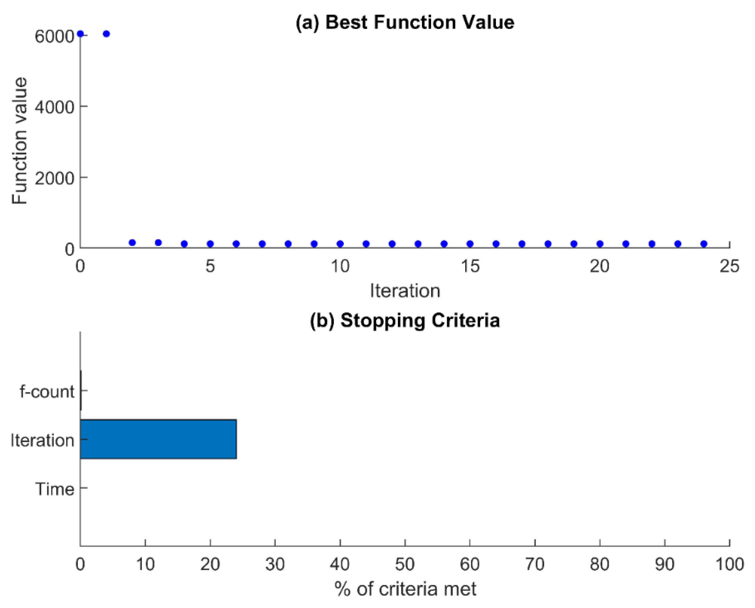
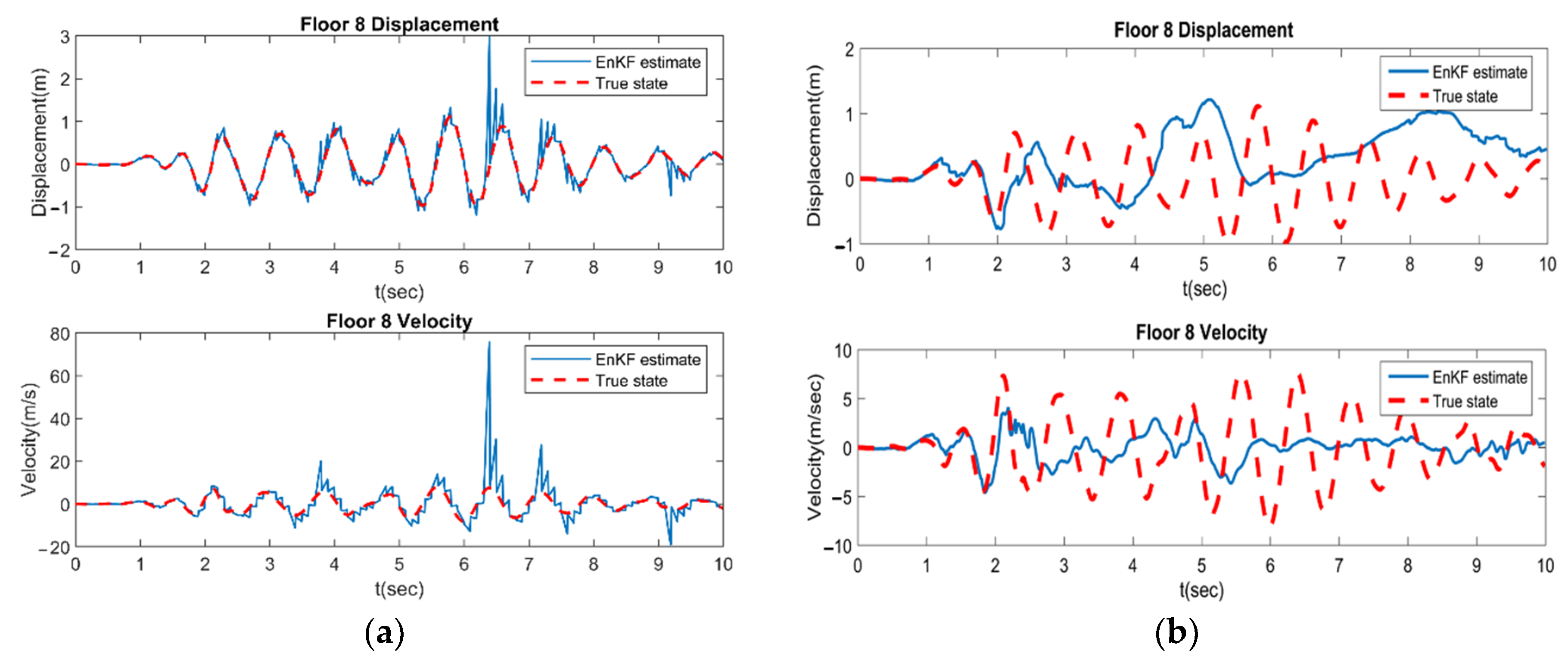
4.1. SA-EnKF Framework

4.1.1. Case 1: Two Available Sensors

When only two sensors are available to be placed on the ten-story building, there are a total of 45 possible sensor location configurations. The algorithm randomly started by placing the two available sensors on floors 4 and 7: initial population {4 7}. The best sensor locations were found to be at floors 3 and 10.

This result is very convincing and logical, since for a limited number of sensors, it is expected that the algorithm must converge to a sensor configuration, where the two sensors can cover the extremities of the building (i.e., one at the top and the second at the bottom) to provide the user with the most instructive measurements.

Figure 2 illustrates the results of the suggested SA-EnKF method for the scenario of two sensors. It is divided into two parts. Figure 2a represents a plot of the best objective function, which is the difference between the actual measured displacements and velocities and the respective predicted values (calculated using Equation (13)) versus the number of iterations of the suggested SA-EnKF approach. As shown in Figure 2a, the fitness value for the initial random population was high, and it started decreasing until it reached a minimum value at the 12th iteration. This value was constant for 20 successive iterations, which made the algorithm stop before reaching the maximum pre-specified number of iterations. This is clearly shown in part Figure 2b, where the algorithm stops before reaching the pre-defined 100 iterations.

It should be noted that the computational burden of the proposed SA-EnKF methodology is relatively acceptable. Figure 3 shows the comparison between the measured and predicted displacement and velocity of floor 8 acquired from the random initial sensor configuration using SA-EnKF framework (Figure 3a) and GA-EnKF methodology (Figure 3b, where the results are taken from [25]). A clear mismatch between the predicted and actual data is noticed when the sensors are randomly placed at the first generation for the two frameworks (note that the scale of the y-axes in parts (a) and (b) is different in Figure 3). Figure 4 represents the comparison between the EnKF predicted values and synthetically measured displacement and velocity of the 8th floor of the building, when the sensors are placed at the optimal locations found using the proposed SA-EnKF approach (Floors 3 and 10) (Figure 4a) and at the GA-EnKF best sensor locations (Floors 1 and 10) (Figure 4b, where the results are taken from [25]).

After analyzing Figure 3a and Figure 4a, a great enhancement was observed in the fitness function, which is the difference between the EnKF estimated displacements and velocities and their respective synthetic exact data when the sensors are placed at the SA-EnKF algorithm’s optimal locations (Floors 3 and 10 for the two). This observation proves the ability of the proposed methodology in converging to some of the best sensor locations, consequently making the process of early damage detection easier.

4.1.2. Case 2: Three Available Sensors

When the available number of sensors for the building under consideration is three, 120 possibilities of sensor location configurations exist. The algorithm randomly started by placing the three available sensors on floors 6, 8 and 10: initial population {6 8 10}. The best sensor locations are found to be at floors 3, 6 and 10. These optimal sensor locations provide a very suitable configuration, where the sensors are placed at the top, middle and bottom ends of the building to provide the user with the most informative measurement data.

Figure 5 illustrates the outcomes of the suggested SA-EnKF methodology for the three sensors case, and it is divided into two parts. Figure 5a represents a plot of the best fitness value, taken as the difference between actual and predicted displacements and velocities, versus the number of iterations of the proposed SA-EnKF methodology. In Figure 5a, the fitness value of the initial population was very high and then decreased to reach a minimum value at the fourth iteration; this value was constant for 20 successive iterations, which forced the algorithm to stop. Figure 5b shows that the algorithm stops before reaching the maximum number of iterations implemented, which is 100 iterations, since the second stopping criterion was satisfied first.

Figure 6 illustrates the difference between the predicted and measured displacement and velocity of floor 8, when sensors are placed on the initial random sensor configurations using the suggested SA-EnKF approach (Figure 6a) and the GA-EnKF framework proposed in [25] (Figure 6b). An obvious discrepancy between the predicted and actual data is present using both methodologies when randomly placing the three sensors at their initial locations. However, the mismatches become negligeable when the sensors were placed at their optimal locations, as found using the SA-EnKF method (Floors 3, 6 and 10) (as shown in Figure 7a) and using the GA-EnKF best sensor locations (Floors 1, 7 and 10) (Figure 7b, where the results are taken from [25]).

After analyzing Figure 6a andFigure 7a, a very good improvement in the difference between the EnKF estimated displacements and velocities and their respective synthetic exact data is clearly shown when the sensors are placed at the SA-EnKF optimal locations (Floors 3, 6 and 10 for the three sensors case). Hence, the SA-EnKF approach converged to some of the optimal sensor locations, consequently helping to make the structural health monitoring and the early damage sensing processes easier.

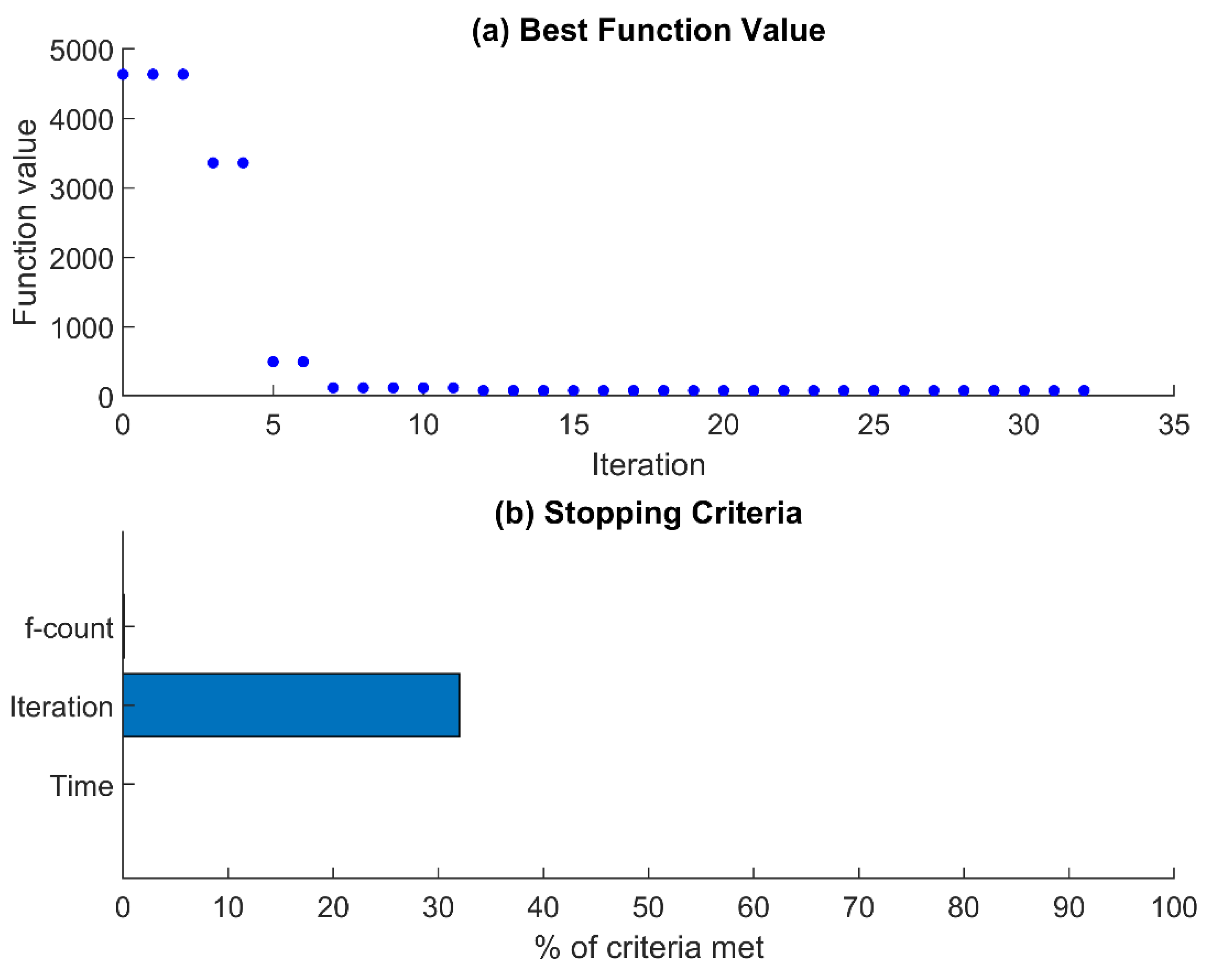
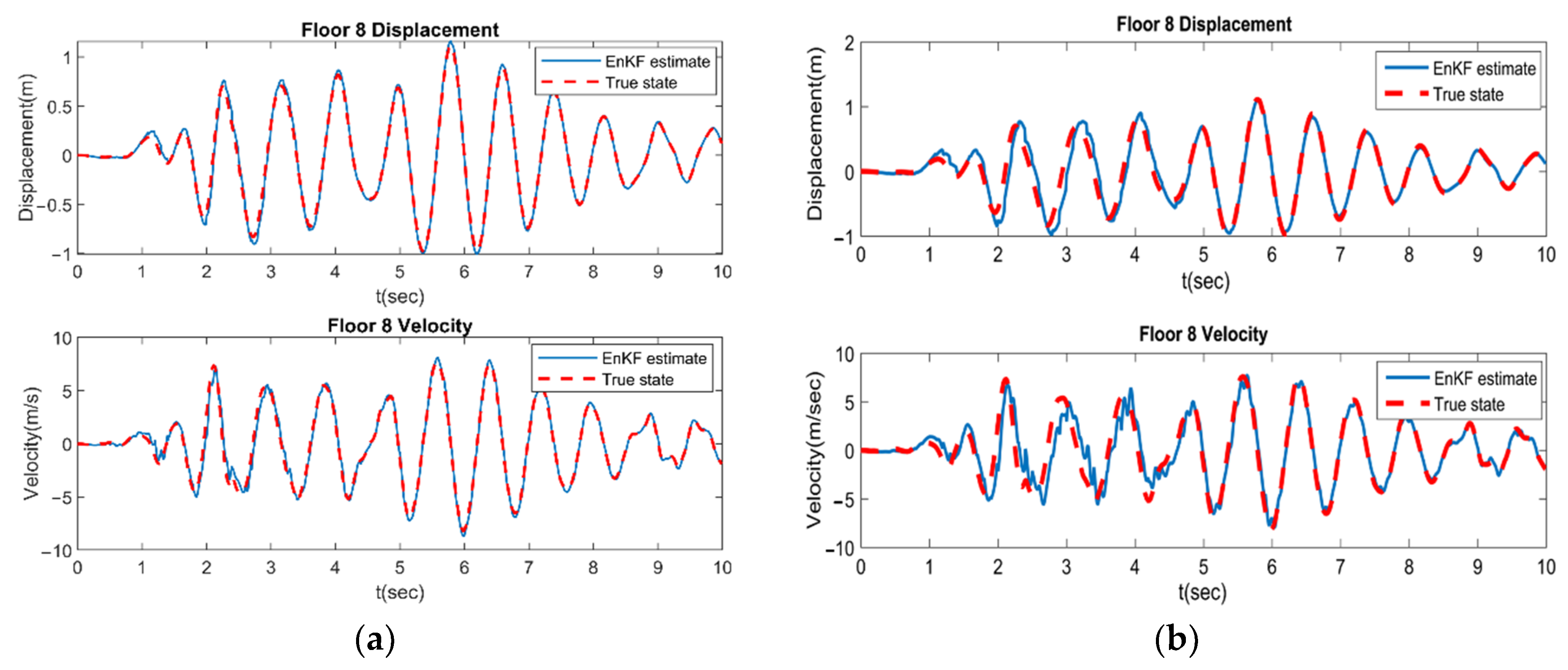
4.2. GA-EnKF Framework

Nasr et al. applied the proposed GA-EnKF framework on the same building considered in this paper. This section presents the corresponding results of this study for comparative purposes [25].

4.2.1. Case 1: Two Available Sensors

For the two sensors scenario, the GA-EnKF algorithm was randomly started by an initial population of sensor locations corresponding to floors 8 and 10: initial population {8 10}. A plateau in the fitness value was achieved after 20 successive iterations, before reaching the maximum number of generations (100), which made the algorithm stop. The best sensor locations were found to be at floors 1 and 10 [25].

4.2.2. Case 2: Three Available Sensors

For the case of the three available sensors, the GA-EnKF algorithm was randomly started by the initial population {2 5 6}, corresponding to placing the sensors on floors 2, 5 and 6. It was shown that the best sensor locations were found to be at floors 1, 7 and 10. For this scenario, the algorithm also stopped before reaching the maximum number of generations, since a negligible difference in the fitness value was recorded for 20 successive generations [25]. It should be noted that while the computational duration for the SA-EnKF methodology to converge to some of the best locations of sensors was around 1.8 × 10³ s, the time taken for the GA-EnKF framework to determine the optimal sensor placements was around 2.5 × 10⁴ s on the same machine. Consequently, the proposed SA-EnKF framework outperforms the GA-EnKF methodology in terms of computational expediency.

4.3. Brute-Force Optimal Results

The brute-force or exhaustive search methodology is implemented in this study to test the accuracy of the proposed SA-EnKF framework in converging to the optimal sensor locations. This general comprehensive search technique consists of analytically computing the fitness function value for each possible scenario of sensor locations.

Table 2. Convergence of SA-EnKF and GA-EnKF to brute-force OSP results.

Number of Sensors	Total Number of Combinations	Brute-Force Approach Optimal Results {Floors}	SA-EnKF Results {Floors}	GA-EnKF Results {Floors}
2	45	{1 10}	{3 10}	{1 10}
3	120	{1 7 10}	{3 6 10}	{1 7 10}

presents the OSP results for the brute-force, the SA-EnKF, and the GA-EnKF [25] methodologies.

For the case of two available sensors, the brute-force search approach evaluates the fitness function value of each possible combination of sensors out of the 45 available scenarios. The lowest mismatch between predicted and measured values, corresponding to the optimal sensor configuration, was found when placing the two sensors on floors 1 and 10, respectively. It was shown that the GA-EnKF results match the brute-force approach optimal results, corresponding to floors 1 and 10 [25]. On the other hand, the SA-EnKF methodology does not converge completely to the optimal brute-force results, but the SA-EnKF optimal configuration is still acceptable for the limited number of available sensors, since the top (floor 10) and the bottom (floor 3) ends of the building are still monitored in this case.

For the case of three available sensors, after computing the penalty value of each combination of the 120 available scenarios, the brute-force search approach showed that the lowest mismatch between predicted and actual data, corresponding to the best configuration, is reached when placing the three sensors on floors 1, 7 and 10. The GA-EnKF results converged to the brute-force optimal results, corresponding to placing the three sensors on floors 1, 7 and 10, proving the robustness of this methodology [25]. In contrast, although the SA-EnKF results do not match the optimal results of the brute-force approach they are still satisfactory since the top (floor 10), the middle (floor 6), and the bottom (floor 3) ends of the building are also instrumented in this case.

Figure 8 represents a summary of the numerical example results, showing a comparison between the GA-EnKF and the SA-EnKF outcomes for the two scenarios of the available number of sensors. This figure also explicitly shows the optimal sensor configurations found using both methodologies for the two cases of available sensors. For the two sensors case (blue line), it is clearly shown that the GA-EnKF approach converges to a better solution of sensor locations (GA-EnKF best sensor locations: floors 1 and 10) than that of the SA-EnKF method (SA-EnKF optimal sensor locations: floors 3 and 10). This is represented through the values of the penalty function, which is the mismatch between actual and predicted displacement and velocity of the various stories of the building at the corresponding optimal sensor configurations. While the penalty value related to the best sensor locations (placing the two sensors at floors 1 and 10) is equal to 258.87 for the GA-EnKF approach, the fitness function value related to the optimal sensor configuration (placing the two sensors at floors 3 ad 10) is found to be 291.59 for the SA-EnKF case. On the other hand, the SA-EnKF methodology requires less computational time than the GA-EnKF approach. For the three sensors case (red line), Figure 8 shows that although the GA-EnKF method converged to better sensor locations (penalty value equals 142.31 when placing the sensors at their optimal locations on floors 1, 7 and 10) than the SA-EnKF method, the optimal sensor locations found using the SA-EnKF framework (floors 3, 6 and 10) are considered very acceptable (penalty value equals 227.68), especially since this algorithm requires much less computational burden than the GA-EnKF methodology.

Thus, although the proposed SA-EnKF framework did not totally converge to the optimal results of the brute-force method, for both cases of the available number of sensors, it succeeded in determining some very suitable locations for the placement of sensors. This was clearly demonstrated through the acceptable low values of the penalty functions associated with placing the available sensors at the best locations of SA-EnKF. This was also clearly shown in Figure 3 and Figure 4, for the two sensors scenario, and in Figure 6 and Figure 7 for the three sensors case, where a very good improvement in the mismatch between the EnKF predictions and the synthetic measured values of the displacement and velocity, was detected when the sensors were placed at the SA-EnKF optimal locations. Furthermore, although the GA-EnKF method outperformed the proposed SA-EnKF in terms of accuracy of the results in converging to the best sensor locations, the SA-EnKF showed a much better performance than the other framework in terms of computational effort and expenses.

5. Conclusions

In this study, a robust optimal sensor placement approach, which comprises a combination between an optimization-based algorithm, the simulated annealing method, and the ensemble Kalman filter technique, is presented for structural health monitoring and early damage sensing purposes.

The suggested SA-EnKF framework enhances the suitability and robustness of the optimization-based algorithms to solve a broad variety of problems with nonlinear and hysteretic behaviors and with a limited amount of real-time online monitoring data. It is shown that even for a limited number of available sensors, the EnKF technique is effectively capable of estimating and correcting the system state and unknown model parameters, every time measurement data are available. On the other hand, the SA algorithm successfully minimizes the corresponding objective function and consequently determines some of the best locations of the available number of sensors.

The optimal locations of two and three available sensors are determined on a ten-story building subjected to El Centro earthquake excitation at its base using the proposed SA-EnKF approach. The SA algorithm randomly generates an initial population of sensor locations. The objective function for the SA algorithm is determined by minimizing the difference between the synthetic actual measured displacements and velocities of the different floors of the building and their corresponding predicted values, estimated using the EnKF technique. It is shown that placing the sensors at their SA-EnKF optimal locations on the structure, decreases the mismatch between the synthetic real measured data and their corresponding EnKF estimated values, consequently validating the effectiveness of the proposed algorithm.

A comparative analysis between two optimization-based frameworks, primarily the GA-EnKF and the SA-EnKF methodologies, is performed. Both algorithms are tested on the same building subjected to the same earthquake excitation exerted at its base. The comparison is based on computational burden and the accuracy of each methodology converging to the best sensor locations.

The validity and accuracy of the GA-EnKF and the SA-EnKF results are tested through a comparison with the optimal sensor locations of the brute-force search methodology, which comprises a systematic computation of the fitness function of each possible sensor configuration for the two cases of available sensors. For the case of two available sensors, the optimal locations are found to be on floors {3 10} using the SA-EnKF algorithm and on floor {1 10} using the GA-EnKF framework. The brute-force approach optimal results are achieved when placing the two sensors on floors 1 and 10. For the three available sensors case, the best locations are found to be on floors {3 6 10} using the proposed SA-EnKF approach and on floors {1 7 10} using the GA-EnKF methodology. The optimal sensor locations detected using the brute-force approach are on floors 1, 7 and 10.

The SA-EnKF algorithm can be effectively used to determine the limited number of monitoring devices necessary to cover a whole instrumented structure. The accuracy of the GA-EnKF approach outperforms the SA-EnKF in terms of converging to the optimal brute-force results but at significantly higher computational costs. A trade-off between the outcome precision and complexity of computation must be considered in order to select the optimized-based framework for structural health monitoring and damage detection purposes.

References

1. Guo, H.Y.; Zhang, L.; Zhang, L.L.; Zhou, J.X. Optimal placement of sensors for structural health monitoring using improved genetic algorithms. Smart Mater. Struct. 2004, 13, 528. [Google Scholar] [CrossRef]
2. Nasr, D.; Slika, W.; Saad, G. Uncertainty Quantification for Structural Health Monitoring Applications. Smart Struct. Syst. 2018, 22, 399–411. [Google Scholar]
3. Sebt, M.H.; Yousefzadeh, A.; Tehranizadeh, M. The optimal TADAS damper placement in moment resisting steel structures based on a cost-benefit analysis. Int. J. Civ. Eng. 2011, 9, 23–32. [Google Scholar]
4. Abbasi, M.; Davaei-Markazi, A.H. Optimal assignment of seismic vibration control actuators using genetic algorithm. Int. J. Civ. Eng. 2014, 12, 24–31. [Google Scholar]
5. Downey, A.; Hu, C.; Laflamme, S. Optimal sensor placement within a hybrid dense sensor network using an adaptive genetic algorithm with learning gene pool. Struct. Health Monit. 2018, 17, 450–460. [Google Scholar] [CrossRef]
6. Hou, R.; Xia, Y.; Xia, Q.; Zhou, X. Genetic algorithm based optimal sensor placement for L1-regularized damage detection. Struct. Control Health Monit. 2019, 26, e2274. [Google Scholar] [CrossRef]
7. Su, J.B.; Luan, S.L.; Zhang, L.M.; Zhu, R.H.; Qin, W.G. Partitioned genetic algorithm strategy for optimal sensor placement based on structure features of a high-piled wharf. Struct. Control Health Monit. 2019, 26, e2289. [Google Scholar] [CrossRef]
8. Papadimitriou, C.; Beck, J.L.; Au, S.K. Entropy-based optimal sensor location for structural model updating. J. Vib. Control 2000, 6, 781–800. [Google Scholar] [CrossRef]
9. Flynn, E.B.; Todd, M.D. A Bayesian approach to optimal sensor placement for structural health monitoring with application to active sensing. Mech. Syst. Signal Process. 2010, 24, 891–903. [Google Scholar] [CrossRef]
10. Chow, H.; Lam, H.F.; Yin, T.; Au, S.K. Optimal sensor configuration of a typical transmission tower for the purpose of structural model updating. Struct. Control Health Monit. 2011, 18, 305–320. [Google Scholar] [CrossRef]
11. Ponticelli, G.S.; Guarino, S.; Giannini, O. An optimal genetic algorithm for fatigue life control of medium carbon steel in laser hardening process. Appl. Sci. 2020, 10, 1401. [Google Scholar] [CrossRef]
12. Assaad, J.; Nasr, D.; Chwaifaty, S.; Tawk, T. Parametric study on polymer-modified pigmented cementitious overlays for colored applications. J. Build Eng. 2020, 27, 101009. [Google Scholar] [CrossRef]
13. Assaad, J.; Nasr, D.; Gerges, N.; Issa, C. Use of soft computing techniques to predict the bond to reinforcing bars of underwater concrete. Int. J. Civ. Eng. 2021, 19, 669–683. [Google Scholar] [CrossRef]
14. Chiu, P.L.; Lin, F.Y. A simulated annealing algorithm to support the sensor placement for target location. In Proceedings of the Canadian Conference on Electrical and Computer Engineering, Niagara Falls, OT, Canada, 2–5 May 2004. [Google Scholar]
15. Lin, F.Y.; Chiu, P. A near-optimal sensor placement algorithm to achieve complete coverage-discrimination in sensor networks. IEEE Commun. Lett. 2005, 9, 43–45. [Google Scholar]
16. Tong, K.H.; Bakhary, N.; Kueh, A.B.H.; Yassin, A.Y. Optimal sensor placement for mode shapes using improved simulated annealing. Smart Struct. Syst. 2014, 13, 389–406. [Google Scholar] [CrossRef]
17. Leitold, D.; Vathy-Fogarassy, A.; Abonyi, J. Network distance-based simulated annealing and fuzzy clustering for sensor placement ensuring observability and minimal relative degree. Sensors 2018, 18, 3096. [Google Scholar] [CrossRef]
18. Augugliaro, A.; Dusonchet, L.; Sanseverino, E.R. Genetic, simulated annealing and tabu search algorithms: Three heuristic methods for optimal reconfiguration and compensation of distribution networks. Eur. Trans. Electr. Power 1999, 9, 35–41. [Google Scholar] [CrossRef]
19. Hasan, M.; AlKhamis, T.; Ali, J. A comparison between simulated annealing, genetic algorithm and tabu search methods for the unconstrained quadratic Pseudo-Boolean function. Comput. Ind. Eng. 2000, 38, 323–340. [Google Scholar] [CrossRef]
20. Arostegui, M.A.; Kadipasaoglu, S.N.; Khumawala, B.M. An empirical comparison of tabu search, simulated annealing, and genetic algorithms for facilities location problems. Int. J. Prod. Econ. 2006, 103, 742–754. [Google Scholar] [CrossRef]
21. Garlapati, V.K.; Vundavilli, P.R.; Banerjee, R. Evaluation of lipase production by genetic algorithm and particle swarm optimization and their comparative study. Appl. Biochem. Biotechnol. 2010, 162, 1350–1361. [Google Scholar] [CrossRef]
22. Kahouli, O.; Alsaif, H.; Bouteraa, Y.; Ben Ali, N.; Chaabene, M. Power System Reconfiguration in Distribution Network for Improving Reliability Using Genetic Algorithm and Particle Swarm Optimization. Appl. Sci. 2021, 11, 3092. [Google Scholar] [CrossRef]
23. Evensen, G. Sequential data assimilation with a nonlinear quasi-geostrophic model using Monte Carlo to forecast error statistics. J. Geophys. Res. Oceans 1994, 99, 10143–10162. [Google Scholar] [CrossRef]
24. Nasr, D.E.; Saad, G.A. Sensor placement optimization using Ensemble Kalman Filter and Genetic Algorithm. In Proceedings of the 5th International Conference on Computational Methods in Structural Dynamics and Earthquake Engineering (COMPDYN 2015), Crete, Greece, 25–27 May 2015. [Google Scholar]
25. Nasr, D.E.; Saad, G.A. Optimal Sensor Placement Using a Combined Genetic Algorithm–Ensemble Kalman Filter Framework. ASCE ASME J. Risk Uncertain Eng. Syst. A Civ. Eng. 2016, 3, 04016010. [Google Scholar] [CrossRef]
26. Holland, J.H. Adaptation in Natural and Artificial Systems: An Introductory Analysis with Applications to Biology, Control, and Artificial Intelligence; U Michigan Press: Oxford, UK, 1975. [Google Scholar]
27. Chou, J.H.; Ghabboussi, J. Genetic algorithm in structural damage detection. Comput. Struct. 2001, 79, 1335–1353. [Google Scholar] [CrossRef]
28. Kirkpatrick, S.; Vecchi, M.P. Optimization by simulated annealing. Science 1983, 220, 671–680. [Google Scholar] [CrossRef] [PubMed]
29. Jacobson, L. Simulated Annealing for Beginners. 2013. Available online: http://www.theprojectspot.com/tutorial-post/simulated-annealing-algorithm-for-beginners/6 (accessed on 27 July 2020).
30. Kalman, R.E. A new approach to linear filtering and prediction problems. J. Basic Eng. 1960, 82, 35–45. [Google Scholar] [CrossRef]
31. Burgers, G.; Leeuwen, P.; Evensen, G. Analysis scheme in the ensemble Kalman filter. Mon. Weather Rev. 1998, 126, 1719–1724. [Google Scholar] [CrossRef]
32. Welch, G.; Bishop, G. An Introduction to the Kalman Filter; University of North Carolina: Chapel Hill, NC, USA, 2006. [Google Scholar]
33. Grewal, M.; Andrews, A. Kalman Filtering Theory and Applications Using MATLAB, 3rd ed.; John Wiley & Sons: Hoboken, NJ, USA, 2008. [Google Scholar]
34. Chatzi, E.N.; Smyth, A.W. The unscented Kalman filter and particle filter methods for nonlinear structural system identification with non-collocated heterogeneous sensing. Struct. Control Health Monit. 2009, 16, 99–123. [Google Scholar] [CrossRef]
35. Ghanem, R.; Ferro, G. Health monitoring of strongly nonlinear systems using the ensemble Kalman filter. Struct. Control Health Monit. 2006, 13, 245–259. [Google Scholar] [CrossRef]
36. Saad, G.; Ghanem, R.; Masri, S. Robust system identification of strongly non-linear dynamics using a polynomial chaos based sequential data assimilation technique. In Proceedings of the 48th AIAA/ASME/ASCE/AHS/ASC Structures, Structural Dynamics and Materials Conference, Honolulu, HI, USA, 23–27 April 2007. [Google Scholar]
37. Saad, G.; Ghanem, R. Robust Structural Health Monitoring using a polynomial chaos sequential data assimilation technique. In Proceedings of the 3rd International Conference on Computational Methods in Structural Dynamics and Earthquake Engineering (COMPDYN 2011), Corfu, Greece, 26–28 May 2011. [Google Scholar]
Figure 1. The general outline of the SA-EnKF framework.
Buildings 12 01383 g001
Figure 2. Two-sensors case: (a) Dots representing the best fitness value at every iteration and (b) stopping criteria.
Buildings 12 01383 g002
Figure 3. Two-sensors case: Estimates of the 8th floor displacement and velocity at initial sensor locations: (a) using SA-EnKF and (b) using GA-EnKF (results taken from [25]).
Buildings 12 01383 g003
Figure 4. Two-sensors case: Estimates of the 8th floor displacement and velocity at final iteration: (a) at SA-EnKF Optimal sensor locations (Floors 3 and 10) and (b) at GA-EnKF Optimal Sensor Locations (Floors 1 and 10) (Results taken from [25]).
Buildings 12 01383 g004
Figure 5. Three-sensors case: (a) Dots representing the best fitness value at every iteration and (b) stopping criteria.
Buildings 12 01383 g005
Figure 6. Three-sensors case: Estimates of the 8th floor displacement and velocity at initial sensor locations: (a) using SA-EnKF and (b) using GA-EnKF (results taken from [25]).
Buildings 12 01383 g006
Figure 7. Three-sensors case: Estimates of the 8th floor displacement and velocity at final iteration: (a) at SA-EnKF optimal sensor locations (Floors 3, 6 and 10) and (b) at GA-EnKF optimal sensor locations (Floors 1, 7 and 10) (results taken from [25]).
Buildings 12 01383 g007
Figure 8. GA-EnKF and SA-EnKF penalty values corresponding to the optimal sensor locations versus computational time.
Buildings 12 01383 g008