
A Simple Calibrated Ductile Fracture Model and Its Application in Failure Analysis of Steel Connections

Abstract
:1. Introduction
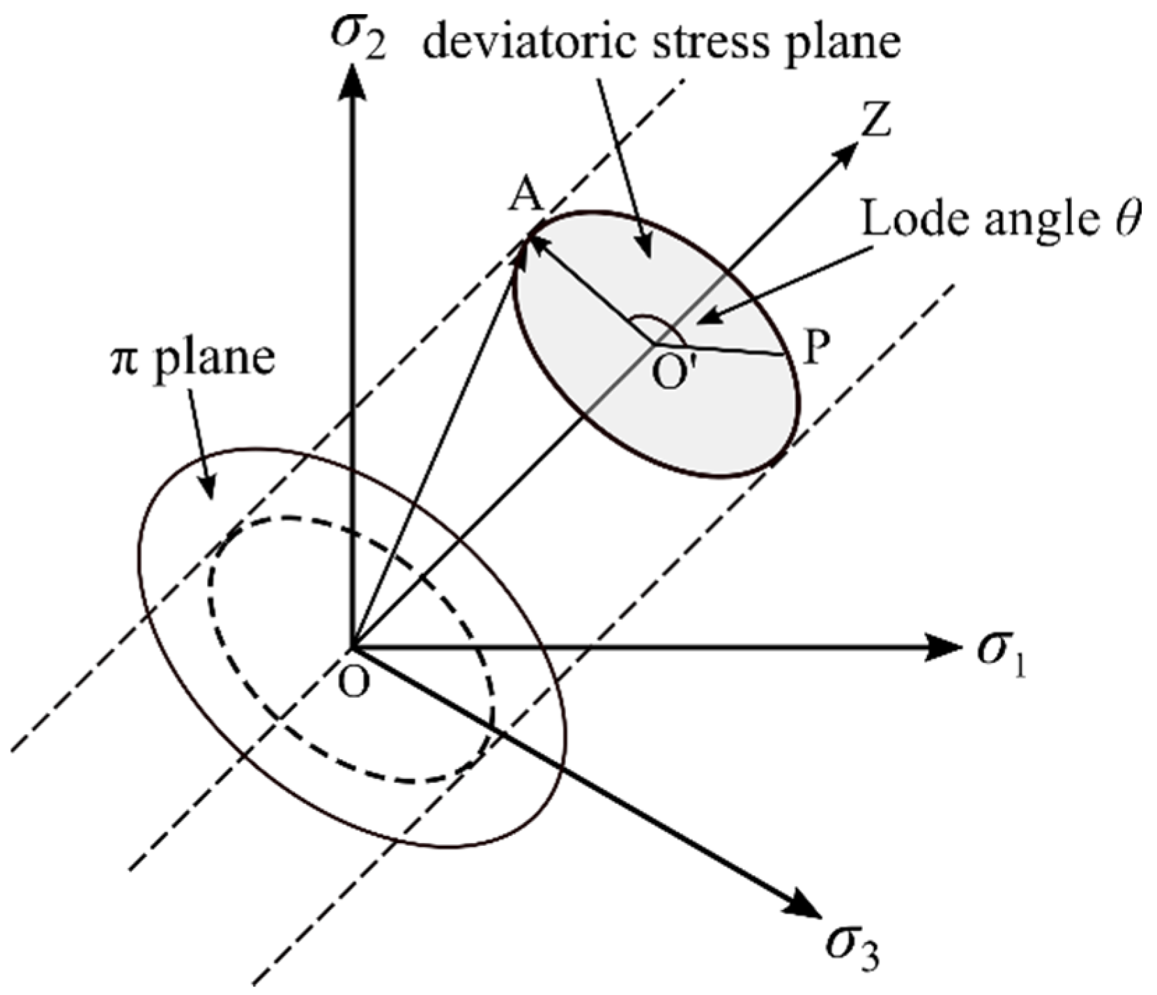
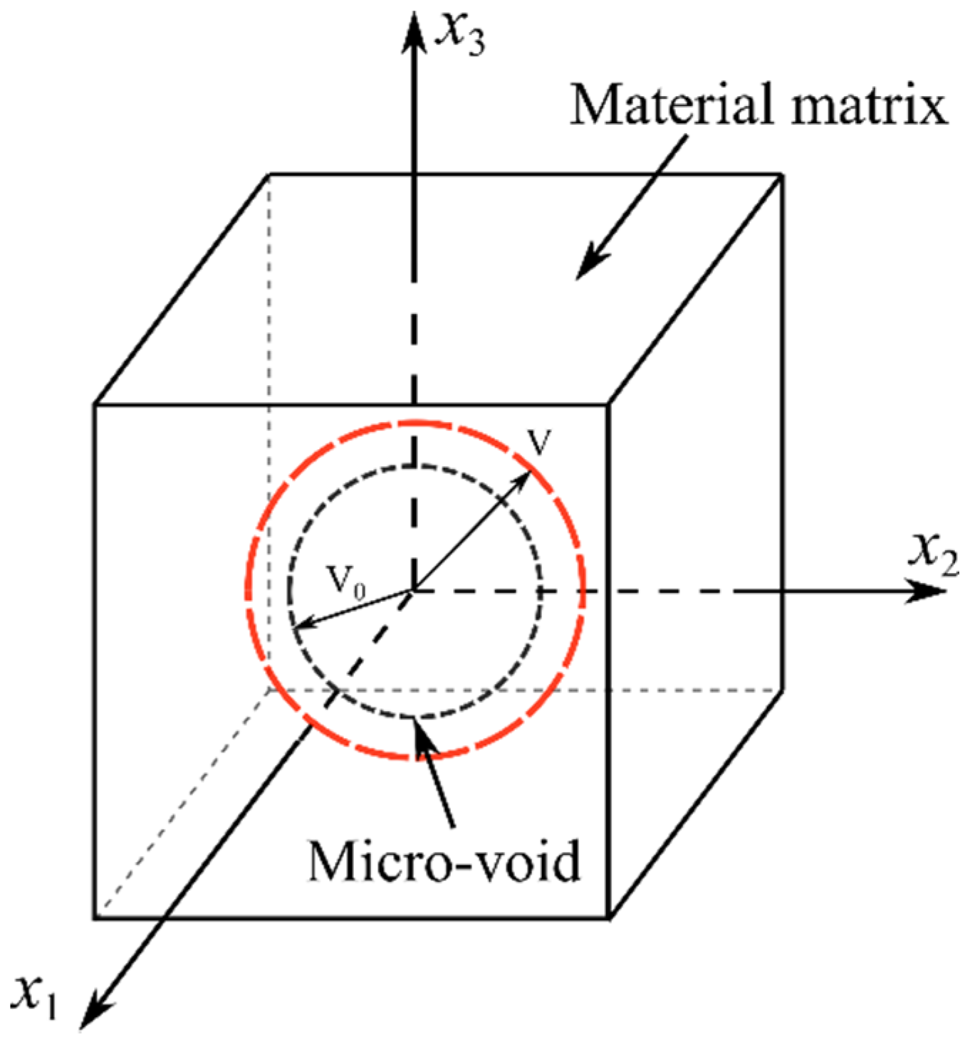
2. Characterization of Material’s Ductility and Stress State
3. Theoretical Derivation of the New Ductile Fracture Model
3.1. Determination of Stress Triaxiality Dependence Function
3.2. Determination of the Lode Angle Dependence Function
3.3. Theoretical Formula of the New Fracture Model
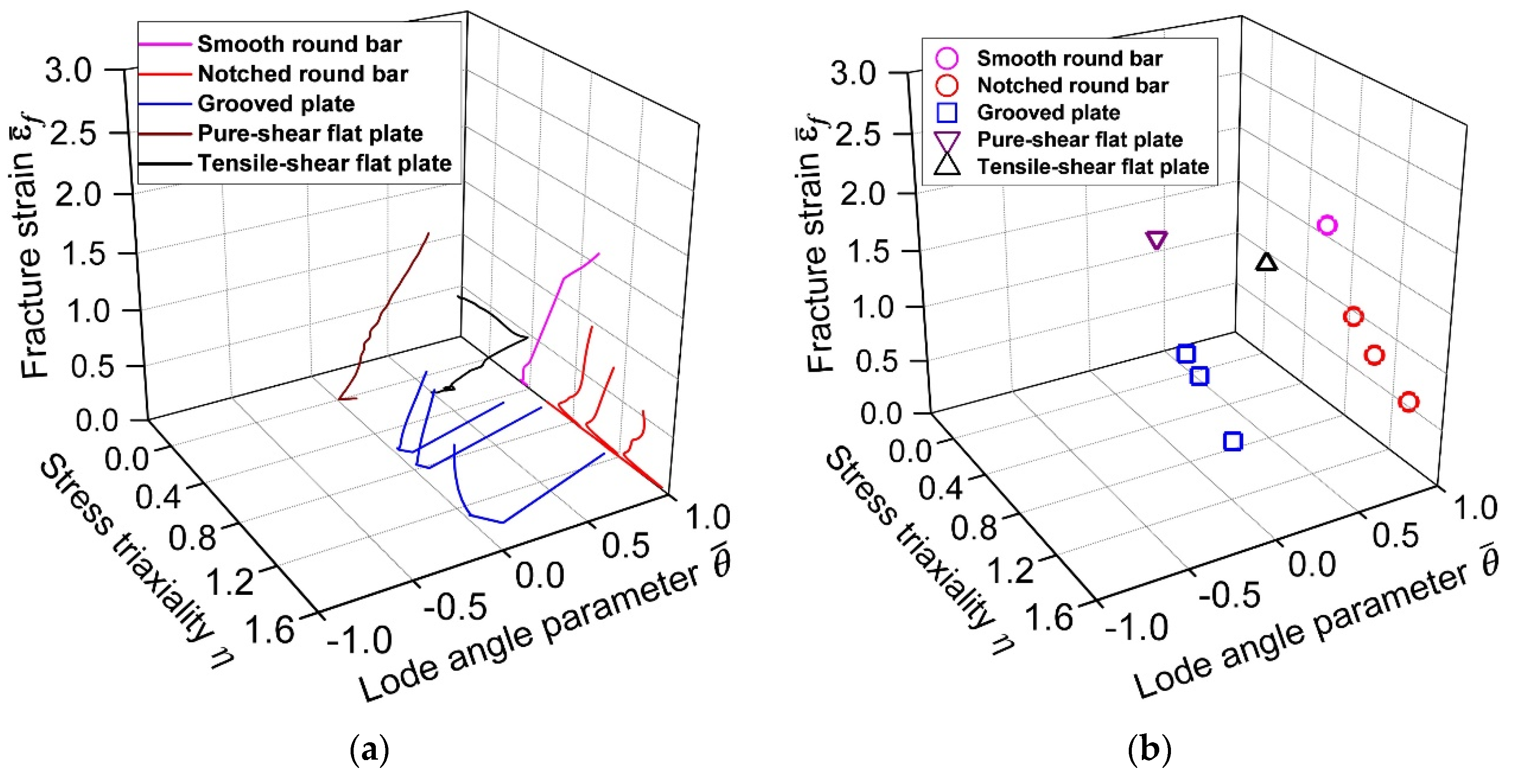
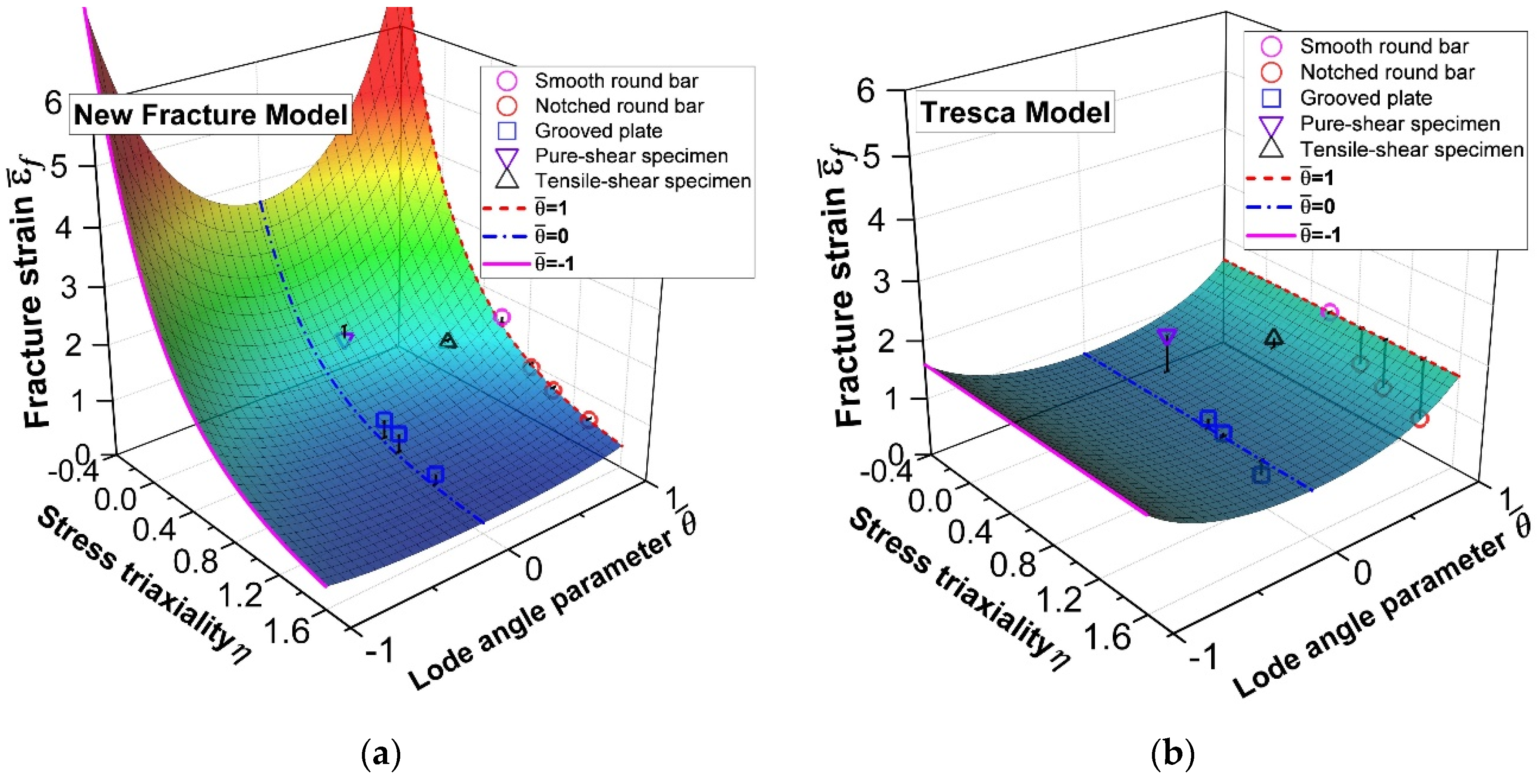
4. Verification of the New Fracture Model via Structural Steel Notched Specimens
5. Application of New Fracture Model in Failure Analysis of Steel Connections
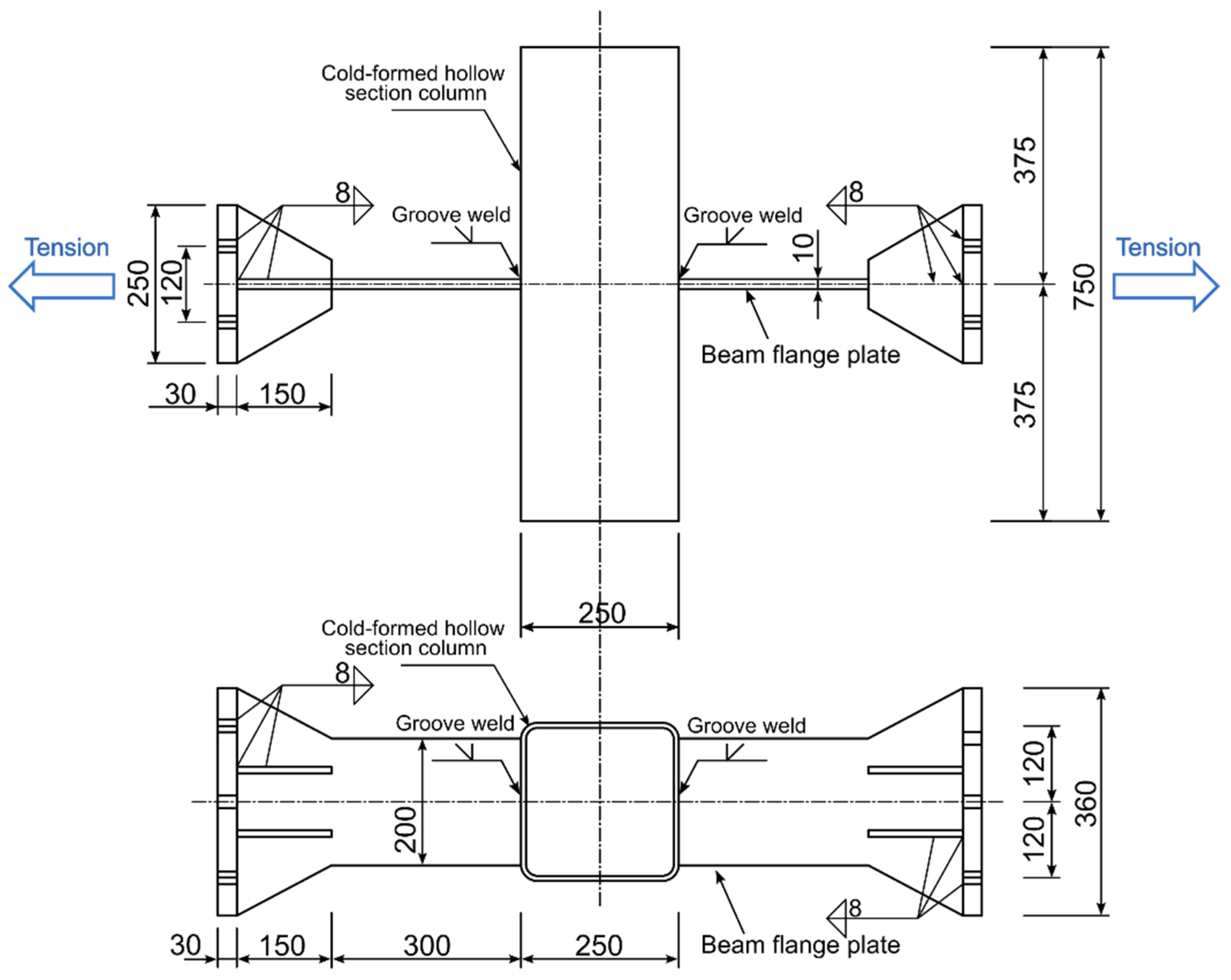
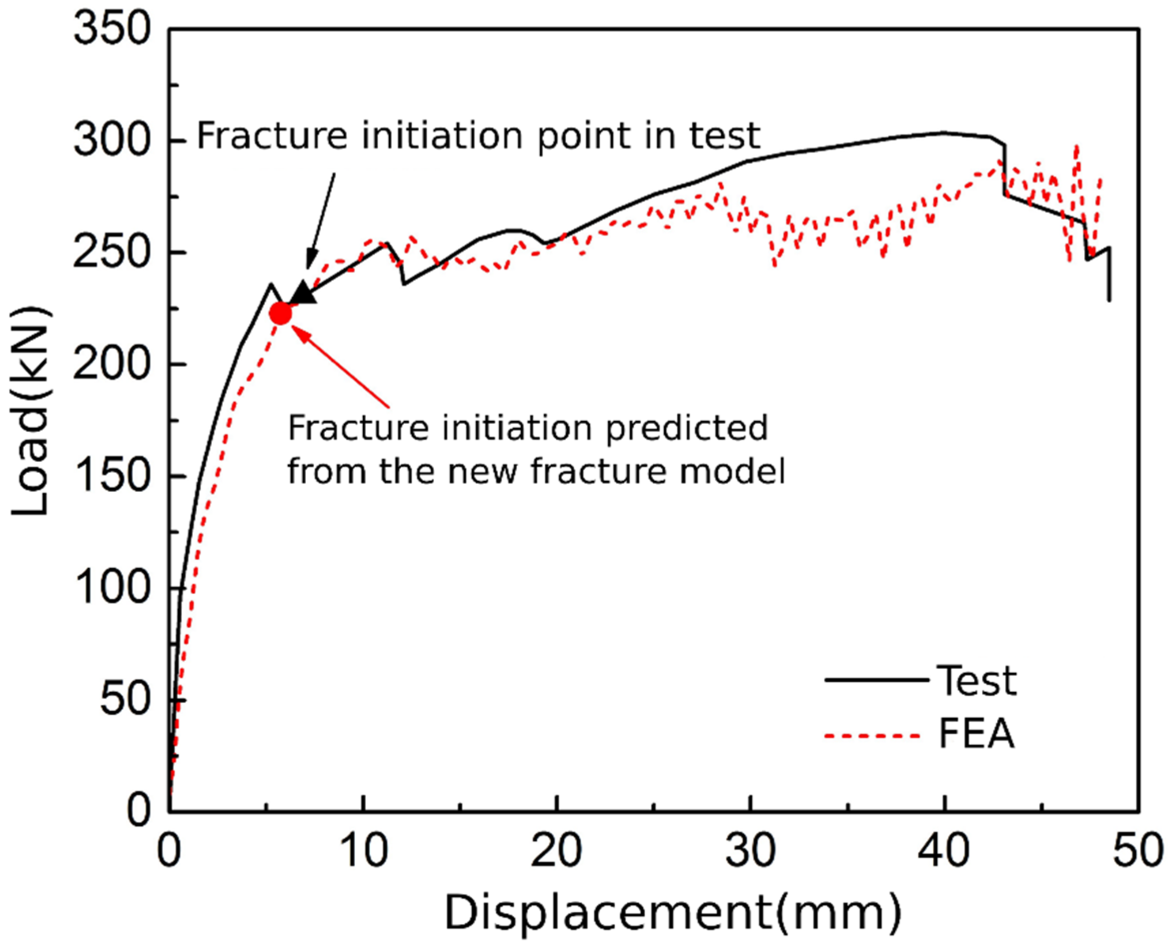
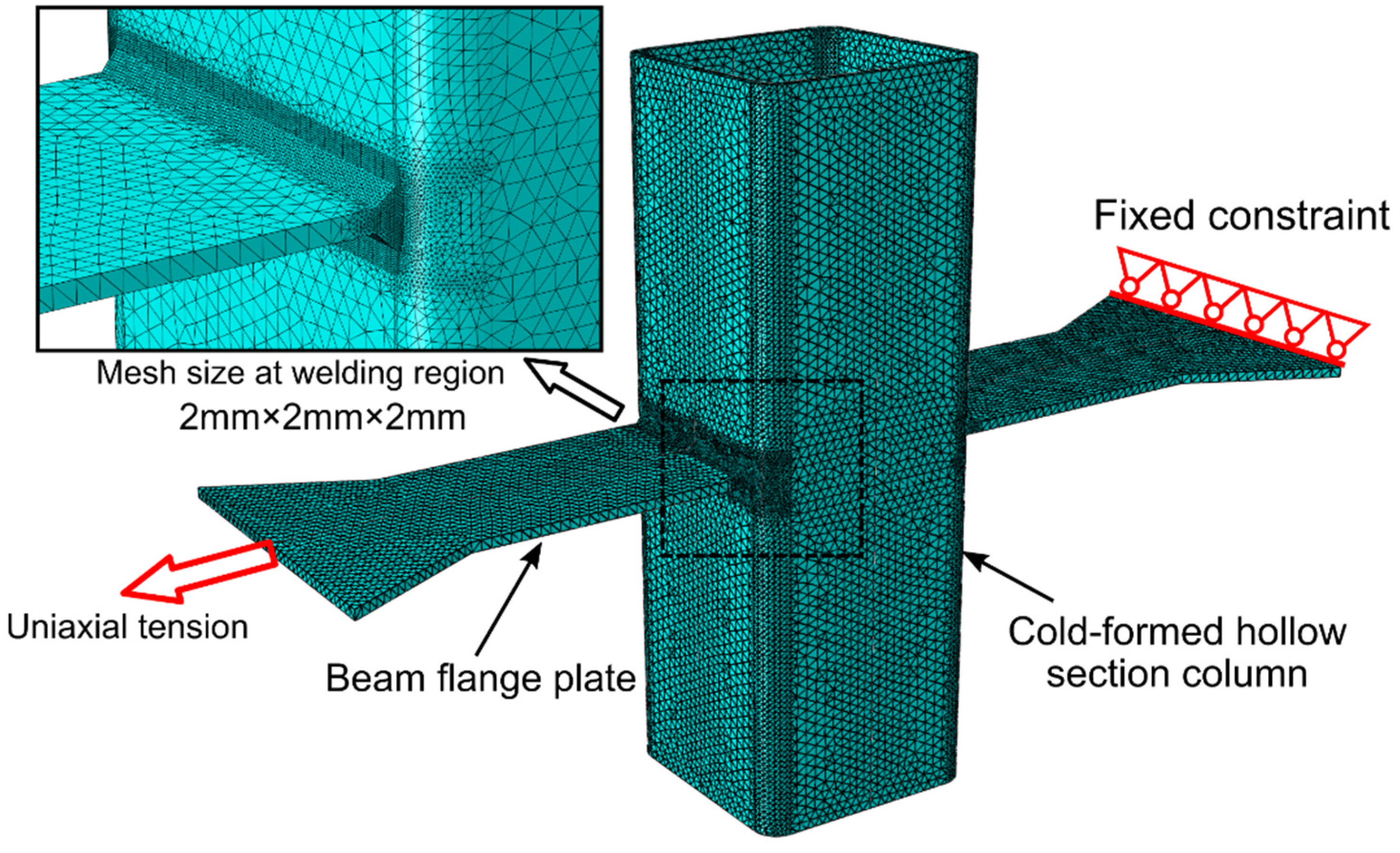
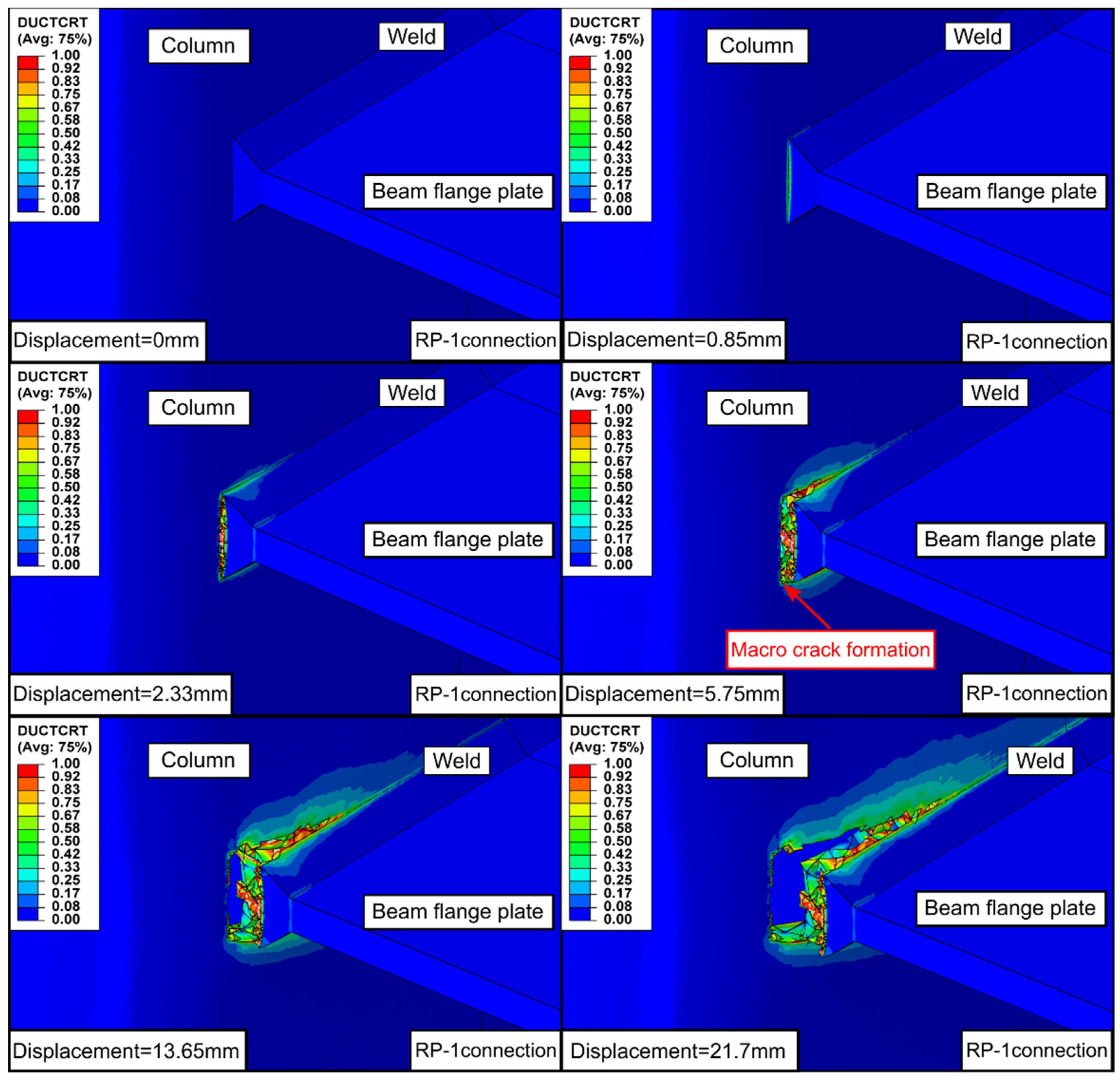
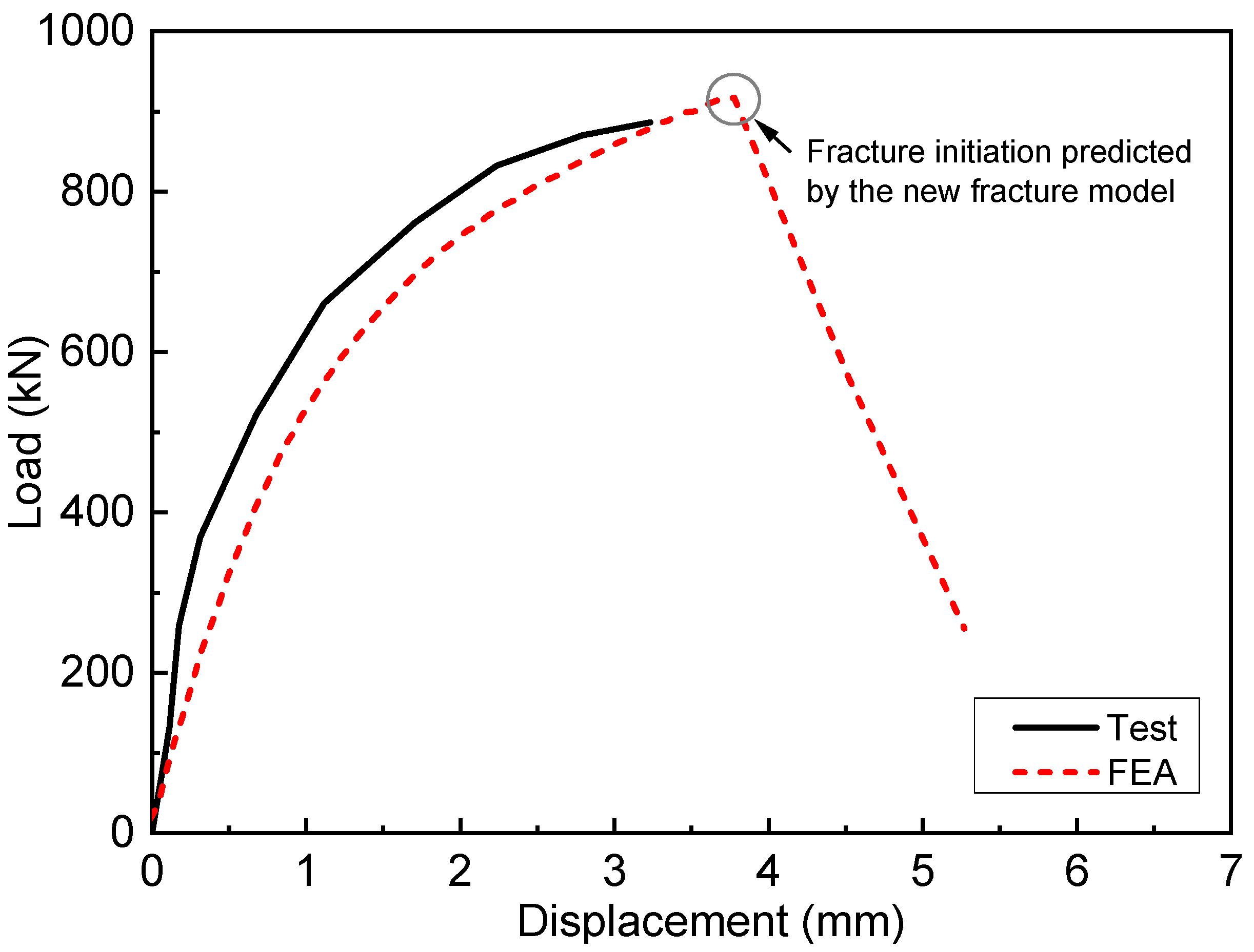
5.1. Fracture Prediction Analysis of a Welded Beam-To-Column Connection
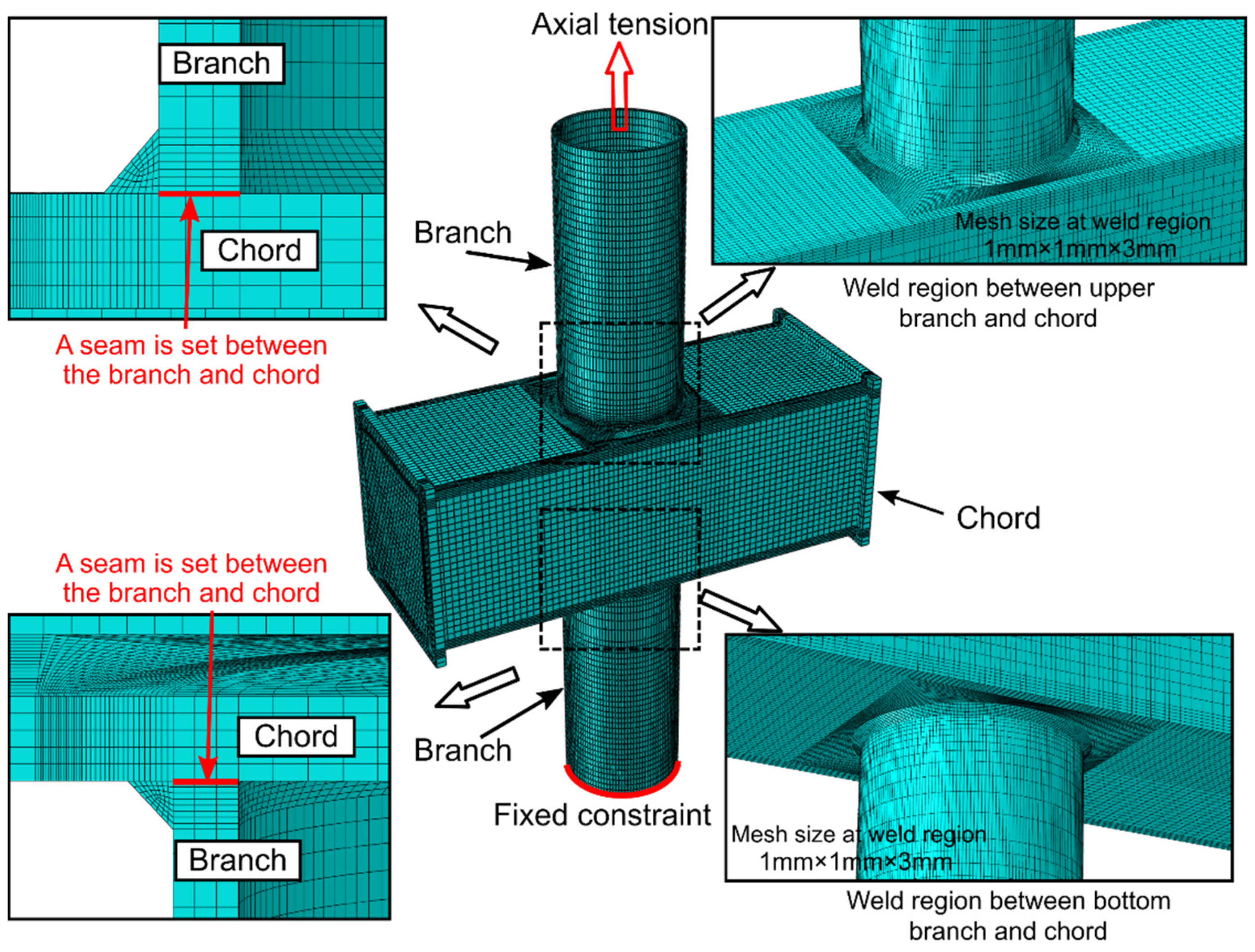
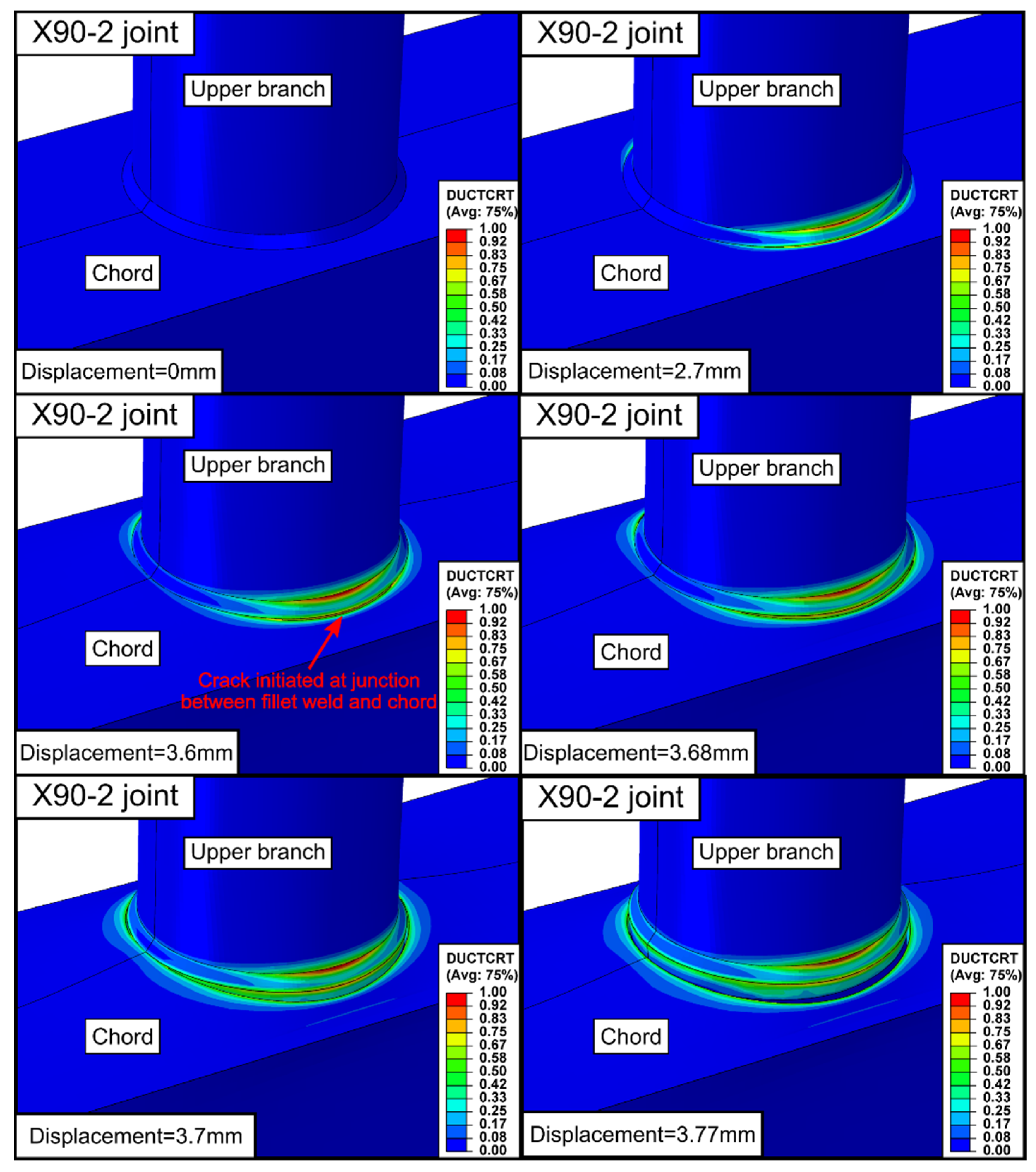
5.2. Fracture Prediction Analysis of a CHS Branch to SHS Chord X-Joint
6. Discussion
6.1. The Correlation between Stress Triaxiality and Lode Angle Dependence
6.2. Validity of Stress Triaxiality Dependence Function for Other Stress States
6.3. Methods to Improve the Prediction Accuracy of the Proposed Fracture Model
7. Conclusions
Author Contributions
Funding
Institutional Review Board Statement
Informed Consent Statement
Data Availability Statement
Conflicts of Interest
References
- Kuwamura, H. Fracture of steel during an earthquake—State-of-the-art in Japan. Eng. Struct. 1998, 20, 310–322. [Google Scholar] [CrossRef]
- Okazaki, T.; Lignos, D.G.; Midorikawa, M.; Ricles, J.; Love, J. Damage to steel buildings observed after the 2011 Tohoku-Oki earthquake. Earthq. Spectra 2013, 29, 219–243. [Google Scholar] [CrossRef]
- Okazaki, T.; Arce, G.; Ryu, H.; Engelhardt, M. Experimental study of local buckling, overstrength, and fracture of links in eccentrically braced frames. J. Struct. Eng. 2005, 131, 1526–1535. [Google Scholar] [CrossRef]
- Chao, S.; Khandelwal, K.; El-Tawil, S. Ductile web fracture initiation in steel shear links. J. Struct. Eng. 2006, 132, 1192–1200. [Google Scholar] [CrossRef]
- Achouri, M.; Germain, G.; Dal, P.; Saidane, D. Experimental characterization and numerical modeling of micromechanical damage under different stress states. Mater. Des. 2013, 50, 207–222. [Google Scholar] [CrossRef]
- Mohr, D.; Marcadet, S. Micromechanically-motivated phenomenological Hosford–Coulomb model for predicting ductile fracture initiation at low stress triaxialities. Int. J. Solids Struct. 2015, 67–68, 40–55. [Google Scholar] [CrossRef]
- Brünig, M.; Gerke, S.; Hagenbrock, V. Micro-mechanical analyses of the effect of stress triaxiality and the Lode parameter on ductile damage and failure. Int. J. Plast. 2013, 50, 49–65. [Google Scholar] [CrossRef]
- Dunand, M.; Mohr, D. Effect of Lode parameter on plastic flow localization after proportional loading at low stress triaxialities. J. Mech. Phys. Solids 2014, 66, 133–153. [Google Scholar] [CrossRef]
- Lou, Y.; Yoon, J.; Huh, H.; Chao, Q.; Song, J. Correlation of the maximum shear stress with micro-mechanisms of ductile fracture for metals with high strength-to-weight ratio. Int. J. Mech. Sci. 2018, 146–147, 583–601. [Google Scholar] [CrossRef]
- Keralavarma, S.; Reddi, D.; Benzerga, A. Ductile failure as a constitutive instability in porous plastic solids. J. Mech. Phys. Solids 2020, 139, 103917. [Google Scholar] [CrossRef]
- Lee, B.; Mear, M. Axisymmetric deformation of power-law solids containing a dilute concentration of aligned spheroidal voids. J. Mech. Phys. Solids 1992, 40, 1805–1836. [Google Scholar] [CrossRef]
- Bao, Y.; Wierzbicki, T. On fracture locus in the equivalent strain and stress triaxiality space. Int. J. Mech. Sci. 2004, 46, 81–98. [Google Scholar] [CrossRef]
- Bai, Y.; Wierzbicki, T. Application of extended Mohr–Coulomb criterion to ductile fracture. Int. J. Fract. 2009, 161, 1. [Google Scholar] [CrossRef]
- Khan, A.; Liu, H. A new approach for ductile fracture prediction on Al 2024-T351 alloy. Int. J. Plast. 2012, 35, 1–12. [Google Scholar] [CrossRef]
- Lou, Y.; Yoon, J.; Huh, H. Modeling of shear ductile fracture considering a changeable cut-off value for stress triaxiality. Int. J. Plast. 2014, 54, 56–80. [Google Scholar] [CrossRef]
- Lou, Y.; Chen, L.; Clausmeyer, T.; Tekkaya, A.; Yoon, J. Modeling of ductile fracture from shear to balanced biaxial tension for sheet metals. Int. J. Solids Struct. 2017, 112, 169–184. [Google Scholar] [CrossRef]
- Roth, C.; Mohr, D. Ductile fracture experiments with locally proportional loading histories. Int. J. Plast. 2016, 79, 328–354. [Google Scholar] [CrossRef]
- Brünig, M.; Gerke, S.; Schmidt, M. Damage and failure at negative stress triaxialities: Experiments, modeling and numerical simulations. Int. J. Plast. 2018, 102, 70–82. [Google Scholar] [CrossRef]
- Gurson, A. Continuum theory of ductile rupture by void nucleation and growth: Part I—yield criteria and flow rules for porous ductile media. J. Eng. Mater. Technol. 1977, 99, 2–15. [Google Scholar] [CrossRef]
- Tvergaard, V.; Needleman, A. Analysis of the cup-cone fracture in a round tensile bar. Acta Metall. 1984, 32, 157–169. [Google Scholar] [CrossRef]
- Lemaitre, J. A continuous damage mechanics model for ductile fracture. J. Eng. Mater. Technol. 1985, 107, 83–89. [Google Scholar] [CrossRef]
- Wierzbicki, T.; Bao, Y.; Lee, Y.; Bai, Y. Calibration and evaluation of seven fracture models. Int. J. Mech. Sci. 2005, 47, 719–743. [Google Scholar] [CrossRef]
- Bai, Y.; Wierzbicki, T. A new model of metal plasticity and fracture with pressure and Lode dependence. Int. J. Plast. 2008, 24, 1071–1096. [Google Scholar] [CrossRef]
- Lou, Y.; Huh, H. Extension of a shear-controlled ductile fracture model considering the stress triaxiality and the Lode parameter. Int. J. Solids Struct. 2013, 50, 447–455. [Google Scholar] [CrossRef]
- Wang, P.; Qu, S. Analysis of ductile fracture by extended unified strength theory. Int. J. Plast. 2018, 104, 196–213. [Google Scholar] [CrossRef]
- Liao, F.; Wang, W.; Chen, Y. Ductile fracture prediction for welded steel connections under monotonic loading based on micromechanical fracture criteria. Eng. Struct. 2015, 94, 16–28. [Google Scholar] [CrossRef]
- Quan, G.; Ye, J.; Li, W. Computational modelling of Cold-formed steel lap joints with screw fasteners. Structures 2021, 33, 230–245. [Google Scholar] [CrossRef]
- Bassindale, C.; Wang, X.; Tyson, W.R.; Xu, S. Analysis of dynamic fracture propagation in steel pipes using a shell-based constant-CTOA fracture model. Int. J. Pres. Ves. Pip. 2022, 198, 104677. [Google Scholar] [CrossRef]
- Jiang, J.; Zhang, H.; Zhang, D.; Ji, B.; Wu, K.; Chen, P.; Sha, S.; Liu, X. Fracture response of mitred X70 pipeline with crack defect in butt weld: Experimental and numerical investigation. Thin Wall. Struct. 2022, 177, 109420. [Google Scholar] [CrossRef]
- Cortese, L.; Nalli, F.; Rossi, M. A nonlinear model for ductile damage accumulation under multiaxial non-proportional loading conditions. Int. J. Plast. 2016, 85, 77–92. [Google Scholar] [CrossRef]
- Li, W.; Jing, Y.; Zhou, T.; Xing, G. A new ductile fracture model for structural metals considering effects of stress state, strain hardening and micro-void shape. Thin. Wall. Struct. 2022, 176, 109280. [Google Scholar] [CrossRef]
- Yan, S.; Zhao, X. A fracture criterion for fracture simulation of ductile metals based on micro-mechanisms. Theor. Appl. Fract. Mech. 2018, 95, 127–142. [Google Scholar] [CrossRef]
- Li, W.; Liao, F.; Zhou, T.; Askes, H. Ductile fracture of Q460 steel: Effects of stress triaxiality and Lode angle. J. Constr. Steel Res. 2016, 123, 1–17. [Google Scholar] [CrossRef]
- Wang, Y.; Li, G.; Wang, Y.; Lyu, Y.; Li, H. Ductile fracture of high strength steel under multi-axial loading. Eng. Struct. 2020, 210, 110401. [Google Scholar] [CrossRef]
- Xue, L. Stress based fracture envelope for damage plastic solids. Eng. Fract. Mech. 2009, 76, 419–438. [Google Scholar] [CrossRef]
- Bridgman, P.W. Studies in Large Plastic Flow and Fracture, 2nd ed.; Harvard University Press: Cambridge, MA, USA, 1964. [Google Scholar]
- Chen, Y.; Zhang, L.; Wang, T. Experimental study on load carrying capacity of welded joint assemblage between no-diaphragm cold-formed rectangular tube column and flange plate of H-shaped beam under statically tensile load. J. Build Struct. 2011, 32, 24–31. (In Chinese) [Google Scholar]
- D’Angela, D.; Ercolino, M. Fatigue crack growth analysis of welded bridge details. Frat. Integrità Strutt. 2022, 16, 265–272. [Google Scholar] [CrossRef]
- Wang, W.; Gu, Q.; Ma, X.; Wang, J. Axial tensile behavior and strength of welds for CHS branches to SHS chord joints. J. Constr. Steel Res. 2015, 115, 303–315. [Google Scholar] [CrossRef]
- Ma, X.; Wang, W.; Chen, Y.; Qian, X. Simulation of ductile fracture in welded tubular connections using a simplified damage plasticity model considering the effect of stress triaxiality and Lode angle. J. Constr. Steel Res. 2015, 114, 217–236. [Google Scholar] [CrossRef]


| Material | Q345 Steel [32] | Q460 Steel [33] | Q690 Steel [34] |
|---|---|---|---|
| η0 | 0.44 | 0.57 | 0.64 |
| Young’s Modulus E(GPa) | Poisson’s Ratio μ | Hardening Parameter K(MPa) | Hardening Exponent n |
|---|---|---|---|
| 222.8 | 0.3 | 969.14 | 0.2 |
| Test No. | Test Specimen | ηav | χi,new-model | χi,Tresca | Δnew-model | ΔTresca | ||||
|---|---|---|---|---|---|---|---|---|---|---|
| 1 | Smooth round bar | 0.566 | 1 | 1.599 | 1.452 | 1.599 | 0.092 | 0.000 | 17.3% | 56.8% |
| 2 | Notched round bar (Notch radius = 6.25 mm) | 0.835 | 1 | 0.951 | 0.999 | 1.599 | 0.051 | 0.681 | ||
| 3 | Notched round bar (Notch radius = 3.125 mm) | 1.029 | 1 | 0.739 | 0.776 | 1.599 | 0.050 | 1.165 | ||
| 4 | Notched round bar (Notch radius = 1.5 mm) | 1.330 | 1 | 0.542 | 0.536 | 1.599 | 0.011 | 1.951 | ||
| 5 | Pure-shear flat plate | 0.106 | 0.21 | 1.460 | 1.487 | 0.803 | 0.019 | 0.450 | ||
| 6 | Tensile-shear flat plate | 0.433 | 0.71 | 1.264 | 1.221 | 1.105 | 0.034 | 0.126 | ||
| 7 | Grooved plate (Notch radius = 10 mm) | 0.755 | 0 | 0.945 | 0.542 | 0.779 | 0.426 | 0.176 | ||
| 8 | Grooved plate (Notch radius = 3 mm) | 0.884 | 0 | 0.846 | 0.456 | 0.779 | 0.461 | 0.080 | ||
| 9 | Grooved plate (Notch radius = 1 mm) | 1.204 | 0 | 0.524 | 0.304 | 0.779 | 0.420 | 0.487 |
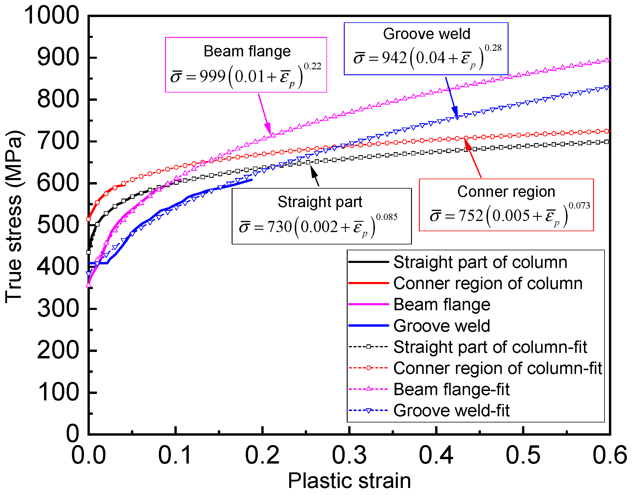
| Specimen Region | Young’s Modulus E (MPa) | Yield Strength σy0 (MPa) | Ultimate Strength σu (MPa) | Hardening Exponent n | Fracture Strain under Tension |
|---|---|---|---|---|---|
| Straight part of the column | 2.06 × 10⁵ | 440.8 | 533.3 | 0.085 | 1.07 |
| Conner region of the column | 2.06 × 10⁵ | 511.0 | 570.6 | 0.073 | 1.03 |
| Beam flange plate | 2.06 × 10⁵ | 380.5 | 544.1 | 0.22 | 1.02 |
| Groove weld | 2.06 × 10⁵ | 380.1 | 491.3 | 0.28 | 1.33 |
Publisher’s Note: MDPI stays neutral with regard to jurisdictional claims in published maps and institutional affiliations. |
© 2022 by the authors. Licensee MDPI, Basel, Switzerland. This article is an open access article distributed under the terms and conditions of the Creative Commons Attribution (CC BY) license (https://creativecommons.org/licenses/by/4.0/).
Share and Cite
Li, W.; Jing, Y. A Simple Calibrated Ductile Fracture Model and Its Application in Failure Analysis of Steel Connections. Buildings 2022, 12, 1358. https://doi.org/10.3390/buildings12091358
Li W, Jing Y. A Simple Calibrated Ductile Fracture Model and Its Application in Failure Analysis of Steel Connections. Buildings. 2022; 12(9):1358. https://doi.org/10.3390/buildings12091358
Chicago/Turabian StyleLi, Wenchao, and Yuan Jing. 2022. "A Simple Calibrated Ductile Fracture Model and Its Application in Failure Analysis of Steel Connections" Buildings 12, no. 9: 1358. https://doi.org/10.3390/buildings12091358
APA StyleLi, W., & Jing, Y. (2022). A Simple Calibrated Ductile Fracture Model and Its Application in Failure Analysis of Steel Connections. Buildings, 12(9), 1358. https://doi.org/10.3390/buildings12091358