Macromechanical Failure Criteria: Elasticity, Plasticity and Numerical Applications for the Non-Linear Masonry Modelling

Abstract

Sometimes it is difficult to choose the most appropriate failure criterion for the problem analyzed. For brittle materials, attention must be paid to the availability of experimental data and the calibration of the representative parameters, within the chosen failure criterion. The work herein presented, starting with an overview on machromechanical failure criteria, analysed in the Haigh-Westergaard Stress Space, investigates the suitability of Mohr-Coulomb, Drucker-Prager and Concrete Damaged Plasticity failure criteria of masonry structures, underlining their specific characteristics and implementation in FEM simulations. The Pavia Door Wall experimental campaign under pseudo-static cyclic test is considered as benchmark study. The results of the experimental tests are compared with a FE model developed with ABAQUS computer program considering several failure criteria and equivalent frame approach. Among the investigated failure criteria Concrete Damaged Plasticity is able to capture the actual behaviour of the masonry walls under monotonic excitation. In particular, thanks to the adaptability of the Guo’s model in the definition and calibration of the uniaxial behavior, the model suitability in catching the variation of the cohesion and the evolution of the damage is better in comparison with the other addressed failure criteria.

1. Introduction

The failure criterion theory and its application in the framework of the structural analysis deserves a wide discussion based on the fundamental principles, models, and field of application. The structural design cannot neglect the analysis of the stresses, therefore, a correct evaluation of the state of the stresses in the structural elements is of paramount importance for a correct modelling and safety estimation [1]. The theory of elasticity and plasticity are the theoretical tool for the representation of natural phenomena belonging to the experimental observation of the macroscopic behaviour of a deformable solid. The theory of elasticity, in its mathematical form, is based on a linear relationship between deformation and tension through the material linear constitutive models. The major challenges reside in the large number of tensional configurations occurring in a deformable solid which promote the triggering of failure criteria, mathematically defined as hyper-surfaces representative of the allowed tensional states. Conversely, the theory of plasticity is an extension of the theory of elasticity accounting for the stress flow belonging to the plastic deformation occurring in the deformable solid. It is aimed at the identification of the constitutive relation between plastic deformation and tension. The extensions of the theory of plasticity to anisotropic materials, such as masonry, ground, reinforced concrete, has gained high interest in the last decades leading to the development of new criteria and specific theory. These theories are based on the mechanics of continuum, where the meaning of continuum identifies a body where points can be set as geometric entities of a regular domain of the space in which a density mass function can represent its measure. In this paper, reference is made to “Cauchy continuum theory” in which tension and deformations are a function of three spatial variables.

The main problem encountered in treating brittle materials, and specifically masonry, is the choice of a failure criterion more prone to an easy calibration of the uniaxial compression and uniaxial tension behaviour, starting from experimental data and parameters obtained through tests carried out in situ [2,3]. Among the possible failure criteria present in the literature several works demonstrated that the Concrete Damaged Plasticity Model (CDP) is easily adaptable to all the material having brittle behaviour such as masonry, but these claims have hardly been validated by comparison with experimental tests on entire wall panels or entire masonry structures [4,5,6]. Another model which can be used for the definition of the macromechanical behaviour of the brittle anisotropic materials is the Drucker Prager (DP) [7,8,9,10,11] whose main lack is the loosing of accuracy in presence of large displacement as the model is not able to catch the variation of the cohesion as a function of the plastic deformation.

The aim of the present work is to provide a suggestion in terms of theoretical and applicative tools for the choice of the appropriate macromechanical failure criteria for the modelling of masonry walls.

The models to calibrate the uniaxial behavior in traction and compression typical of brittle materials are presented in detail. The calibration is also applied to a specific case of masonry wall, whose data and tests are available in the literature. Moreover, the so-called Pavia Door Wall experimental campaign [10] is selected has benchmark study and the experimental are compared with a FEM model developed in ABAQUS. A comparison with a frame equivalent model [6] is also proposed.

In detail, in Section 2 the properties of the Haigh-Westergaard Stress Space are recalled. In Section 3 the description of the failure criteria is reported. In Section 4 the case study of the Pavia door Wall is described, and the FEM simulations are reported with reference to Drucker Prager (DP) material modelling and Concrete Damage Plasticity (CDP). In the same section, the comparison with the experimental tests and model based on the equivalent frame are reported. Section 5 includes the conclusions and the main remarks and future developments.

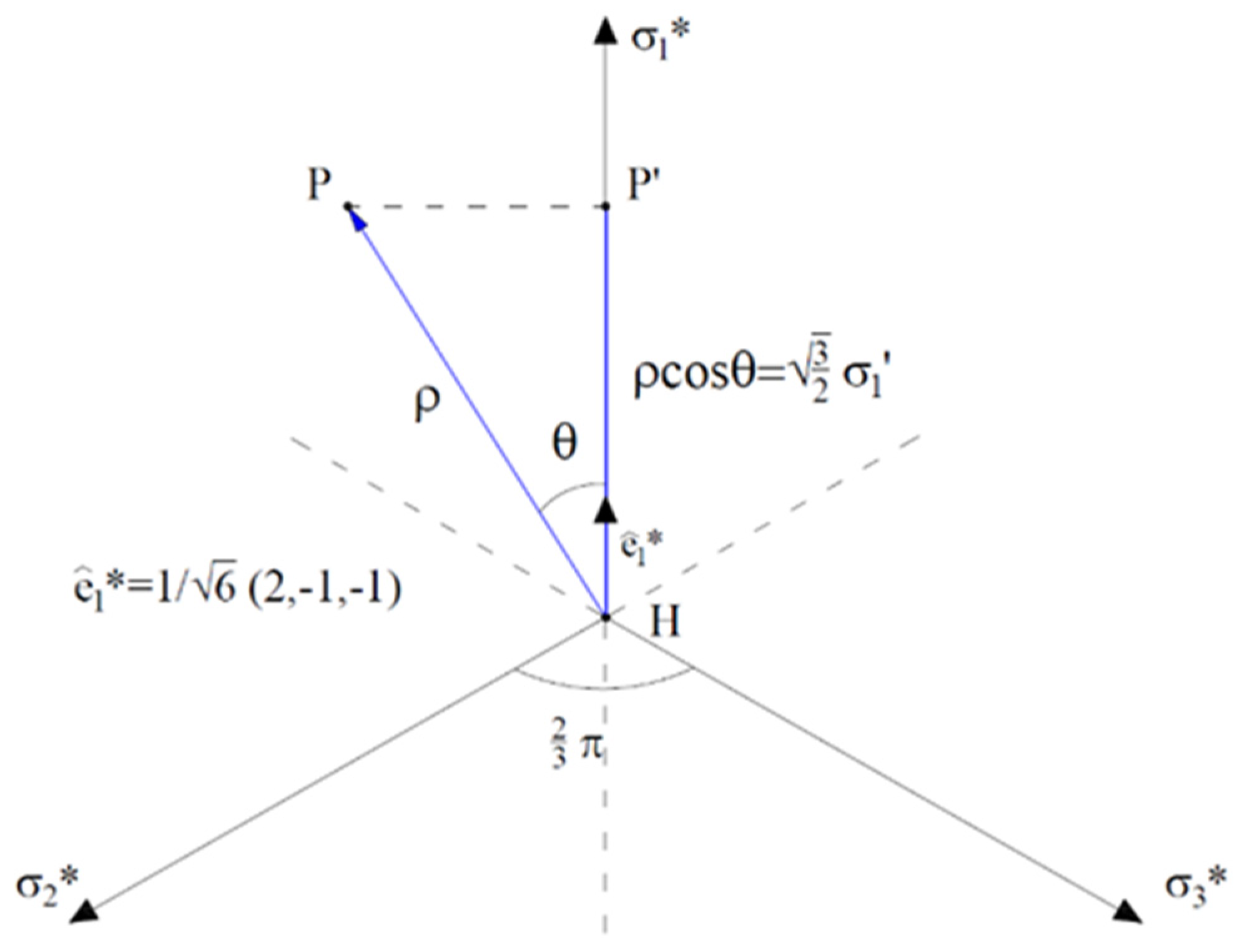
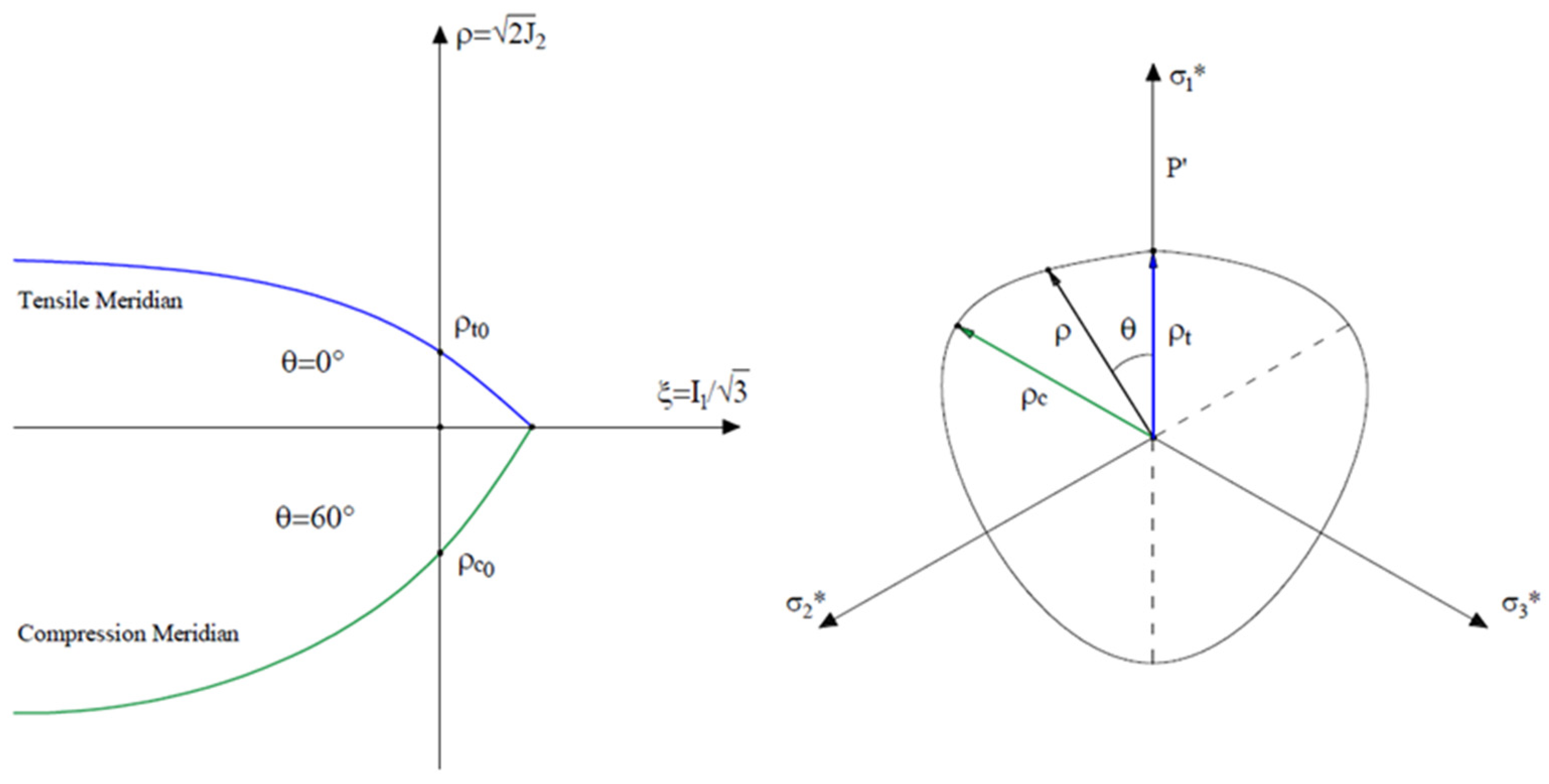
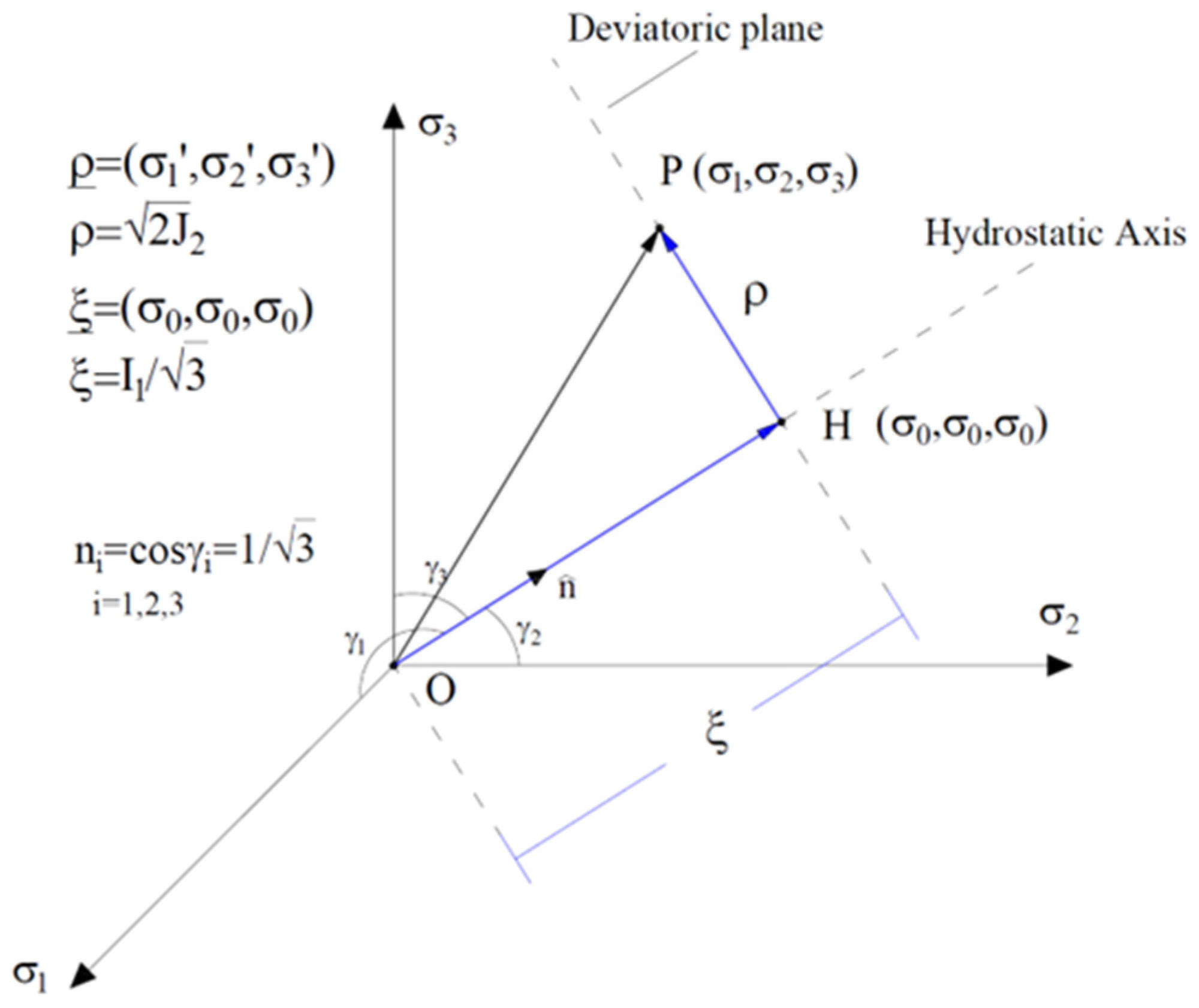
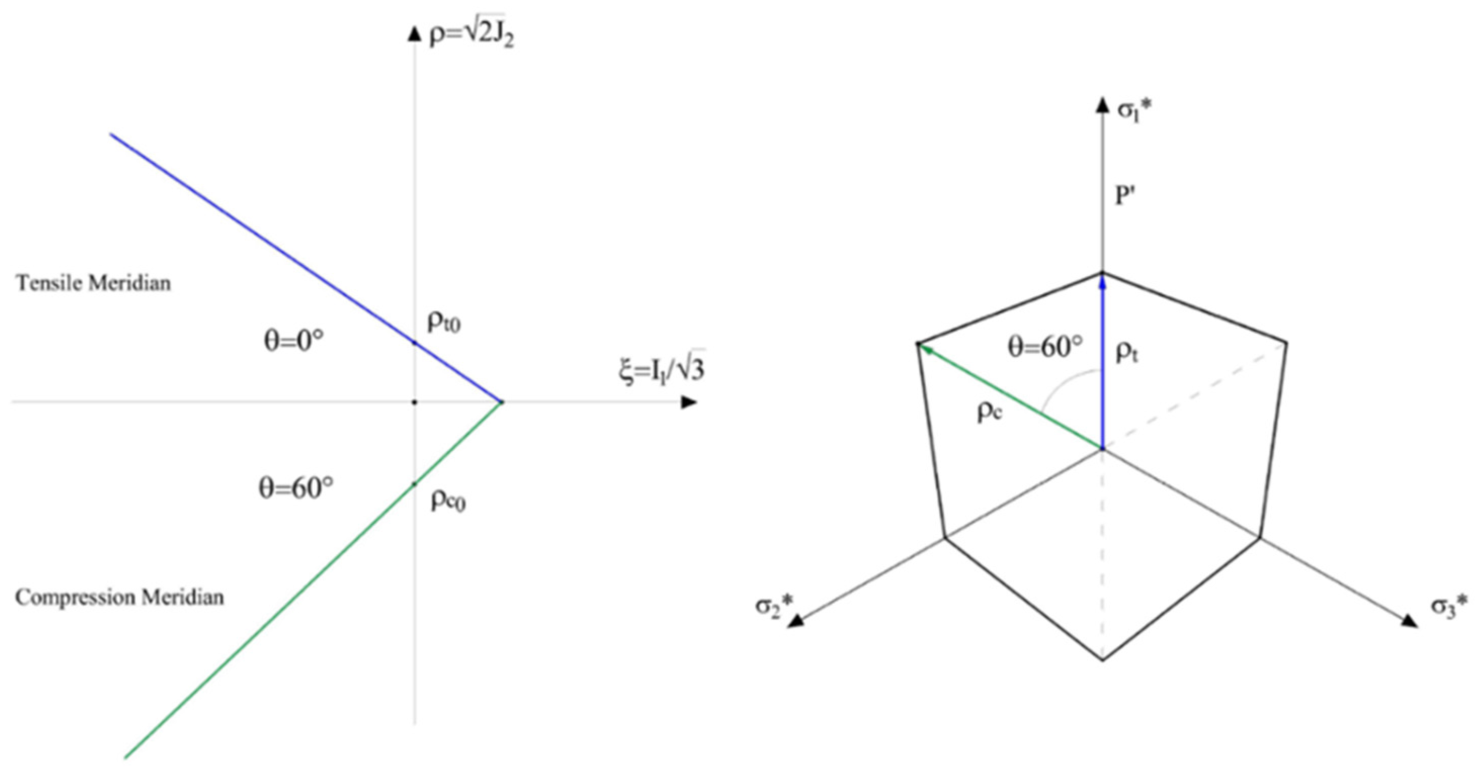
2. Meridian and Deviatoric Plane: Haigh-Westergaard Stress Space

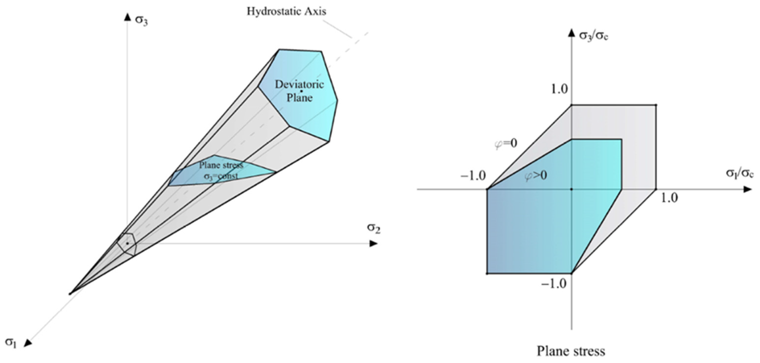
The space of tension of Haigh-Westergaard (H-W) (Figure 1) allows a geometrical representation of the tensional condition of a point P and it is fundamental for the theory of plasticity and failure criteria [11,12,13]. As it is known the tensional state of a solid, in a point P, can be defined by the six components of tension $\left\{{\sigma }_{11},{\sigma }_{22},{\sigma }_{33},{\tau }_{12},{\tau }_{23},{\tau }_{31}\right\}$ and this imply geometrically the representation of a hyperspace with 6 dimensions. For isotropic materials, it is possible to represent the tensional condition by the only principal components $\left\{{\sigma }_1,{\sigma }_2,{\sigma }_3\right\}$ being the material response independent of the orientation of the reference system.

The H-W space of tensions, therefore, considers the three main stresses as coordinates suitable to represent the stress state in a point P of the solid. It should be considered that this representation provides a geometric conformation of the resistance domain, regardless of the orientation of the main reference system. Consequently, two coincident points in the space of H-W could be characterized by a different orientation of the principal axes. Let us consider a point P representative of a generic tensional condition and the corresponding position vector $\underset{\_}{OP}$ with components $\left\{{\sigma }_1,{\sigma }_2,{\sigma }_3\right\}$. This vector can be projected onto the hydrostatic axis, obtaining the vector $\underset{\_}{\xi }=\underset{\_}{OH}$, passing through the origin, equi-inclined with respect to the reference system considered and therefore representative of the spherical component of the stress state P. The vector ξ can be expressed as:

$$\underset{\_}{\xi }=\left({\sigma }_0,{\sigma }_0,{\sigma }_0\right)\widehat{n} where {\sigma }_0=\frac{{\sigma }_1+{\sigma }_2+{\sigma }_3}{3}=\frac{I_1}{3}$$

(1)

considering that:

$$\left|OH\right|=\underset{\_}{OP} · \widehat{n}=\left({\sigma }_1,{\sigma }_2,{\sigma }_3\right)·\left(1/\sqrt{3},1/\sqrt{3},1/\sqrt{3}\right)$$

(2)

the modulus $\xi$ is given by the following relation:

$$\xi =I_1/\sqrt{3}$$

(3)

Each plane orthogonal to the segment $\underset{\_}{OH}$ and the vector $\underset{\_}{\xi }$ is a deviatoric plane, whose distance from the axis is identified precisely by the entity of ξ. Analytically, it is possible to confirm the deviatoric nature of the plane orthogonal to OH by operating through the vector difference between the position vector OP, representative of the total stress state, and the vector $\underset{\_}{\xi }=\underset{\_}{OH}$, representative of the spherical part of the tension:

$$\underset{\_}{\rho }=\underset{\_}{HP}=\underset{\_}{OP}-\underset{\_}{OH}=\left({\sigma }_1,{\sigma }_2,{\sigma }_3\right)-\left({\sigma }_0,{\sigma }_0,{\sigma }_0\right)=\left({\sigma }_1^{\prime },{\sigma }_2^{\prime },{\sigma }_3^{\prime }\right)$$

(4)

where ${\sigma }_1^{\prime },{\sigma }_2^{\prime },{\sigma }_3^{\prime }$ represent the deviatoric components of the tensor of tensions $\stackrel{=}{T}$. The length ρ, is equal to the modulus of the vector $\underset{\_}{\rho }=\underset{\_}{HP}$, given by:

$$\rho =\left|HP\right|=\sqrt{{{\sigma }_1^{\prime }}^2+{{\sigma }_2^{\prime }}^2+{{\sigma }_3^{\prime }}^2}=\sqrt{2J_2}$$

(5)

This relationship can be obtained from the second invariant $J_2=\frac{1}{3}{I}_1{}^2+I_2=\frac{1}{6}\left[{\left({\sigma }_1-{\sigma }_2\right)}^2+{\left({\sigma }_2-{\sigma }_3\right)}^2+{\left({\sigma }_3-{\sigma }_1\right)}^2\right]$ rewritten as a function of the deviatoric components ${\sigma }_1^{\prime },{\sigma }_2^{\prime },{\sigma }_3^{\prime }$. The result obtained highlights the similarity deriving from the comparison between the triangles generated respectively by the orthogonal and tangential components of the octahedral tension $\left({\sigma }_{oct}=(1/3)I_1,{\mathsf{\tau }}_{oct}=\sqrt{(2/3)J_2}\right)$ and the spherical and deviatoric components in the H-W plane (ξ, ρ).

The component $\rho$ has is proper orientation $\theta$ in the deviatoric plan (Figure 2) where axes ${\sigma }_1{}^{*},{\sigma }_2{}^{*},{\sigma }_3{}^{*}$ are the projection of the system ${\sigma }_1,{\sigma }_2,{\sigma }_3$ on the deviatoric plane. The purpose is to express the principal tensions with reference to coordinates $\xi , \rho ,\theta$ which consent to describe the failure surface as a function of sections, rotating around the hydrostatic axis. First of all, it is needed to determine the projection of the vector $\underset{\_}{\rho }=\underset{\_}{HP}$ on the axis ${\sigma }_1{}^{*}$ whose unitary vector ${\widehat{e}}_1{}^{*}$ has components $\left(m_1,m_2,m_3\right)=\left(2/\sqrt{6},-1/\sqrt{6},-1/\sqrt{6}\right)$. This could be demonstrated by stating that ${\widehat{e}}_1$ lies on the same plane defined by the hydrostatic axis ${\sigma }_1$. Given the orthogonality of ${\widehat{e}}_1{}^{*}$ with respect to the hydrostatic axis, the first director cosine $m_1(2/\sqrt{6})$ will be the complement of $n_1=1/\sqrt{3}$ in the resulting right triangle. Considering the symmetry of ${\sigma }_1{}^{*}$ with respect to the other two axes ${\sigma }_2{}^{*},{\sigma }_3{}^{*}$, we can obtain the other two components of equal value of the unit vector ${\widehat{e}}_1{}^{*}$ which will be $m_2=m_3=-1/\sqrt{6}$.

The projection of the vector $\underset{\_}{\rho }=\underset{\_}{HP}$ on the axis ${\sigma }_1{}^{*}$ is given by:

$$P^{\prime }=\rho cos\theta =\underset{\_}{HP}·{\widehat{e}}_1{}^{*}=\left({\sigma }_1^{\prime },{\sigma }_2^{\prime },{\sigma }_3^{\prime }\right)·\left(\frac{2}{\sqrt{6}},-\frac{1}{\sqrt{6}},-\frac{1}{\sqrt{6}}\right)$$

(6)

$$\rho cos\theta =\frac{1}{\sqrt{6}}\left(2{\sigma }_1^{\prime }-{\sigma }_2^{\prime }-{\sigma }_3^{\prime }\right)$$

(7)

and considering that $-{\sigma }_1^{\prime }={\sigma }_2^{\prime }+{\sigma }_3^{\prime } ,$ because of the definition of deviatoric stress, it is possible to write:

$$\rho cos\theta =\sqrt{\frac{3}{2}}{\sigma }_1^{\prime }$$

(8)

By substituting Equation (5) into (8) it is obtained:

$$cos\theta =\frac{\sqrt{3}}{2}\frac{{\sigma }_1^{\prime }}{\sqrt{J_2}}$$

(9)

And:

$${\sigma }_1^{\prime }=\frac{2}{\sqrt{3}}\sqrt{J_2} cos\theta$$

(10)

In a similar way, the relations linking the other deviatoric components of the tension ${\sigma }_2^{\prime },{\sigma }_3^{\prime }$ to the angle θ can be obtained, considering an equal subdivision of the sectors defined by the axes of the reference system for an angle equal to 2π/3. From Figure 2 it results:

$${\sigma }_2^{\prime }=\frac{2}{\sqrt{3}}\sqrt{J_2} cos\left(\frac{2\pi }{3}-\theta \right)$$

(11)

$${\sigma }_3^{\prime }=\frac{2}{\sqrt{3}}\sqrt{J_2} cos\left(\frac{2\pi }{3}+\theta \right)$$

(12)

These relations are valid for values of θ between 0 and π/3 and therefore applicable to the whole domain by symmetry with respect to the sector of amplitude equal to π/3. By adding the hydrostatic component to the deviatoric component, it is possible to obtain equations that relate the three main stresses ${\sigma }_1,{\sigma }_2,{\sigma }_3$ with the coordinates $\xi ,\rho ,\theta$:

$$\left\{\begin{array}{c}{\sigma }_1\\ {\sigma }_2\\ {\sigma }_3\end{array}\right\}=\frac{1}{\sqrt{3}} \left\{\begin{array}{c}\xi \\ \xi \\ \xi \end{array}\right\}+\sqrt{\frac{2}{3}}\rho \left\{\begin{array}{c}cos\theta \\ cos\left(\frac{2\pi }{3}-\theta \right)\\ cos\left(\frac{2\pi }{3}+\theta \right)\end{array}\right\}$$

(13)

These relations can be expressed as a function of the invariants $I_1,J_2$:

$$\left\{\begin{array}{c}{\sigma }_1\\ {\sigma }_2\\ {\sigma }_3\end{array}\right\}=\frac{1}{3} \left\{\begin{array}{c}{I}_1\\ I_1\\ I_1\end{array}\right\}+\frac{2}{\sqrt{3}}\sqrt{J_2} \left\{\begin{array}{c}cos\theta \\ cos\left(\frac{2\pi }{3}-\theta \right)\\ cos\left(\frac{2\pi }{3}+\theta \right)\end{array}\right\}$$

(14)

3. Failure Criteria

The failure criteria define the elastic limit of a material subjected to a complex stress state [8,9,13]. The fundamental problem is to relate the critical parameters of the material obtained with simple uniaxial tests, with the resistance of the material subjected to multiaxial stress regimes. The result is the definition of a hypersurface $\partial \mathsf{\Gamma }$, boundary of a domain Γ, in the space of the independent components of the stress tensor $\stackrel{=}{T}$. These components, for convenience, can be arranged in the vector $\underset{\_}{\sigma }$. We therefore define a yield function, dependent on the state of point stress $f\left(\underset{\_}{\sigma }\left(\underset{\_}{X}\right)\right)$. This function can be expressed in a general way as:

$$f\left(\underset{\_}{\sigma }\right)=f\left({\sigma }_{ij},k_1,k_2,\dots ,k_n\right)=0$$

(15)

where $k_1,k_2,\dots ,k_n$ they are constants of the material to be experimentally determined as a function of the resistances defined by uniaxial tests.

For isotropic materials, since the orientation of the main system with respect to a generic Cartesian system orthogonal on the mechanical response of the material is irrelevant, the function $f\left(\underset{\_}{\sigma }\right)$ can be uniquely expressed through only the main components of the stresses ${\sigma }_1,{\sigma }_2,{\sigma }_3$. Consequently, Equation (15) can be replaced with:

$$f\left(\underset{\_}{\sigma }\right)=f\left({\sigma }_{1,}{\sigma }_2,{\sigma }_3,k_1,k_2,\dots ,k_n\right)=0$$

(16)

The principal stresses ${\sigma }_{1,}{\sigma }_2,{\sigma }_3$ and therefore the deviatoric stresses ${\sigma }_1^{\prime },{\sigma }_2^{\prime },{\sigma }_3^{\prime }$, can be expressed as a combination of the invariants $I_1,J_2,J_3$. Consequently, it is possible to write the function f(σ) as follows:

$$f\left(\underset{\_}{\sigma }\right)=f\left(I_1,J_2,J_3,k_1,k_2,\dots ,k_n\right)=0$$

(17)

This expression has the advantage of having the three invariants as directly correlated to the Haigh-Westergaard coordinates ($\xi ,\rho ,\theta )$ which allow analysing, in a direct way, the stress state on the meridians and in the deviatoric plane of the domain. In this case, the plasticity function can be written as follows:

$$f\left(\underset{\_}{\sigma }\right)=f\left(\xi ,\rho ,\theta ,k_1,k_2,\dots ,k_n\right)=0$$

(18)

3.1. Failure Criteria Independent of the Hydrostatic Pressure

The plasticity surface can follow additional hypotheses resulting from experimental observation. For metals, the experimental evidence highlighted the independence of $f\left(\underset{\_}{\sigma }\right)$ from the hydrostatic component of the stress tensor. The absence of the spherical part of the stress tensor results in a yield function of the type:

$$f\left(\underset{\_}{\sigma }\right)=f\left(J_2,J_3,k_1,k_2,\dots ,k_n\right)=0$$

(19)

in which the dependence on the first invariant of the stress tensor $I_1$ disappears. This is the case of the criteria of Von Mises and Tresca, which is particularly used for the study of metallic materials and implemented in all the best codes of finite element calculation (FEM).

3.2. Failure Criteria Dependent on the Hydrostatic Pressure

The mechanical behaviour of many non-metallic materials such as soils, rocks, but also concrete and masonry, is linked to resistant frictional phenomena dependent on the hydrostatic component of the stress tensor. Consequently, the breaking surface, which can be expressed in forms $f\left(\underset{\_}{\sigma }\right)=f\left(I_1,J_2,J_3,k_1,k_2,\dots ,k_n\right)=0$ or $f\left(\underset{\_}{\sigma }\right)=f\left(\xi ,\rho ,\theta ,k_1,k_2,\dots ,k_n\right)=0$, will be dependent on the first invariant $I_1$ or on the coordinate $\xi$. In addition, to describe the surface in the three-dimensional space of tensions, a single deviatoric cross-section will not be sufficient, given the variability of this along the hydrostatic axis. From this perspective, the study of surface meridians in the meridian plane is fundamental $\xi ,\rho$ varying the angle $\theta$. For isotropic materials, the conformation of the deviatoric section is characterized by triple symmetry, as shown in Figure 3. Consequently, both experimental and analytical characterization can be carried out on the single sector with an angle θ between 0° and 60°.

By sorting the principal tension by ${\sigma }_1>{\sigma }_2>{\sigma }_3$, it is possible to identify the following limit cases:

$${\sigma }_1={\sigma }_2>{\sigma }_3$$

(20)

$${\sigma }_1>{\sigma }_2={\sigma }_3$$

(21)

corresponding to the sectors $\theta =60°$ and $\theta =0°$, respectively. The meridian corresponding to the angle $\theta =60°$ is called “meridian of compression”, being characterized by compressive stress superimposed on the spherical stress state, in one direction, while the meridian corresponding to $\theta =0°$ is called “meridian of traction” being characterized by tensile stress superimposed on the deviatoric stress state, in one direction.

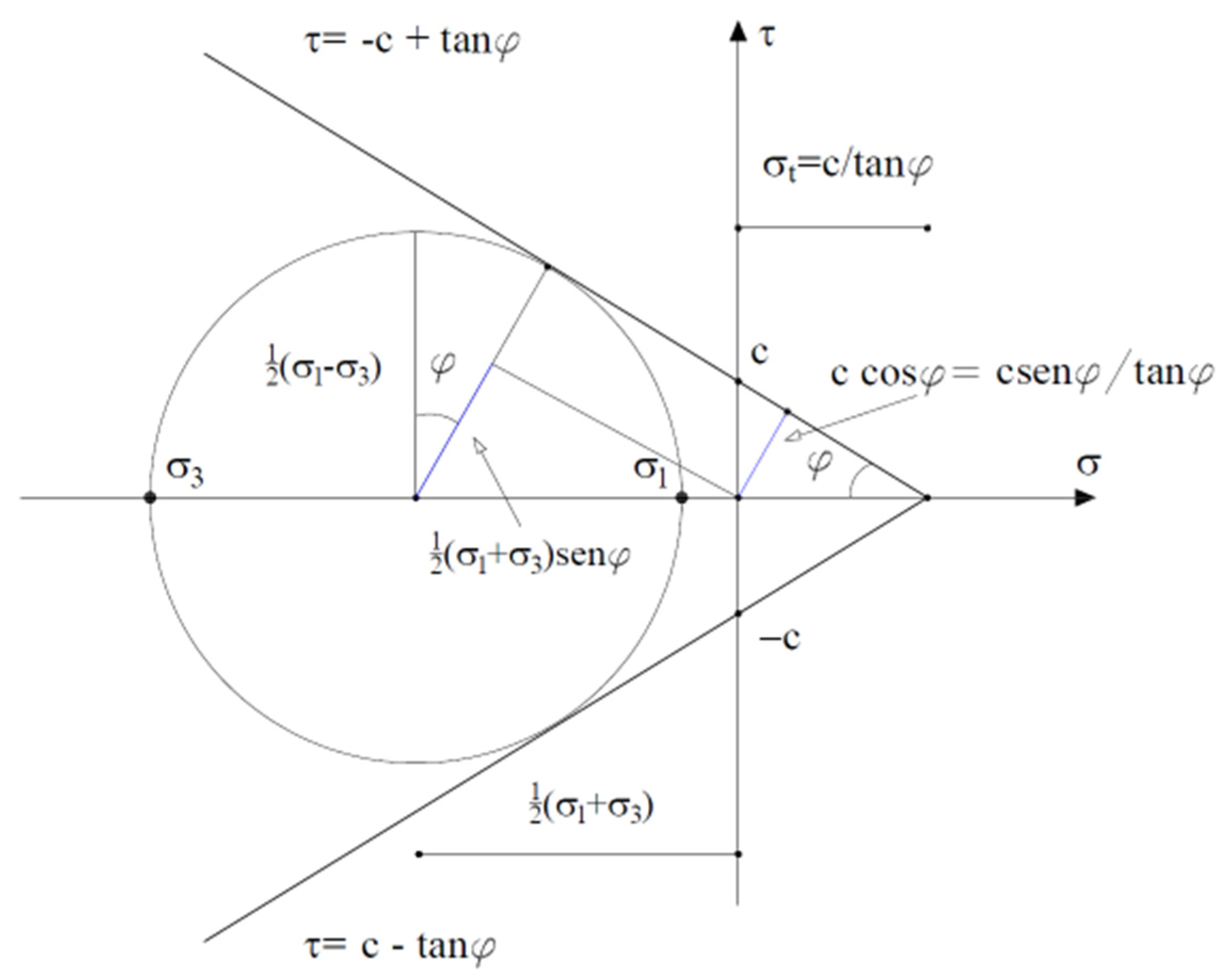
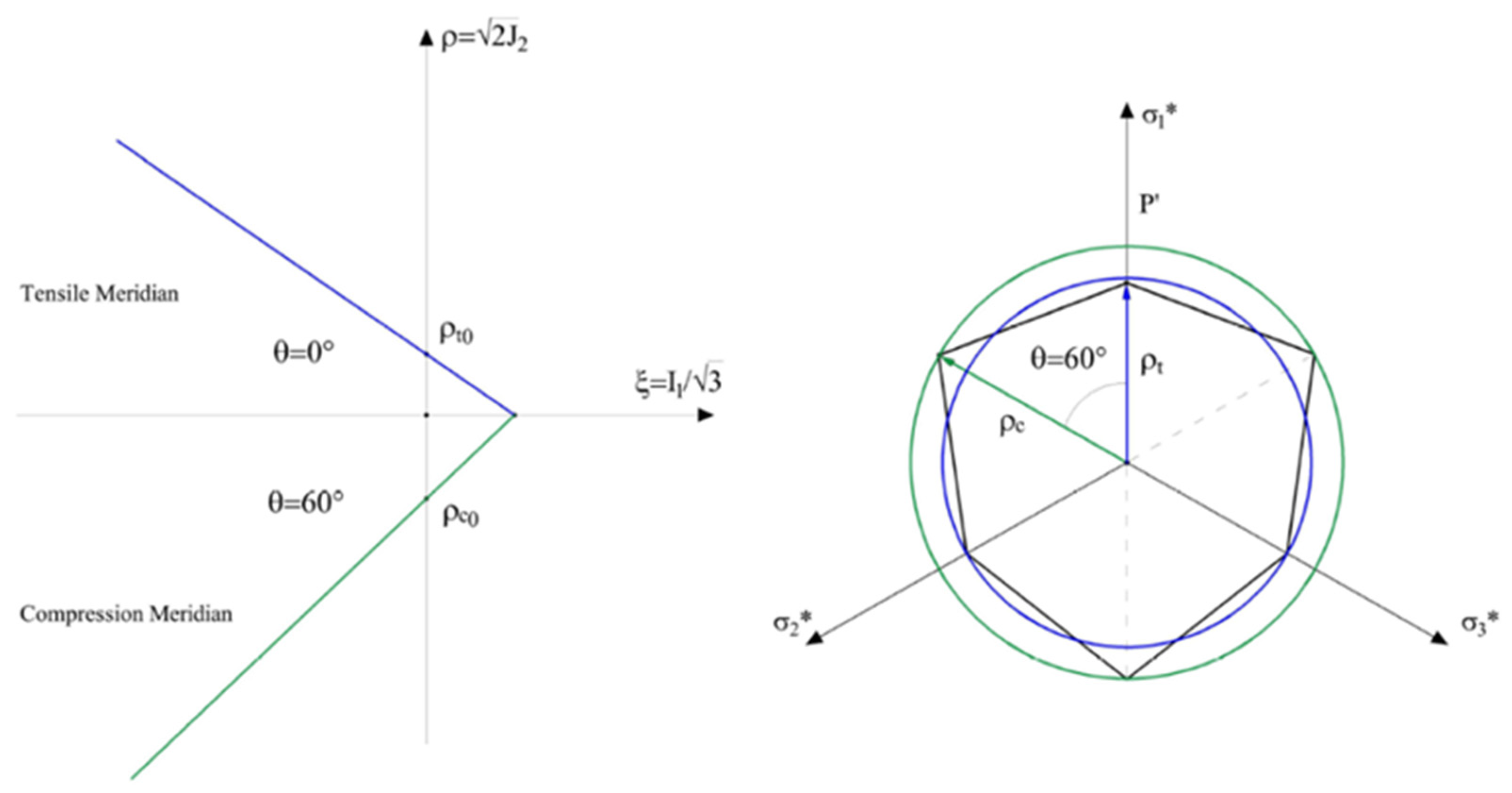
3.2.1. Mohr-Coulomb Failure Criterion

The Mohr-Coulomb failure criterion, also called the internal friction criterion, can be seen as a generalization of the Tresca criterion [13]. Both identify the cause of the failure in reaching the maximum shear stress, but in the first case, the limit value is constant, while in the second the limit shear stress is a function of the normal stress ${\sigma }_0$. Consequently, it can be assumed that the crisis occurs when, fixed a value of the normal stress ${\sigma }_0$ on a plane, the tangential stress reaches the value:

$$\left|\tau \right|=c-{\sigma }_0 tan\phi$$

(22)

where c is the cohesion and $\phi$ is the internal friction angle (Figure 4); both are constants of the material to be determined experimentally.

Referring to a pluriaxial stress state, it is evident that the maximum value of the tangential stress τ is drawn from the plane representative of the greater of the three Mohr circles. Sorting the main stresses so that it turns out ${\sigma }_1>{\sigma }_2>{\sigma }_3$, ${\sigma }_1$ and ${\sigma }_3$ are respectively maximum and minimum main tension and the representative circle is the one characterized by a radius equal to $\raisebox{1ex}{$1$}\!\left/ \!\raisebox{-1ex}{$2$}\right.\left({\sigma }_1-{\sigma }_3\right)$. For the considerations and assumptions made, the influence of the intermediate main stress is excluded ${\sigma }_2$.

From Figure 4 the radius of the circle can also be expressed as:

$$R=\tau =(-\frac{ {\sigma }_1+{\sigma }_3}{2}+\frac{c}{tan\phi }) sen\phi$$

(23)

where $\frac{c}{tan\phi }={\sigma }_t$. The failure criterion can therefore be rewritten in the following form:

$$\frac{ {\sigma }_1-{\sigma }_3}{2}=-\frac{ {\sigma }_1+{\sigma }_3}{2}sen\phi +c cos\phi$$

(24)

The equations of six planes can be defined in the space of principal stresses ${\sigma }_1,{\sigma }_2,{\sigma }_3$, whose envelope is a pyramid with a vertex in the point ${\sigma }_1={\sigma }_2={\sigma }_3={\sigma }_t$, representative of the triaxial tensile strength and axis coinciding with the hydrostatic axis. Considering all the possible differences we obtain:

$${\sigma }_1-{\sigma }_3=\mp ({\sigma }_1+{\sigma }_3)sen\phi \pm 2c cos\phi$$

(25)

$${\sigma }_1-{\sigma }_2=\mp ({\sigma }_1+{\sigma }_2)sen\phi \pm 2c cos\phi$$

(26)

$${\sigma }_2-{\sigma }_3=\mp ({\sigma }_2+{\sigma }_3)sen\phi \pm 2c cos\phi$$

(27)

From Equation (24) further information can be obtained, for example by referring to the limit circles corresponding to the uniaxial tensional states of traction and compression (${\sigma }_1={\sigma }_t,{\sigma }_3=0; {\sigma }_1=0,{\sigma }_3={\sigma }_c)$. Highlighting the main tensions in the (24) it consequences that:

$${\sigma }_1\left(1+sen\phi \right)-{\sigma }_3\left(1-sen\phi \right)=2c cos\phi$$

(28)

and, therefore:

$${\sigma }_1\frac{\left(1+sen\phi \right)}{2c cos\phi }-{\sigma }_3\frac{\left(1-sen\phi \right)}{2c cos\phi }=1$$

(29)

from which results:

$${\sigma }_t=\frac{2c cos\phi }{1+sen\phi }$$

(30)

$${\sigma }_c=\frac{2c cos\phi }{1-sen\phi }$$

(31)

Consequently, Equation (29) can be rearranged in the form:

$$\frac{{\sigma }_1}{{\sigma }_t}-\frac{{\sigma }_3}{{\sigma }_c}=1$$

(32)

from which it is deduced the dependence of the conformation of the domain, in the case of a plane state of tension (in the specific case ${\sigma }_1,{\sigma }_3)$ from the relationship between the monoaxial tensions of traction and compression $m=\raisebox{1ex}{${\sigma }_c$}\!\left/ \!\raisebox{-1ex}{${\sigma }_t$}\right.$, as reported in Figure 5. From Figure 5, it is observed that for values of $m$ equal to 1, the Tresca criterion and the Mohr-Coulomb criterion are coincident and defined by the same symmetrical hexagon with respect to the bisectors of the orthogonal reference system considered.

The equation of the failure surface in the stress space can also be rewritten as a function of the invariants $I_1,J_2$ and of the angle θ or also in the coordinates $\xi ,\rho ,\theta$ remembering that $\xi ,\rho$ represent the axes of the plane of meridians. To do this, Equations (13) and (14) can be substituted in Equation (28), obtaining:

$$f\left(I_1,J_2,\theta \right)=\frac{1}{3}{I}_{1}sin\phi +\sqrt{J_2} sin\left(\theta +\frac{\pi }{3}\right)+\frac{\sqrt{J_2}}{\sqrt{3}}cos\left(\theta +\frac{\pi }{3}\right)sin\phi -c cos\phi =0$$

(33)

$$f\left(\xi ,\rho ,\theta \right)=\sqrt{2}\xi sin\phi +\sqrt{3}\rho sin\left(\theta +\frac{\pi }{3}\right)+\rho cos\left(\theta +\frac{\pi }{3}\right)sin\phi -\sqrt{6}c cos\phi =0$$

(34)

where $0\le \theta \le \frac{\pi }{3}$.

These relations are able to represent the irregular pyramid with a hexagonal base, exploiting the symmetry of the domain, making it sufficient to study a single sector of $60°$. Once the apex of the pyramid is known, with coordinates ${\sigma }_1={\sigma }_2={\sigma }_3={\sigma }_t$, it is sufficient to define the deviatoric section for ξ, defined by the radii ${\rho }_{t_0}$ and ${\rho }_{c_0}$ obtained through the intersection of the meridians in traction and compression with the axis of equation $\xi =0$.

By considering that $\xi =0, \theta =0°$ and $\xi =0, \theta =60°$ in the Equation (34):

$${\rho }_{t_0}=\frac{2\sqrt{6}c cos\phi }{3+sin\phi }$$

(35)

$${\rho }_{c_0}=\frac{2\sqrt{6}c cos\phi }{3-sin\phi }$$

(36)

and the ratio of these lengths (also called flow stress ratio) is given by:

$$K_c=\frac{{\rho }_{t_0}}{{\rho }_{c_0}}=\frac{3-sin\phi }{3+sin\phi }$$

(37)

The ratio ${\rho }_{t_0}/{\rho }_{c_0}$ is fundamental for the Drucker-Prager criterion to calibrate the parameters on the base of those characterising the Mohr-Coulomb criterion (Figure 6).

3.2.2. Drucker-Prager Failure Criterion

To exploit the analytical and computational advantages of a representation of the breaking domain via a regular surface, the Drucker-Prager (DP) criterion was formulated in 1952, which can be seen as a generalized version of the Von Mises criterion, in which the dependence on the hydrostatic component of the stress tensor is manifested by adding a term to the relation proposed by Von Mises [11,13]. Consequently, the criterion can be written in the following form:

$$f\left(I_1,J_2\right)=\alpha I_1+\sqrt{J_2}-k=0$$

(38)

or by using the variables $\xi ,\rho$ as:

$$f\left(I_1,J_2\right)=\sqrt{6}\alpha \xi +\rho -\sqrt{2}k=0$$

(39)

where $\alpha$ and k depend on the material and must be determined experimentally. If the parameter $\alpha$ is equal to 0 the criterion coincides with the Von Mises one. In terms of main stresses, the criterion can be written in the following form:

$$\sqrt{\frac{1}{6}\left[{\left({\sigma }_1-{\sigma }_2\right)}^2+{\left({\sigma }_2-{\sigma }_3\right)}^2+{\left({\sigma }_3-{\sigma }_1\right)}^2\right]}+\alpha \left(\frac{ {\sigma }_1+{\sigma }_2+{\sigma }_3}{3}\right)=k$$

(40)

The relationship defines a cone with a vertex at the point in the principal coordinate space ${\sigma }_1={\sigma }_2={\sigma }_3=\frac{k}{\alpha }$ and characterized by circular sections on the deviatoric planes with radii linearly dependent on the hydrostatic tension (Figure 7). The parameters $\alpha$ e k can be related to the monoaxial tension state in traction and compression according to the following relations:

$${\sigma }_t=\frac{3k}{\sqrt{3}+\alpha }$$

(41)

$${\sigma }_t=\frac{3k}{\sqrt{3}+\alpha }$$

(42)

The second relationship, in particular, places limitations on the value assumed by the parameter α, which must be less than √3.

A fundamental parameter indicative of the asymmetry of the domain, for flat stress states, is the ratio $m$ between compression and uniaxial traction:

$$m=\frac{{\sigma }_c}{{\sigma }_t}=\frac{\sqrt{3}-\alpha }{\sqrt{3}+\alpha }$$

(43)

From the representation of a plane (biaxial) stress state, it is immediately possible to notice how for $m=1$ and therefore for $\alpha =0$, the criterion coincides with that of Von Mises.

3.2.3. Calibration of Drucker-Prager Parameters according to Mohr-Coulomb Criterion

Since the Drucker-Prager model turns out to be a smooth version of the Mohr-Coulomb criterion to avoid any numerical problems deriving from stress states located along the intersections of the faces constituting this domain, it may be useful to define the parameters of the Drucker model-Prager $\alpha ,k$ as a function of cohesion $c$ and the internal friction angle $\phi$ characterizing the Mohr-Coulomb criterion. Considering Equations (38) and (39), it is possible to obtain a Drucker-Prager failure surface that circumscribes or inscribes that of Mohr-Coulomb, as shown in the deviatoric section in Figure 8. In the first case, that is when the of Drucker-Prager is tangent to the outermost apexes of the Mohr-Coulomb hexagon, the two surfaces coincide along the compression meridian ${\rho }_c$, with $\theta =60°$. For ease of calculation, we consider the meridian radius ${\rho }_{c_0}$, characterized by $\xi =0$. Obtaining ${\rho }_{c_0}$ for θ = 60° and $\xi =0$ from Equation (39) and from equality with Equation (36) we obtain:

$$\alpha =\frac{2 sin\phi }{\sqrt{3}\left(3-sin\phi \right)}$$

(44)

$$k=\frac{6c cos\phi }{\sqrt{3}\left(3-sin\phi \right)}$$

(45)

If, on the other hand, the Drucker-Prager circle coincides with the innermost vertices of the Mohr-Coulomb hexagon, the two surfaces coincide along the meridian of traction ${\rho }_t$, with $\theta =0°$. Obtaining ${\rho }_{t_0}$ for $\theta =0°$ and $\xi =0$ from the Equation (39) and from equality with the Equation (35), it is possible to get:

$$\alpha =\frac{2 sin\phi }{\sqrt{3}\left(3+sin\phi \right)}$$

(46)

$$k=\frac{6c cos\phi }{\sqrt{3}\left(3+sin\phi \right)}$$

(47)

A further modification to the model can be made to make the adherence between the two breaking models even more effective and therefore the yield for more complex load paths. In this case, the Drucker-Prager criterion can also depend on the third invariant of the deviatoric stress tensor (Extended Drucker-Prager), obtaining a function of the type $f=f\left(I_1,J_2,J_3\right)$, which allows to obtain a deviatoric section passing through all the corners of the Mohr-Coulomb hexagon, as shown in Figure 9. The fracture surface and consequently its deviatoric section are dependent on the parameter $K_c=\frac{3-sin\phi }{3+sin\phi }$ called flow stress ratio, already explained above through the Equation (37) as the ratio between the meridians ${\rho }_{c_0}$, ${\rho }_{t_0}$. For $K_c=1$ (upper limit), the deviatoric section will coincide with the circle tangent to the external vertices of the Mohr-Coulomb hexagon, while for decreasing values of $K_c$, the section will have the shape shown in Figure 9 with increasingly sharp vertices. The value of $K_c$ will be limited below the value 0.778 (lower limit) to guarantee a breaking surface that is always convex.

In this case, the values of the parameters $\alpha ,k$ as a function of cohesion $c$ and the internal friction angle $\phi$ characterizing the Mohr-Coulomb criterion can be obtained under the following relations:

$$\alpha =\frac{tan\phi }{\sqrt{9+12{tan}^2\phi }}$$

(48)

$$k=\frac{3c}{\sqrt{9+12{tan}^2\phi }}$$

(49)

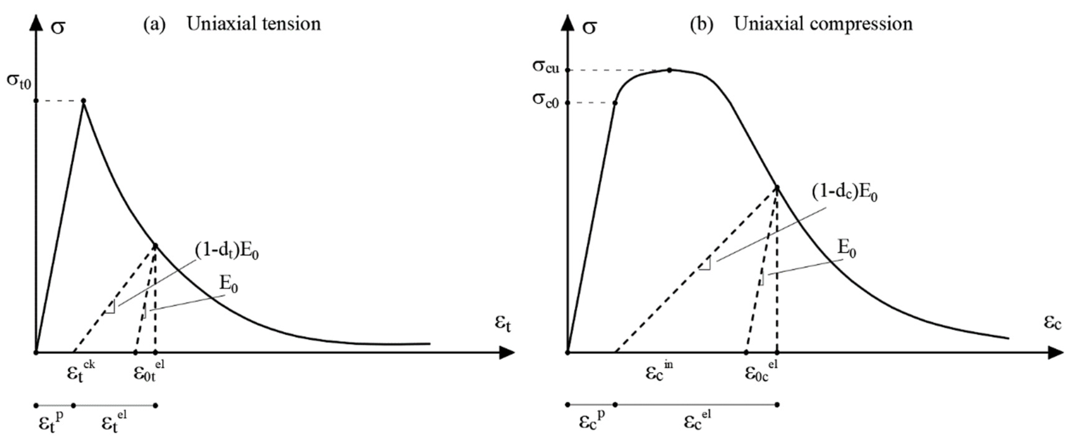
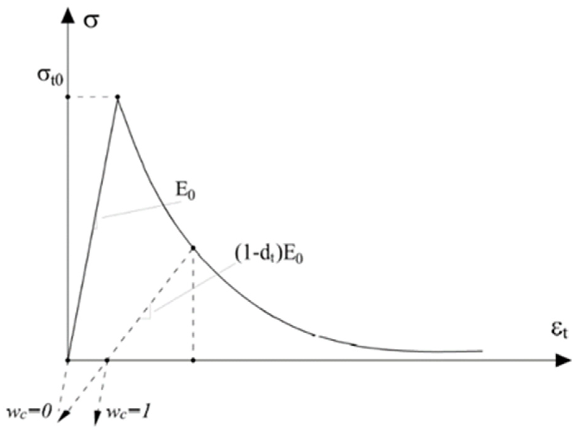
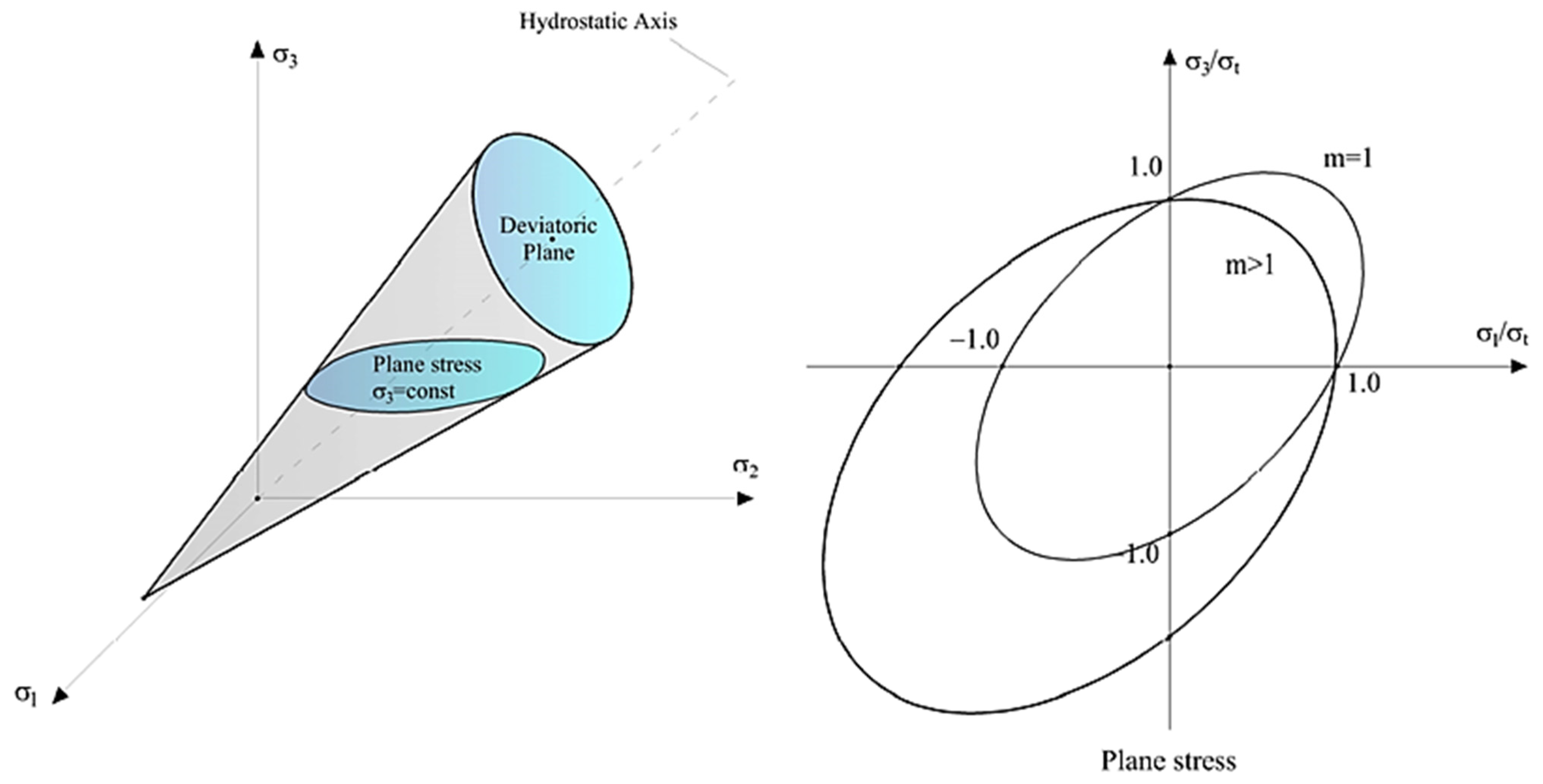
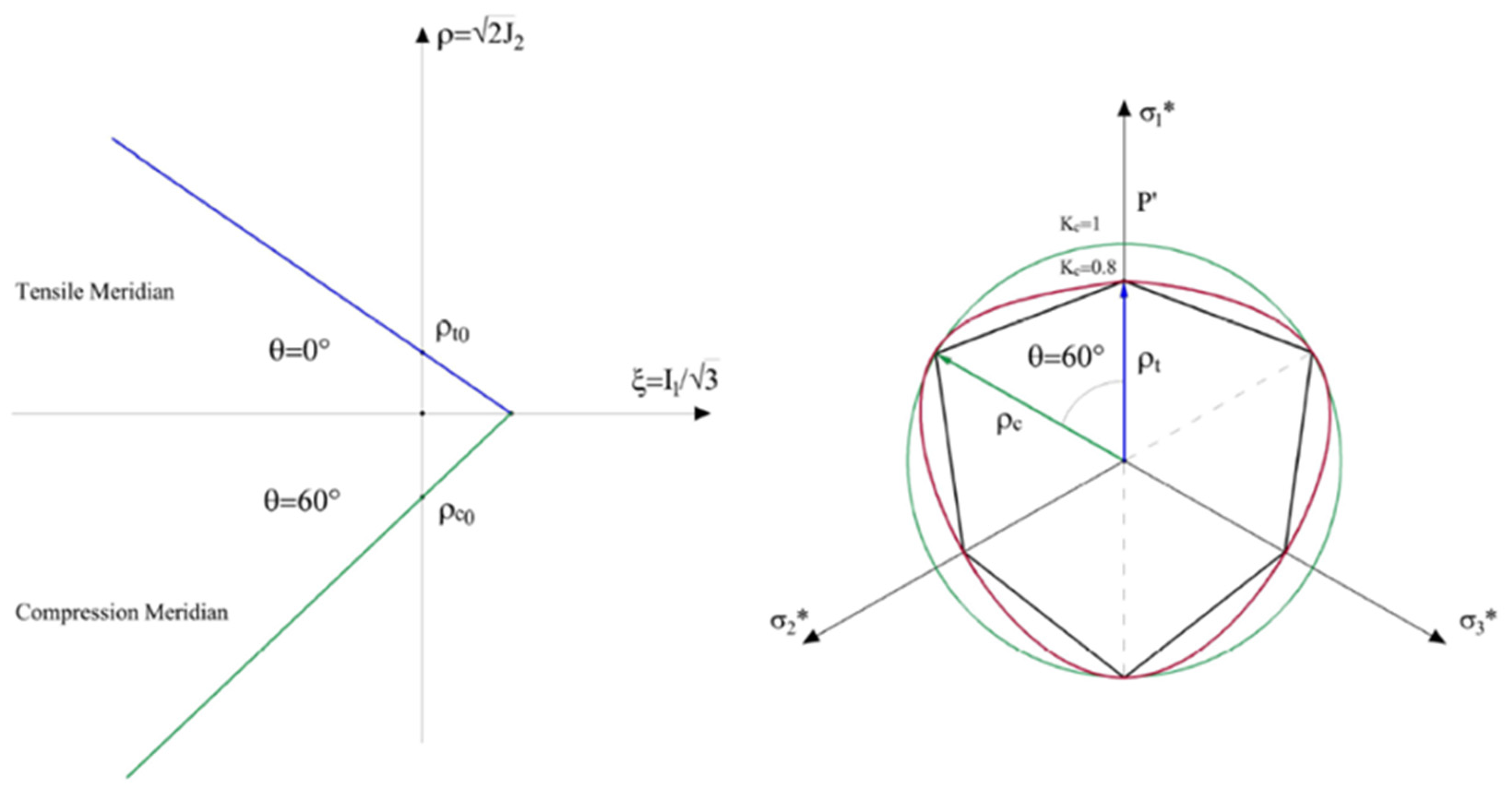
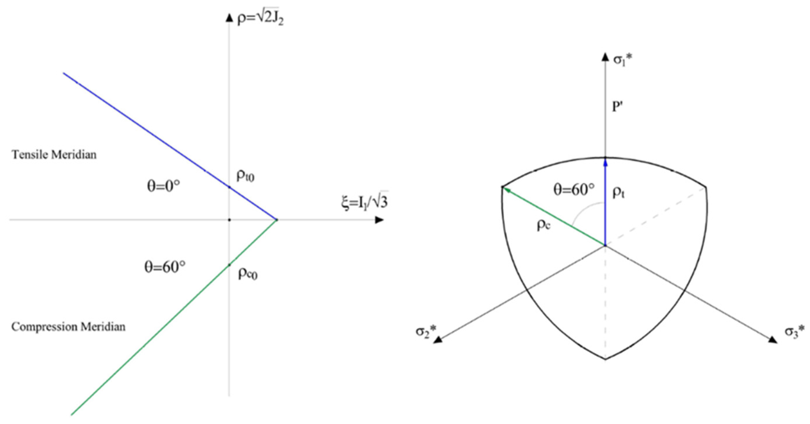
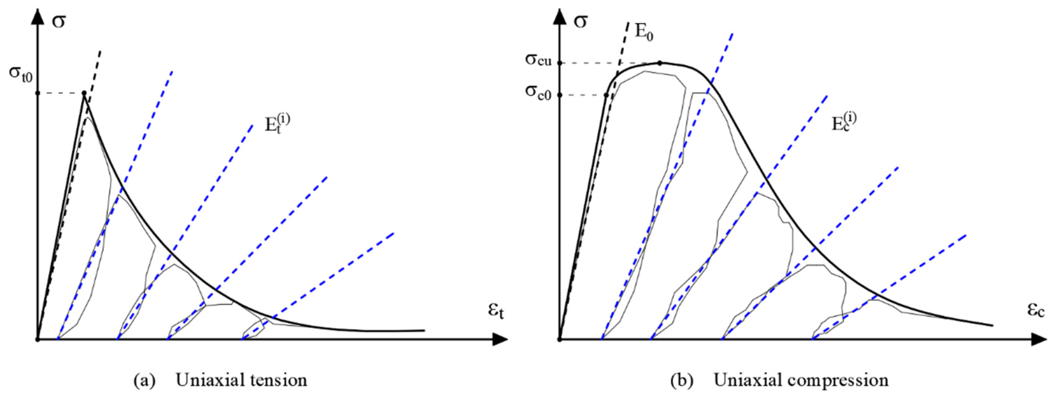
3.2.4. Concrete Damaged Plasticity Failure Criterion (CDP)

The Concrete Damaged Plasticity Model (CDP) is a criterion that was created for frictional materials, rocks and therefore for almost fragile materials such as concrete as an evolution of the Mohr-Coulomb and Drucker-Prager criteria, from which it takes the basis for the definition of the yield function [1]. The latter together with the flow rule and the hardening rule, represent the fundamental elements for the definition of a plasticity model. In the specific case, the innovative aspect lies in replacing the hardening variable with a plastic-damage variable (k), always increasing like the previous one (stability) and directly proportional to the plastic deformation ${\epsilon }_p$. The plastic-damage variable, dimensionless, can assume values between 0 and 1 which correspond to the limit cases of zero-damage and total damage, associated with the formation of macroscopic fractures. The damage is applied to the cohesion c which will no longer be a constant parameter as in the case of the Mohr-Coulomb and Drucker-Prager criteria but will depend on the value assumed by the plastic-damage variable. The value of the cohesion c will initially be equal to $f_0$, that is the uniaxial yield stress (compression-traction), which corresponds to a damage function $k=0$ while it will be equal to 0 if $k=1$ (total damage). In this way, it will be possible to follow the evolution of the yield surface as the plastic deformation varies [10,11,12].

The damage parameter can be defined starting from the uniaxial stress states in traction and compression. Assuming to have the experimental stress-strain diagrams and converting them into plastic stress-strain diagrams $\sigma -{\epsilon }_p$ (Figure 10).

For the traction it is defined:

$$k_t=\frac{1}{g_t}{{\displaystyle \int }}_0^{{\epsilon }_p}\sigma d{\epsilon }_p$$

(50)

with $g_t$ equal to the area under the curve in traction. By setting $k_t$ as an independent variable, it is possible to express the tension according to a function of the type $\sigma =f_t\left(k_t\right)$, respecting the conditions $f_t\left(0\right)=f_{t_0}$ and $f_t\left(1\right)=0$, with $f_{t_0}$ yield strength in traction. Similarly, for compression we can write:

$$k_c=\frac{1}{g_c}{{\displaystyle \int }}_0^{{\epsilon }_p}\sigma d{\epsilon }_p$$

(51)

with $g_c$ equal to the area under the curve in traction. By setting $k_c$ as an independent variable, it is possible to express the tension according to a function of the type $\sigma =f_t\left(k_t\right)$, fulfilling the conditions $f_t\left(0\right)=f_{t_0}$ and $f_t\left(1\right)=0$, with $f_{c_0}$ yield strength in compression.

A possible function $f\left(k\right)$ compatible with the experimentally observed behaviour with asymptotic tendency to zero in terms of tension is the following (valid for both the branches of Figure 10):

$$\sigma =f_0\left[\left(1+a\right)\exp \left(-b{\epsilon }_p\right)-a exp\left(-2b{\epsilon }_p\right)\right]$$

(52)

where a e b are constant if the function $g={\int }_0^{\infty }\sigma d{\epsilon }_p$, that is, the area underlying the function that defines the $\sigma -{\epsilon }_p$ link and its derivative $d\sigma /d{\epsilon }_p$ for ${\epsilon }_p=0$, are provided according to the relationships:

$$g=\frac{f_0}{b}=\left(1+\frac{a}{2}\right)$$

(53)

$${\frac{d\sigma }{d{\epsilon }_p}|}_{{\epsilon }_p=0}=f_{0}b\left(a-1\right)$$

(54)

A value of $a>1$ implies an initial hardening phase, whereas a value of $a<1$ implies a softening branch after yielding. From the integration of Equations (50) and (51), considering (52), we obtain a final expression of the damage parameter $k\left({\epsilon }_p\right)$ as a function of the plastic deformation.

The extension of the previous definitions to the case of pluriaxial tension is provided in differential terms starting from the cases of biaxial compression and traction, according to the following relationships:

$$\dot{k_t}=\frac{1}{g_t}{f}_t\left(k\right){\dot{\epsilon }}_1^p$$

(55)

$$\dot{k_c}=-\frac{1}{g_c}{f}_c\left(k\right){\dot{\epsilon }}_3^p$$

(56)

A more general formulation, valid for any state of tension that is neither pure tension nor pure compression (for instance ${\sigma }_1>0, {\sigma }_3<0$) can be expressed according to the following relationship:

$$\dot{k}=\frac{r\left(\sigma \right)}{g_t}{f}_t\left(k\right){\dot{\epsilon }}_1^p-\frac{1-r\left(\sigma \right)}{g_c}{f}_c\left(k\right){\dot{\epsilon }}_3^p$$

(57)

where $r\left(\sigma \right)$ is a factor included between 0 e 1. For $r\left(\sigma \right)=1$, the tensions are ${\sigma }_i>0$ for each $i, i=1,2,3$ and Equation (57) is coincident with Equation (55), for biaxial traction. For $r\left(\sigma \right)=1$, the tensions ${\sigma }_i>0$ for each $i, i=1,2,3$ and Equation (57) is coincident with Equation (56), which is the case of biaxial compression. The parameter $r\left(\sigma \right)$ can be expressed in the following form:

$$r\left(\sigma \right)=\frac{{\sum }_{i=1}^3\langle {\sigma }_i\rangle }{{\sum }_{i=1}^3\left|{\sigma }_i\right|}$$

(58)

where (the Macauley bracket) $\langle x\rangle =\frac{1}{2}\left(\left|x\right|+x\right)$.

The yield function starts from the extended Drucker-Prager formulation, replacing the dependence on the third invariant of the $J_3$ deviatoric stress tensor with the algebraically largest principal stress. This term provides greater adherence in the representation of differences in behaviour in the tension and compression regions. The function can be expressed as follows:

$$f\left(I_1,J_2,{\sigma }_{max}\right)=\frac{1}{1-\alpha }\left[\sqrt{3J_2}+\alpha I_1+\beta \langle {\sigma }_{max}\rangle -\gamma \langle {\sigma }_{max}\rangle \right]-c_0=0$$

(59)

where $\alpha ,\beta ,\gamma$ must be provided experimentally. For ${\sigma }_{max}=0$, namely in the case of biaxial compression, the criterion essentially takes the form of Drucker-Prager, and the biaxial tension can be expressed in the following way (the tensions are reported with their own sign):

$$f\left(I_1,J_2,{\sigma }_{max}=0\right)=\frac{1}{1-\alpha }\left[\sqrt{f_{b_0}{}^2}-2\alpha f_{b_0}\right]-f_{c_0}=0$$

(60)

By considering the initial cohesion equal to $f_{c_0}$ and the initial equibiaxial compressive stress $f_{b_0}$, it is possible to write [14,15]:

$$\frac{f_{b_0}}{f_{c_0}}=\frac{1-\alpha }{1-2\alpha }$$

(61)

and as a consequence:

$$\alpha =\frac{\left(f_{b_0}/f_{c_0}\right)-1}{2\left(f_{b_0}/f_{c_0}\right)-1}$$

(62)

Experimentally, the ratio reported in Equation (61) evidenced a value included between 1.10 and 1.16, and therefore the value of $\alpha$ is included between 0.08 and 0.12. In case of uniaxial tension:

$$f\left(I_1,J_2,{\sigma }_{max}=f_{t_0}\right)=\frac{1}{1-\alpha }\left[\sqrt{f_{t_0}{}^2}+\alpha f_{t_0}+\beta f_{t_0}\right]-f_{c_0}=0$$

(63)

And:

$$\frac{f_{c_0}}{f_{t_0}}=\frac{1+\alpha +\beta }{1-\alpha }$$

(64)

$$\beta =\left(1-\alpha \right)\left( f_{c_0}/f_{t_0}\right)-\left(1+\alpha \right)$$

(65)

The parameter $\gamma$ is present only in case of triaxial compression. In order to evaluate it, we can exploit the TM (tensile meridian) for which it results that ${\sigma }_1>{\sigma }_2={\sigma }_3; \theta =0°$ and CM (compressive meridian) for which it results that ${\sigma }_1={\sigma }_2>{\sigma }_3; \theta =60°$. By Equation (14) which allows to express the principal stresses as a function of the invariants $I_1,J_2$ and of the angle in the deviatoric plane $\theta$, it can be written for the first case:

$${\sigma }_{max}=\frac{1}{3}\left(I_1+2\sqrt{3J_2}\right)=0$$

(66)

and for the second case:

$${\sigma }_{max}=\frac{1}{3}\left(I_1+\sqrt{3J_2}\right)=0$$

(67)

The expressions of the respective meridians can be written as follows:

$$\left(2\gamma +3\right)\sqrt{3J_2}+\left(\gamma +3\alpha \right)I_1=\left(1-\alpha \right)f_c$$

(68)

$$\left(\gamma +3\right)\sqrt{3J_2}+\left(\gamma +3\alpha \right)I_1=\left(1-\alpha \right)f_c$$

(69)

where $f_c$ is the critical stress in uniaxial compression, defined as yield stress or ultimate stress depending on the location in the domain (yield surface or Failure surface). By defining $\tilde{\rho }$ the ratio between the meridians TM and CM (Figure 11), it is possible to write:

$$\stackrel{\sim }{\rho } =\frac{\gamma +3}{2\gamma +3}$$

(70)

and

$$\gamma =\frac{3\left(1-\rho \right)}{2\rho -1}$$

(71)

The constants $\alpha ,\beta ,\gamma$ as the coesion $c_0=f_{c_0}$, through the function $f_c\left(k\right)$ and $f_t\left(k\right)$ change their value and determine the evolution of the failure domain as a function of the level of damage reached.

As for the flow rule, it is non-associative to control the high plastic expansion that characterizes the frictional materials. Lubliner [15] proposes to use the Mohr-Coulomb yield function as a potential function $G$ by replacing the internal friction angle $\phi$ with the dilation angle $\Psi$:

$$G(I_1,J_2,\Psi )=\frac{I_1}{3}sin\Psi +\sqrt{J_2}\left(cos\theta -\frac{sin\theta sin\Psi }{\sqrt{3}}\right)$$

(72)

Alternatively, Lee in 1998 proposes the Drucker-Prager yield function as Flow potential function G (Equation (38)) [16,17,18,19].

The damage function can also be applied to consider the variation of the elastic modulus $E_0$ as the plastic deformation ${\epsilon }_p$ increases. In terms of tensions, it can be written:

$$\sigma =\left(1-k\right)E_0 \left(\epsilon -{\epsilon }_p\right)$$

(73)

which became for the elastic modulus E in the following function:

$$E=\left(1-k\right)E_0$$

(74)

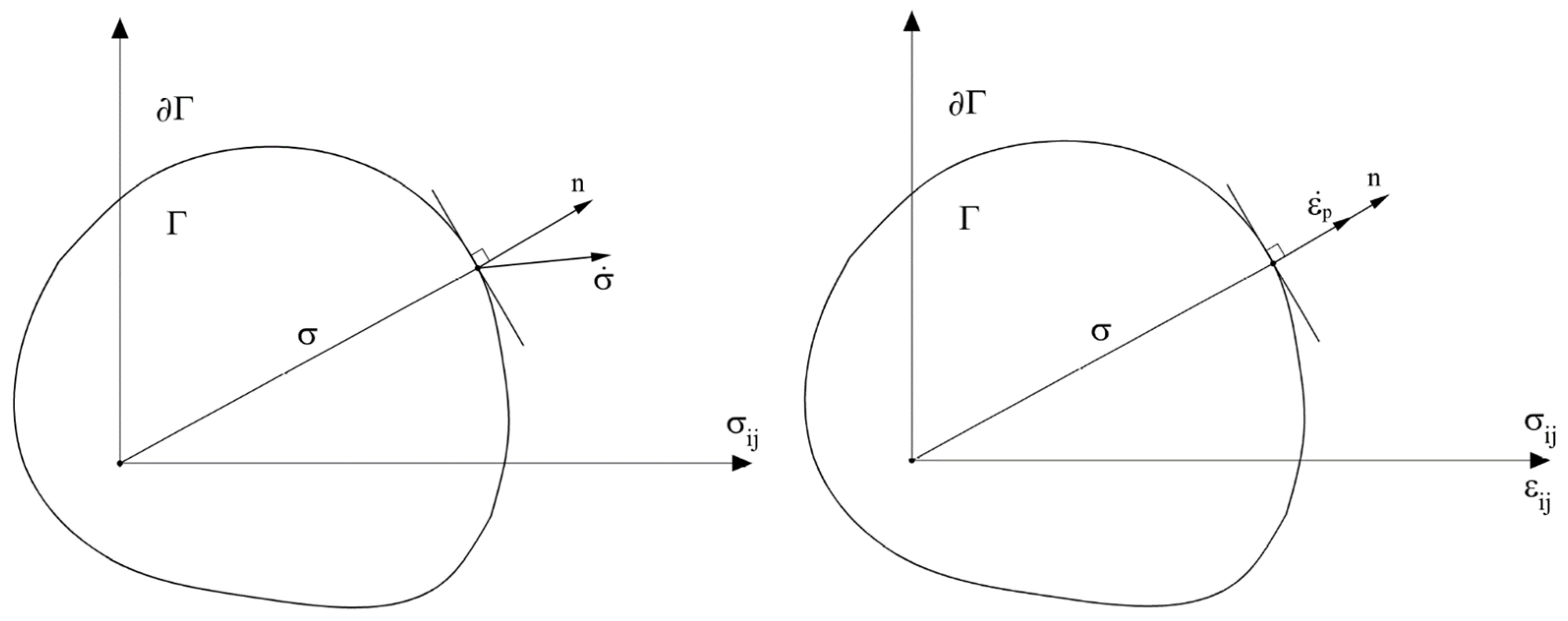
3.3. Yield Function, Flow Rule and Hardening Rule

The bases of classical plasticity theory, in addition to the yield function, are the flow rule and the hardening rule which allow, through the incremental stress-strain link, to define the evolution of the failure surface and therefore of the plasticity condition itself. By operating in the space of the components of the stress tensor, it is possible to obtain a clear interpretation of the Equations (75) and (76). Graphically, the function $f\left(\underset{\_}{\sigma }\right)=0$ represents a limit boundary, a hypersurface $\partial \Gamma$, while the stress state is represented by a point or in any case by a vector, whose components in the reference system assumed are precisely the stresses ${\sigma }_{ij}$. Having defined the plasticity function $f\left(\underset{\_}{\sigma }\left(\underset{\_}{X}\right)\right)$, dependent on the state of point stress (Equation (15)), it is possible to state that the behaviour is not plastic if:

$$\{\begin{array}{c}f\left(\underset{\_}{\sigma }\right)<0\\ or f\left(\underset{\_}{\sigma }\right)=0 ; {\left(\frac{\partial f}{\partial \underset{\_}{\sigma }}\right)}^T·\underset{\_}{\dot{\sigma }}<0 \end{array}$$

(75)

while it is plastic when:

$$f\left(\underset{\_}{\sigma }\right)=0 ; {\left(\frac{\partial f}{\partial \underset{\_}{\sigma }}\right)}^T·\underset{\_}{\dot{\sigma }} \ge 0$$

(76)

The variation of the tensional state $d{\sigma }_{ij}$ are defined through the temporal derivative of the tension vector $\underset{\_}{\dot{\sigma }}$ which provides in terms of components $\dot{{\sigma }_{ij}}=\frac{d{\sigma }_{ij}}{dt}$. The ratio $\frac{\partial f}{\partial \underset{\_}{\sigma }}$ is the gradient of the plasticity function $\underset{\_}{\nabla f}$ which is the vector normal to the surface of components $\frac{\partial f}{\partial {\sigma }_{ij}}$. Therefore, it is possible to write:

$${\left(\frac{\partial f}{\partial \underset{\_}{\sigma }}\right)}^T·\underset{\_}{\dot{\sigma }}={\underset{\_}{n}}^T·\underset{\_}{\dot{\sigma }}$$

(77)

The sign of the scalar product in Equation (77) allows checking the evolution of the tensional state for a point lying on the boundary of the domain. For ${\underset{\_}{n}}^T·\underset{\_}{\dot{\sigma }}<0$, the vector $\underset{\_}{\dot{\sigma }}$ is oriented inwards (non-holonomy at unloading-elastic behaviour), while, for ${\underset{\_}{n}}^T·\underset{\_}{\dot{\sigma }}>0$ the vector is oriented outwards (plastic behaviour). If ${\underset{\_}{n}}^T·\underset{\_}{\dot{\sigma }}=0$ we have a pure plastic behaviour with a vector $\underset{\_}{\dot{\sigma }}$ tangent to $\partial \Gamma$.

3.3.1. Flow Rule

Once the plasticity condition has been defined, it is necessary to obtain a law that allows deriving the plastic deformations. One possibility is represented by the direct proportionality between the plastic deformation rate ${\dot{\epsilon }}_{ij}^p$ and the homologous component of the gradient of a function g(σ), called the flow function:

$${\dot{\epsilon }}_{ij}^p=\dot{\lambda }\frac{\partial g}{\partial {\sigma }_{ij}}$$

(78)

where $\dot{\lambda }$ is an unknown scalar function that assumes values other than zero only in the occurrence of plastic deformation. When $f=g$, i.e., when the plasticity function is coincident with the flow function Equation (12) can be rearranged as:

$${\dot{\epsilon }}_{ij}^p=\dot{\lambda }\frac{\partial f}{\partial {\sigma }_{ij}}$$

(79)

In this case, the flow rule is associated because the plastic flow is related to the yielding surface, conversely, when $f\ne g$ the flow rule is non-associated.

From the geometric point of view, by superimposing on the reference system with axes represented by the components of the stress ${\sigma }_{ij}$ a system that supports the components of the plastic deformation rate ${\dot{\epsilon }}_{ij}^p$, it is possible to make some considerations. In the case $f=g$, the vector $\underset{\_}{\dot{{\epsilon }^p}}$, through the function $f$, has the same direction and sense as the normal to the surface n (Figure 12). For the properties highlighted, Equation (79) is known as the law of normality. This law leaves indeterminate the factor $\dot{\lambda }$ and the modulus of the vector $\underset{\_}{\dot{{\epsilon }^p}}$ indicative of the amplitude of the plastic deformations.

3.3.2. Drucker Stability Postulate

Drucker’s postulate completes the theory of plastic potential. Drucker states that if a material is stable there is a potential function and it coincides with the plasticity function, which must be a convex surface in the space of stresses. Compared to a uniaxial experimental test, a material is defined as stable if any monotonic variation of the tension $d\sigma$ is accompanied by a variation of the same sign of $\epsilon$. In the case of perfectly plastic behavior, the stability is defined as neutral. In a general way a material can be defined stable if, given a stress state, the work due to additional external forces, independent from the original ones, for a complete loading-unloading cycle, is not negative.

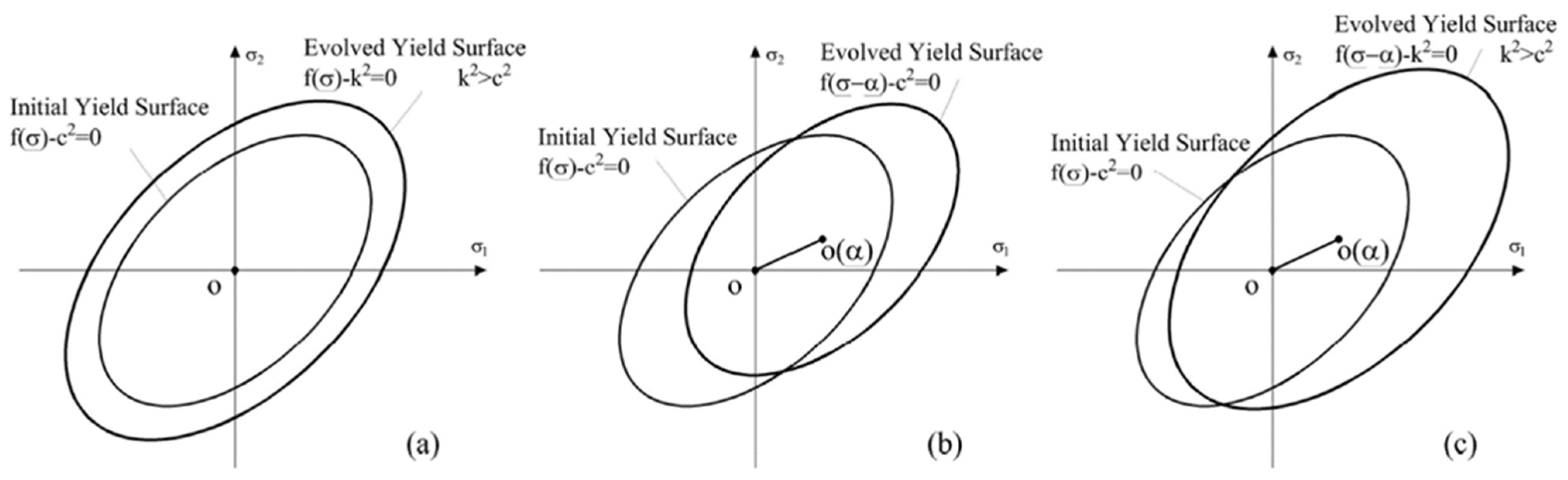
3.3.3. Hardening Rule

The last aspect that completes the theory of classical plasticity is the hardening rule. Remaining within the scope of Drucker’s postulate, it is possible to define hardening with a function as $f=f\left(\underset{\_}{\sigma },k, {\underset{\_}{\epsilon }}^p\right)$, in which the plastic work $k={\underset{\_}{\sigma }}^T·{\underset{\_}{\epsilon }}^p$ and the plastic deformations ${\underset{\_}{\epsilon }}^p$ are parameters suitable for reconstructing the history of plastic deformations. The condition of congruence, that is the condition of belonging of the final (increased) tension point to the evolved plastic surface is:

$$\dot{f}={\left(\frac{\partial f}{\partial \underset{\_}{\sigma }}\right)}^T·\underset{\_}{\dot{\sigma }}+\frac{\partial f}{\partial k}\dot{k}+{\left(\frac{\partial f}{\partial {\underset{\_}{\epsilon }}^p}\right)}^T·{\underset{\_}{\dot{\epsilon }}}^p=0$$

(80)

Keeping in mind the normality condition (Equation (79)), valid only for associative plasticity, and that $\dot{k}={\underset{\_}{\sigma }}^T·{\dot{\underset{\_}{\epsilon }}}^p={\underset{\_}{\sigma }}^T·\dot{\lambda }\frac{\partial f}{\partial \underset{\_}{\sigma }}$ and $\partial f/\partial \underset{\_}{\sigma }=\underset{\_}{n}$, the condition of congruence (Equation (80)) can be rearranged as:

$${\underset{\_}{n}}^T·\underset{\_}{\dot{\sigma }}-h\dot{\lambda }=0$$

(81)

where $h$ is called the work hardening function. From Equation (81) it is evident that in the context of plastic deformations for a stable material ($\dot{\lambda } >0$), it is necessary that $h>0$ or for a neutral material $h=0$. In cases where $h>0$, it is possible to define simple hardening rules that govern approximately the evolution of the plasticity domain and therefore the development of plastic deformations. In particular, it is possible to define (Figure 13):

• Isotropic hardening: this is the simplest hardening rule and is based on the concept of homothetic expansion of the initial yield surface, without any kind of distortion or translation. The function is characterized by a single parameter k and takes the form:

$$f=f\left(\underset{\_}{\sigma }\right)-k^2$$

(82)

• Kinematic hardening: in this case the surface translates into the space of tensions, keeping its shape, orientation and size rigid unchanged. The evolved domain is characterized by a variable center as a function of the plastic deformations:

  $$f=f\left(\underset{\_}{\sigma }-\underset{\_}{\alpha }\right)-c^2$$

  (83)

  with c constant and $\underset{\_}{\alpha }$ defined through the Prager or Ziegler rule which determines these parameters as a function of the history of plastic deformation.

• Combined hardening: isotropic hardening is accepted in the case of proportional increasing actions; kinematic hardening is used when the Bauschinger effect prevails. In many cases, the behaviour turns out to be mixed and for this reason, a work hardening function has been defined that contemplates both the previously exposed types and can be written as:

$$f=f\left(\underset{\_}{\sigma }-\underset{\_}{\alpha }\right)-k^2\left({\underset{\_}{\epsilon }}^p\right)$$

(84)

3.3.4. Non-Associated Flow Rule

The condition of normality from which the concept of associated flow rule arises, convexity, uniqueness, and continuity, are consequences of Drucker’s stability postulate. It is right to point out, however, that the conditions it poses are sufficient but not necessary. If the uniqueness of the solution is verified, the material must be locally stable. For geomaterials, cement and even masonry, it has been proven that the associative flow rule tends not to provide a correct estimate of the plastic volumetric expansion (Figure 14). For this type of material, the volume variation during hardening is characterized by a contraction at the beginning of the yielding phases and by a volumetric expansion which is expressed in its entirety only around 75–90% of the ultimate load. This behaviour is often violated by the associated flow rule. A parameter that allows you to control the volumetric expansion is the dilation angle 𝛹 used as an alternative to the friction angle $\phi$ in the case of the Mohr-Coulomb and Drucker-Prager failure criteria. In particular, it is considered a non-associative flow rule if $\Psi \ne \phi$.

The dilation angle is generally determined through triaxial tests or direct shear tests, and it assumes different values according to the considered material. The values of $\Psi$, as suggested by Vermeer and De Borst in 1984, start from 0° for normally consolidated clay, passing through concrete with 12° up to 20° for compact marbles. Particular types of masonry can have dilation angles of up to 30° [6,15,16].

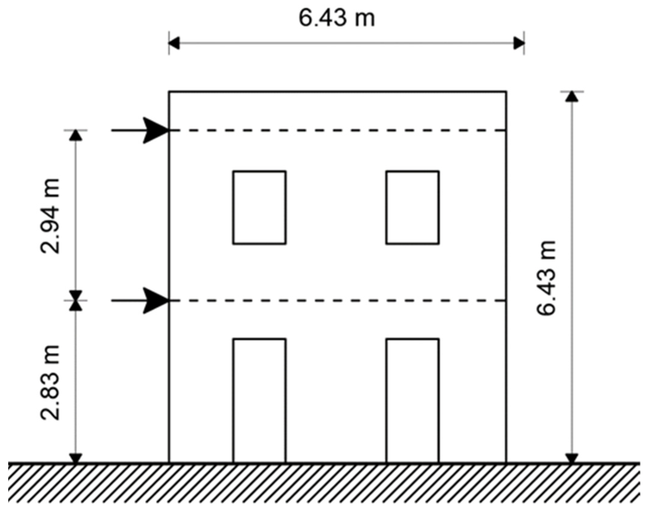
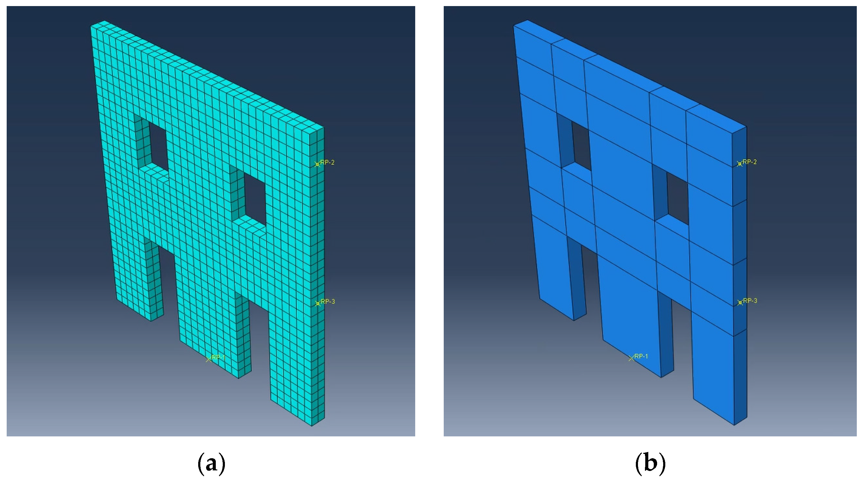
4. Case Study: Application to a Masonry Wall

To evaluate and motivate the choice of a specific macromechanical failure criterion for masonry buildings, the so-called Pavia Door Wall experimental tests have been selected from the literature because of the availability of wide information and data [10]. The reference building is a two-storey building, in ordinary masonry, with rigid floors, for which a total of seven configurations have been considered, varying according to the arrangement of the openings on the four sides and any elements resistant to traction, coupled to the floor strips. The configurations examined, called “door wall”, was tested at the University of Pavia in 1994, as part of a test pseudo-static cyclic test [12,13].

During the test, the building was subjected to cyclic displacements at the level of the rigid decks, in order to obtain a distribution of forces proportional to the seismic weights.

The plan size is 4.40 × 6.00 m, while the total height is 6.43 m. The height of the first deck is 2.83 m, while the second is 2.94 m from the first, the wall thickness is 0.25 m. The applied overloads are 248.8 kN at the first level and 236.8 kN at the second. The comparisons were made with reference to the study on the non-linear static analysis of masonry walls [10,11,12] which re-proposes the results of incremental static analysis from different modelling, applied to the “Door Wall of Pavia” (Figure 15). In

Table 1. Mechanical parameters of the Pavia Door Wall.

	E [MPa]	G [MPa]	fwc [MPa]	fvd0 [MPa]	c [MPa]	μ [−]	fbt [MPa]
Masonry	1400	480	6.20	0.18
Mortar					0.23	0.58
Bricks							1.22

, the mechanical properties of the ordinary brick masonry of the Pavia Door Wall building, used, below, for the calibration carried out in this work using the ABAQUS software, are reported. In particular, E is the Young modulus, G is the tangential modulus, f_wc is the masonry compressive strength, f_vd0 is the shear resistance in absence of the axial load, c is the mortar cohesion, μ is the friction coefficient and f_bt is the tensile resistance of masonry blocks.

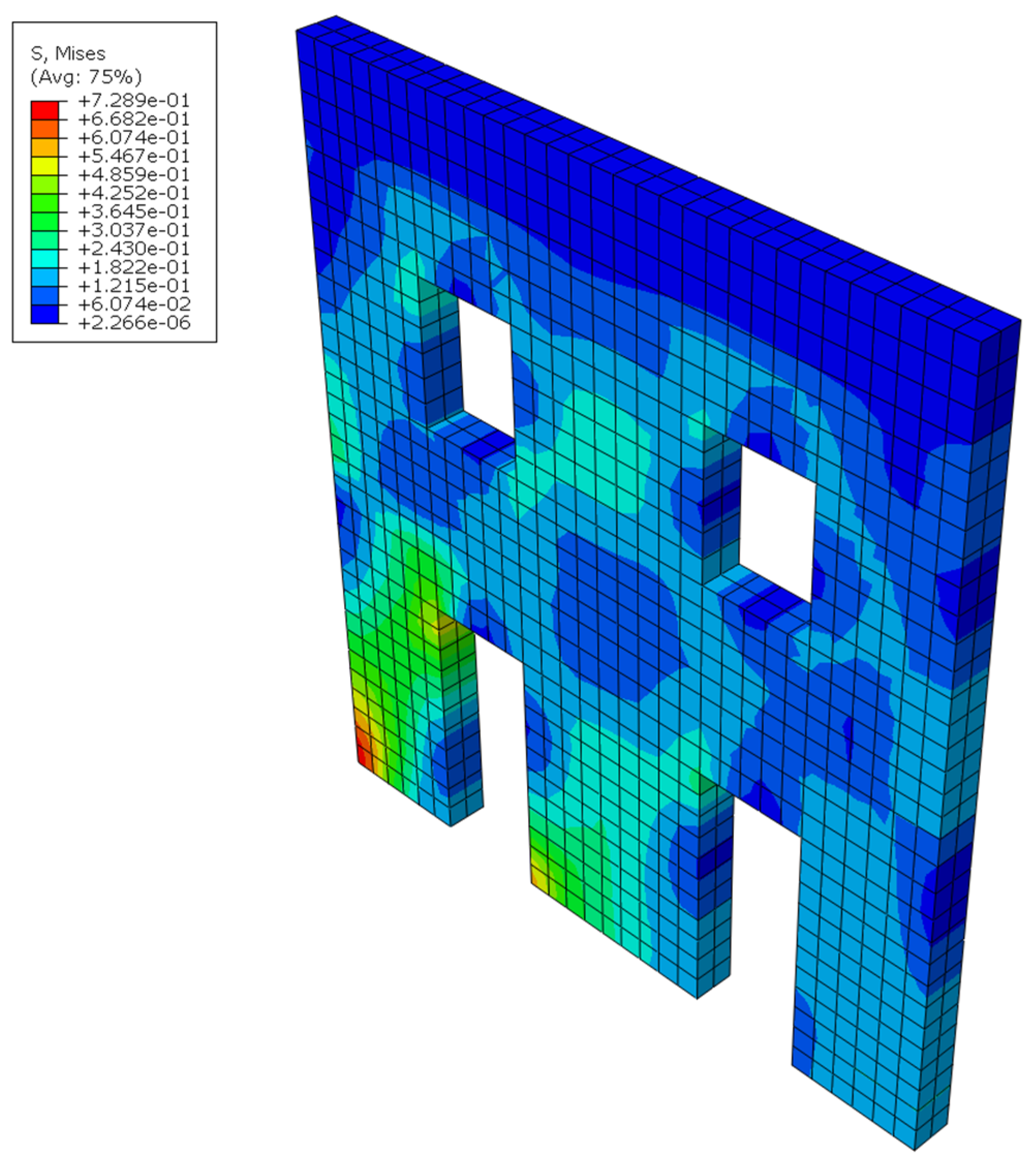
4.1. FEM Model and Numerical Analysis

The Pavia “Door Wall” of was modelled, in Abaqus without scaling, and with the real applied loads, simulating the test carried out experimentally. The analysis is carried out first on a solid, three-dimensional model with linear hex meshes with reduced integration (C3D8R) with the size of about 100 mm (see Figure 16a). The partitioning procedure (see Figure 16b) has the aim of regularize the mesh. In particular, the partitions are made by identifying the characteristic elements that make up the masonry, that is, the nodal areas, the masonry walls and the floor strips. The couplings are created in correspondence with the two rigid decks and the attachment section at the base. This type of constraint ensures that all selected points, at the same elevation, move in the same way. A reference point is subsequently chosen for each coupling, to which boundary conditions are applied. A displacement boundary condition is applied to the height of the two rigid decks, allowing the displacement only in the horizontal direction $x$; at the base, an encastre is placed to avoid displacements or rotations in any direction.

The numerical model is loaded with distributed actions, horizontal forces consistent with the distribution of the masses and the self-weight. Non-linear analysis was performed using an explicit dynamic procedure, implemented in a quasi-static manner. This type of analysis allows the use of damage parameters in compression and tension, given through a table curve, according to the theory of large deformations. Consequently, the explicit analysis is highly effective for the study of damage and degradation of masonry structures, including cracks it is possible to trace very carefully the propagation of damage that occurs gradually (such as cracking and crushing) under an increasing load value, regardless of the type of load. The ABAQUS package offers several other methods that perform dynamic analysis of nonlinear problems, such as implicit dynamic analysis. However, implicit dynamic analysis is not as effective as the explicit approach. The experience [17,18,19,20,21] shows that in the modelling of complex non-linear problems, such as damage to masonry structures, convergence problems often emerge at the beginning of structural degradation. A disadvantage of explicitly dynamic analysis is the sensitivity to very small elements that force the entire model to be integrated with a small increase in time. Variable integration steps or subcycling methods can be used to fix this problem.

Authors thank the reviewer for the comment. According to the reviewer suggestion the following sentences have been added in the FEM simulation chapter:

The sensitivity analysis was performed by varying the competent parameters of the model and the chosen failure criterion, analyzing the possible correlation between them. The procedure was performed through the following criteria:

Firstly, the base case output is defined; the input value (V1) for which the sensitivity has to be measured is selected. All the other inputs of the model are kept constant.

Then the value of the output at a new value of the input (V2) is calculated, keeping the other inputs as constant.

The percentage scatter in the input and output are evaluated.

The sensitivity is calculated by dividing the percentage scatter in output by the per-centage in input.

Referring to the concrete damaged plasticity, from the sensitivity analysis it was noted that the variation of the parameters adopted for the characterization of the flow Rule (Ψ, ε, K) influence the result not as significantly as the parameters that govern the curves of uniaxial tension and uniaxial compression (These parameters are 5 times more relevant). Consequently, to obtain reliable results it is necessary to have models capable of adequately representing the experimental curve of the material considered, in traction and compression. Guo’s model proved to be easy to use and widely adaptable in the calibration process.

4.2. Extended Drucker-Prager

Among the models implemented within the Abaqus software, the Drucker—Prager model, or rather, its extension, has the characteristic of including the dependence of the failure surface on the third invariant of the deviatoric stresses J₃. For this model, three types of yield criteria are available in the software: linear, hyperbolic, and exponential. The linear model provides a non-circular section on the deviatoric plane which allows more precise calibration of the model for the Mohr-Coulomb parameters. The hyperbolic and exponential models, on the other hand, use a Von Mises section, therefore circular, in the deviatoric plane. The choice of the type of model depends on the type of analysis, the type of material, and above all also on the experimental data available for the calibration of the model parameters. In general, the hyperbolic model is suitable for brittle materials for which data from both triaxial compression and triaxial tension tests are available. The exponential model is the most general of the three and determines the parameters starting from the data deriving from the triaxial tests.

The linear model, on the other hand, can be used in the case in which experimental data already calibrated in terms of cohesion and friction angle, similar to the Mohr-Coulomb criterion, are available. In the specific case, reference is made to the linear model. This is written about the invariants $I_1, J_2, J_3$ and is formulated as:

$$f=t-p tan\beta -c=0$$

(85)

where:

$$p=-\frac{I_1}{3}$$

(86)

$$q=\sqrt{\frac{3}{2}\left(\stackrel{=}{T^{\prime }}:\stackrel{=}{T^{\prime }}\right)}=\sqrt{3J_2}$$

(87)

$$r={\left[\frac{9}{2}\left(\stackrel{=}{T^{\prime }}:\stackrel{=}{T^{\prime }}:\stackrel{=}{T^{\prime }}\right)\right]}^{\frac{1}{3}}={\left(\frac{27}{2}{J}_3\right)}^{\frac{1}{3}}$$

(88)

$$t=\frac{1}{2}q\left[1+\frac{1}{K}-\left(1-\frac{1}{K}\right){\left(\frac{r}{q}\right)}^3\right]$$

(89)

$c$ is the material cohesion parameter, $\beta$ is the internal friction angle and K is the flow stress ratio, i.e., the ratio of the meridians in compression ${\rho }_{c_0}$ and traction ${\rho }_{t_0}$ for 𝜉 = 0. The K parameter must be included in the range $0.778\le K\le 1$ so that the fracture surface remains convex. For $K=1, t=q$ the deviatoric section coincides with the Von Mises circle. The parameter of cohesion $d$ is computed in ABAQUS through its correlation with the uniaxial tensional states. If the hardening is defined by the cohesion we have:

$$c=c$$

(90)

while, if the hardening is uniaxial in compression it becomes:

$$c=\left(1-\frac{1}{3}tan\beta \right){\sigma }_c$$

(91)

and in tension:

$$c=\left(\frac{1}{K}+\frac{1}{3}tan\beta \right){\sigma }_t$$

(92)

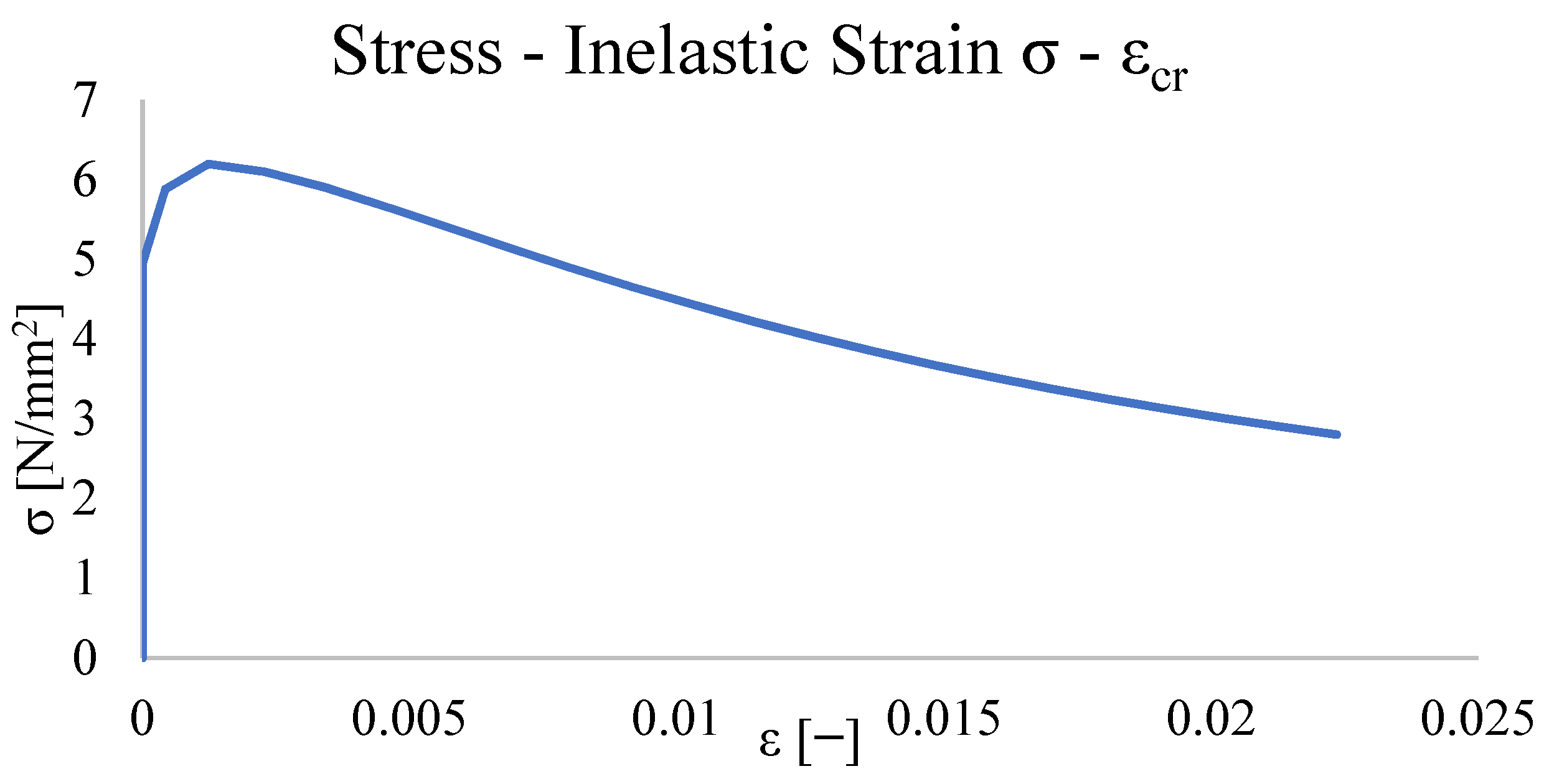
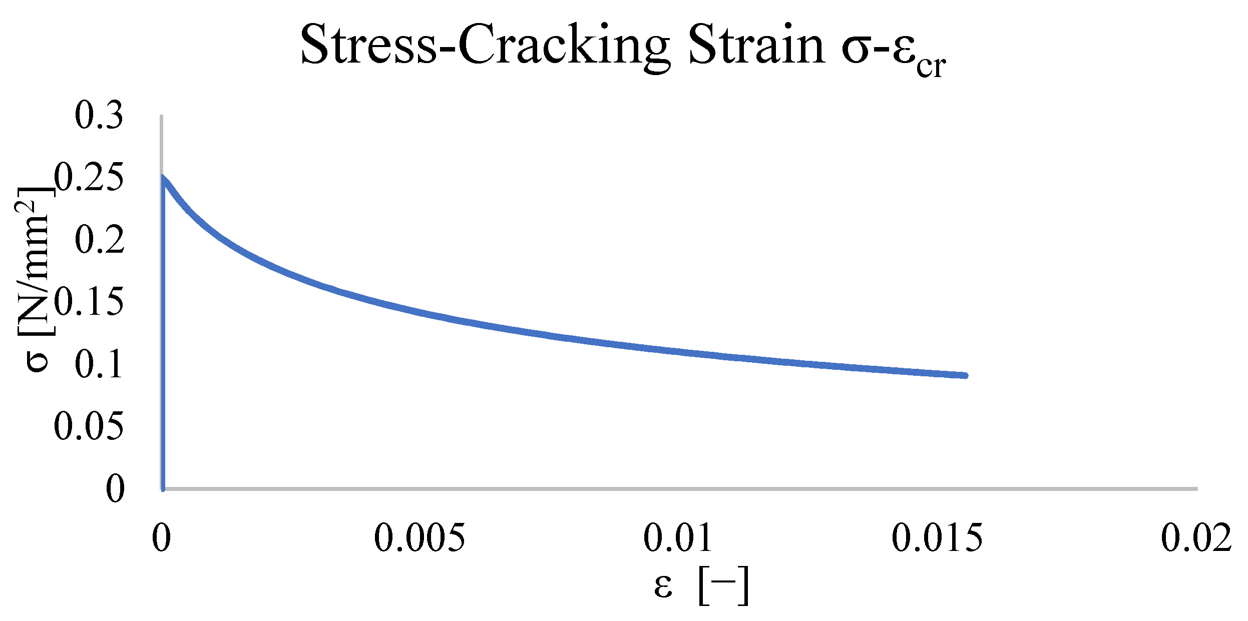
4.3. Concrete Damaged Plasticity

The Concrete Damaged Plasticity is a continuous model based on two main failure mechanisms, namely the tensile cracking and compressive crushing.

The evolution of the damage and therefore of the failure surface is governed by two variables, namely ${\epsilon }_t^p$ and ${\epsilon }_c^p$, respectively representative of the plastic deformation in traction and compression [13,15,17]. These variables are associated with the possible mechanisms of rupture in tension and compression (Figure 17). By defining $d_t$ and $d_c$ the tensile and compressive damage functions, respectively, the stress-strain relations can be rewritten as follows:

$${\sigma }_t=\left(1-d_t\right)E_0\left({\epsilon }_t-{\epsilon }_t^p\right)$$

(93)

$${\sigma }_c=\left(1-d_c\right)E_0\left({\epsilon }_c-{\epsilon }_c^p\right)$$

(94)

with $d_t$ and $d_c$ equal to 0 in case of zero damage and equal to 1 in case of total damage. The reduced elastic modulus E is represented by $E=\left(1-d_t\right)E_0$ in tension and $E=\left(1-d_c\right)E_0$ in compression.

In the case of uniaxial cyclic loading, the opening and closing of the micro-cracks and their interaction play a fundamental role. Experimentally it has been shown that there is a recovery of elastic stiffness in the moment of inversion of the stress sign and it is greater in the case of transition from tension to compression. In this case, for the reduction of the elastic modulus, reference is made to a single damage variable d which will be a function of the previously described damage parameters $d_t$ and $d_c$, of the scalar functions $s_t$ and $s_c$, dependent on the stress state and which allow to particularize the relation as a function of the passage from positive to negative stresses or vice versa and finally of the weight factors $w_t$ and $w_c$, which represent the extent of the recovery of stiffness in the compression-tension and tension-compression passage (Figure 18).

The elastic modulus E can be expressed by the following relationship:

$$E=\left(1-d\right)E_0$$

(95)

The reduction factor $\left(1-d\right)$, is valid for both tension (${\sigma }_{11}>0)$ and compression ${\sigma }_{11}<0$ and it can be furtherly written as:

$$\left(1-d\right)=\left(1-s_t{d}_c\right)\left(1-s_c{d}_t\right)$$

(96)

where the stress reversal functions $s_t$ and $s_c$ are:

$$s_t=1-w_t{r}^{*}\left({\sigma }_{11}\right); 0\le w_t\le 1$$

(97)

$$s_c=1-w_c\left(1-r^{*}\left({\sigma }_{11}\right)\right); 0\le w_c\le 1$$

(98)

where $r^{*}$ is a step function dependent on the sign of the stresses:

$$r^{*}\left({\sigma }_{11}\right)=\{\begin{array}{c}1 if {\sigma }_{11}>0 \\ 0 if {\sigma }_{11}<0 \end{array}$$

(99)

In pluriaxial cases the previously exposed relationships are generalized by replacing the step function $r^{*}\left({\sigma }_{11}\right)$ with the pluriaxial weight factor $r\left(\sigma \right)$ (Equation (58)) and applied to the initial elasticity matrix $\stackrel{=}{D_0}$ according to the relationship:

$$\left(1-d\right)\stackrel{=}{D_0}\left(\underset{\_}{\epsilon }-\underset{\_}{{\epsilon }_p}\right)$$

(100)

The ABAQUS software foresees the definition of the uniaxial behaviour in tension as a function of the cracking strain ${\epsilon }_t^{ck}$, defined as the difference between the total deformation and the elastic deformation corresponding to a material without damage ($d_t=0$). In analytical terms it results:

$${\epsilon }_t^{ck}={\epsilon }_t-{\epsilon }_{0t}^{el}$$

(101)

with ${\epsilon }_{0t}^{el}={\sigma }_t/E_0$.

The software subsequently converts the cracking strain into plastic strain according to the relationship:

$${\epsilon }_t^p={\epsilon }_t^{ck}-\frac{d_t}{\left(1-d_t\right)}\frac{{\sigma }_t}{E_0}$$

(102)

Regarding the uniaxial behaviour in compression, ABAQUS foresees the use of data as a function of the inelastic strain ${\epsilon }_c^{in}$, defined as the difference between the total deformation and the elastic deformation corresponding to material without damage ($d_t=0$). In analytical terms, it results:

$${\epsilon }_c^{in}={\epsilon }_c-{\epsilon }_{0c}^{el}$$

(103)

with ${\epsilon }_{0t}^{el}={\sigma }_t/E_0$.

The software subsequently converts the inelastic strain into plastic strain according to the relationship:

$${\epsilon }_c^p={\epsilon }_c^{in}-\frac{d_c}{\left(1-d_c\right)}\frac{{\sigma }_c}{E_0}$$

(104)

The data ${\sigma }_t-{\epsilon }_t^{ck}$ and ${\sigma }_c-{\epsilon }_c^{in}$ must be implemented in the software by tables. The damage parameters $d_t$ and $d_c$, must be reported with the same intervals of ${\epsilon }_t^{ck},{\epsilon }_c^{in}$ provided for the tensions.

The yielding or failure function $f$ is provided according to Equation (59) while a Drucker-Prager function has been chosen as the flow rule $G$ (Equation (38)). As regards the damage functions $d_t$ and $d_c$, they can be obtained through experimental or analytical curves of proven validity according to the relations:

$$d_t=1-\frac{E_t}{E_0}$$

(105)

$$d_c=1-\frac{E_c}{E_0}$$

(106)

where $E_t$ and $E_c$ represent the elastic modulus values obtained through load-unload tests with load values greater than ${\sigma }_{t_0}$ (yield strength) in tension and ${\sigma }_{c_u}$ (ultimate load) in compression. Through the evolution of the elastic modulus, it will therefore be possible to derive the damage functions (Figure 19). In a simplified way, reference can be made to the evolution of tensions through the following relations:

$$d_t=1-\frac{\sigma }{{\sigma }_{t_0}}$$

(107)

$$d_c=1-\frac{\sigma }{{\sigma }_{c_u}}$$

(108)

4.4. Drucker-Prager: Calibration of the Mechanical Parameters and Static Non-Linear Analysis Result

Having experimental data in terms of cohesion and friction angle, like the Mohr-Coulomb (MC) criterion and being onerous from a numerical point of view the use of this criterion for discontinuities deriving from the intersection of the six component planes, the analysis was developed according to the Drucker-Prager (DP) and Concrete Damaged Plasticity (CDP) breaking criteria that allow to overcome the problem of discontinuity being characterized by a continuous failure surface. Specifically, to make the input parameters of the model consistent with the available experimental data, the parameters $\alpha ,k$ ($tan\beta ,d$ in ABAQUS) of DP have been derived as a function of those of MC according to the Equations (48) and (49), that is $\alpha =\frac{tan\phi }{\sqrt{9+12{tan}^2\phi }}$ e $k=\frac{3c}{\sqrt{9+12{tan}^2\phi }}$. Some relationships present in the literature correlating the internal friction angle and the cohesion of MC to the equivalent ones to be used in DP, obtained experimentally on brick triplets, direct cutting tests and tests on individual masonry panels must be used. The results have been explained in the following relations:

$$\frac{c^{DP}}{c^{MC}}=0.75 \frac{{\phi }^{DP}}{{\phi }^{MC}}=1.41$$

(109)

Since the model used is an equivalent homogeneous model, additional calibration is required for cohesion c. In the transition from the discrete mortar-brick model to the homogeneous continuous model, the value of the friction angle is preserved, and the cohesion is appropriately calibrated, imposing the equivalence between the prediction of the resistance provided by the discrete model and that provided by the homogeneous model [7,11]. Reference is made to formulas deriving from a multi-parametric nonlinear regression analysis, in function of the parameters $c, {\sigma }_n, \mathsf{\lambda }$ (respectively mortar cohesion, normal pressure and nominal slenderness) [11,12]:

$$\frac{c^{eq}}{c}=4.1712 t^2-8.6967 t+5.614$$

(110)

$$t=0.617+\left(\frac{0.037}{c}\right)+0.297 e^{{\sigma }_n}+0.00012·{10}^{\lambda }+\frac{0.049}{\lambda }+0.024 ln\left(c\right)$$

(111)

From the mechanical parameters reported in Table 1, geometrical data and loads preliminarily reported it has been possible to provide the cohesion value c_u = 0.289 (

Table 2. Regression analysis result for the cohesion.

H [m]	L [m]	λ [−]	${\mathit{\sigma }}_{\mathit{n}} [\mathbf{kN}/{\mathbf{m}}^2]$	c [MPa]	ceq/c [−]	cu [MPa]
6.43	6	1.072	433.04	0.23	1.256	0.289

).

From the calibrated cohesion c_u the equivalent uniaxial stress in tension ${\sigma }_t$ was calculated according to Equation (92). To make the failure surfaces of DP and CDP equivalent to that of MC, the flow stress ratio K was calculated according to the Equation (37), that is $K=3-sin\phi /3+sin\phi$. In particular, considering the value of the friction angle φ, the parameter K would assume a value such as to make the failure domain concave. For this reason, the default value K = 1 is assumed. Specifically, the input parameters for the Abaqus model are reported in

Table 3. Input parameters for the Drucker-Prager model in Abaqus.

E [MPa]	φ [−]	K [−]	$\mathit{\Psi }$ [−]	${\mathit{\sigma }}_{\mathit{t}} \left[\mathbf{MPa}\right]$
1400	30.11	1.0	20	0.25

.

Figure 20 shows the comparison between the pushover curve obtained with the Drucker-Prager model, the curve obtained using an equivalent frame model and the experimental curve. It is possible to observe how, at the elbow of the experimental curve, the model obtained by the Abaqus software by implementing an Extended Drucker-Prager type bond, as well as the equivalent frame one, differ, not following the plastic hardening branch but going back up to a sudden transition to an almost perfectly plastic behaviour.

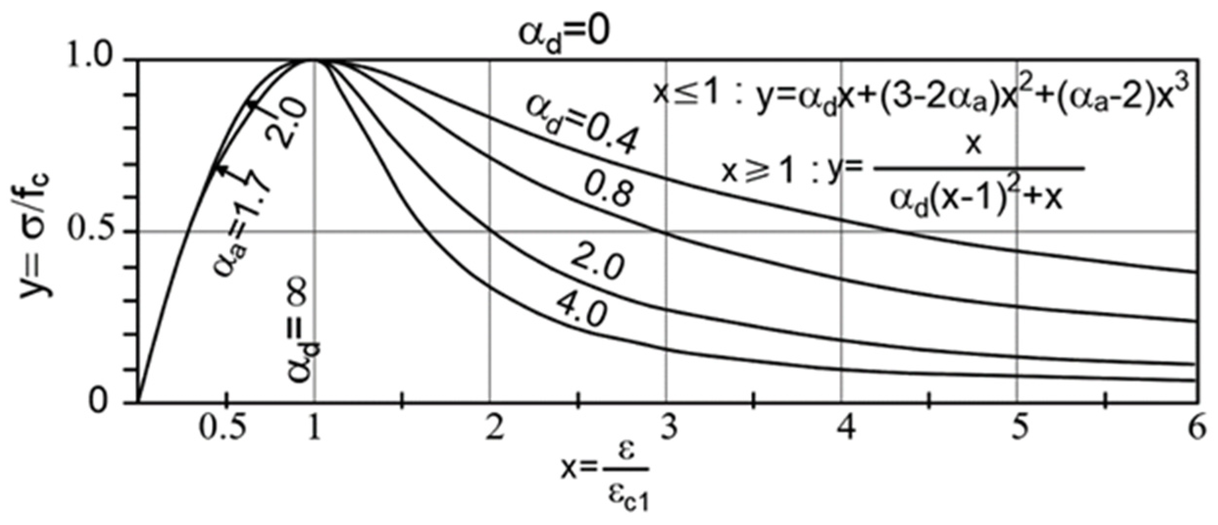
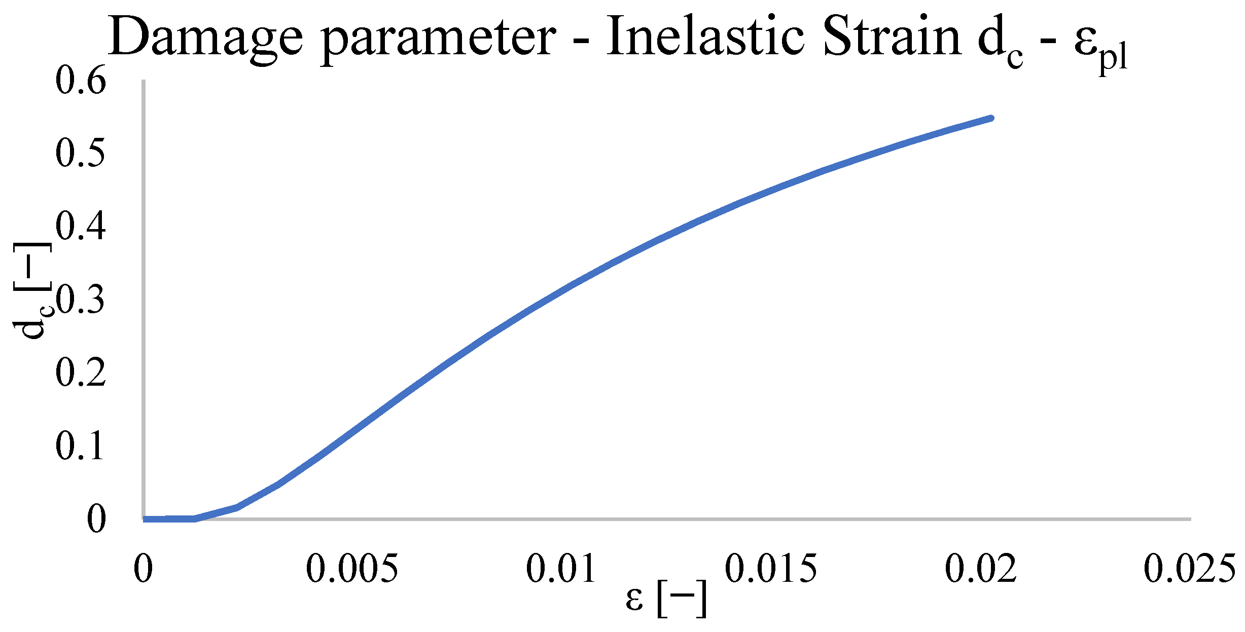
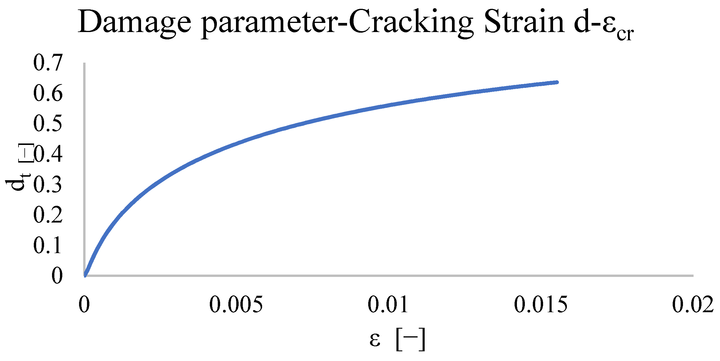
4.5. Concrete Damaged Plasticity: Calibration of the Mechanical Behaviour and Static Non-Linear Analysis Results

The Concrete Damaged Plasticity model is the most suitable for the analysis of wall panels, especially for the control of cracks, being a model in which the evolution of the failure domain and therefore of the parameters that govern its behaviour, is linked to the level of damage due to the plastic deformation ${\epsilon }_p$. Furthermore, the characterization of the model takes place through the implementation of uniaxial traction and compression $\sigma -\epsilon$ diagrams for which numerous publications on experimental tests are available in the literature, through which it is possible to carry out a direct control on the adherence of the results. analytics to real behaviour [13,14,15,16,17]. The uniaxial constitutive bonds were reconstructed according to the model proposed by Guo [18,19,20,21,22,23]. In the constitutive models of Concrete Damaged Plasticity, the elastic deformation ${\epsilon }_{el}$ and the plastic deformation ${\epsilon }_{pl}$, are calculated separately and then added together, to obtain the total deformation $\epsilon$. The elastic deformation depends on the elastic modulus and the Poisson’s modulus of the material, while the inelastic deformation is obtained through the stress-deformation curves. Below are the formulations for the construction of the behaviour curve of the material under a uniaxial compression regime, used for the definition of the reference curves for the calibration of the considered materials.

Elastic region:

$${\sigma }_c=E_{cm}·\epsilon$$

(112)

where $E_{cm}$ is the initial modulus of elasticity (stress of 0.3–0.8 $f_{bm}$) and $\epsilon$ is the generic deformation.

Inelastic region:

$${\sigma }_c=f_{bm} \left[{\alpha }_{a}x+\left(3-2{\alpha }_a\right)x^2+\left({\alpha }_a-2\right)x^3\right] x\le 1$$

(113)

$${\sigma }_c=f_{bm}·\frac{ x}{{\alpha }_d{\left(x-1\right)}^2+x} x>1$$

(114)

where:

$$x=\frac{\epsilon }{{\epsilon }_{c1}},{\alpha }_a=\frac{E_{cm}}{E_{c1}}, 0.4\le {\alpha }_d\le 4$$

(115)

$E_{c1}$ is the secant modulus corresponding to the maximum stress. The parameter ${\alpha }_d$ affects the shape of the descendant branch of the curve (Figure 21) and must be calibrated through experimental tests.

In Figure 22 and Figure 23, Stress—Inelastic Strain ($\sigma -{\epsilon }_{in})$ and Damage Parameter-Inelastic Strain ($d_c-{\epsilon }_{in})$ obtained by Equations (103), (104) and (108) are reported. The parameters adopted for the calibration of the compressive uniaxial behaviour [18,19,20,21,22,23] are reported in

Table 4. Parameters adopted for the characterization of the compressive uniaxial behaviour.

Ecm [MPa]	fbm [MPa]	εc1 [−]	Ec1 [MPa]	αa [−]	αd [−]	εyc [−]
1400	6.2	0.005	1240	1.29	0.4	0.0031

.

As regards the uniaxial tensile behaviour, also in this case an elastic region and an inelastic region are distinguished based on Guo [18,23]. The σ-ε constitutive law is described by the following relations:

Elastic region:

$${\sigma }_t=E_{cm}·\epsilon$$

(116)

where $E_{cm}$ is the initial tangent modulus of elasticity and $\epsilon$ is the generic deformation.

Inelastic region:

$${\sigma }_c=f_{btm}·\frac{ x}{{\alpha }_t{\left(x-1\right)}^{1.7}+x}$$

(117)

where ${\alpha }_t=0.312f_{btm}$ and $f_{btm}$ is the tensile strength of the material

$$x=\frac{f_{btm}}{E_{cm}}$$

(118)

In Figure 24 and Figure 25, the Stress-Cracking Strain ($\sigma -{\epsilon }_{in})$, and Damage Parameter-Cracking Strain ($d_c-{\epsilon }_{in})$ are reported, obtained by Equations (101), (102) and (107). The parameters adopted for the material characterization are reported in

Table 5. Parameters adopted for the characterization of the compressive uniaxial behavior.

Ecm [MPa]	fbtm [MPa]	εc1 [−]	αt [−]
1400	0.25	0.0001786	0.078

.

For the definition of the Flow Rule in Concrete Damaged Plasticity, it is necessary to provide the following parameters as input [22,23,24,25]:

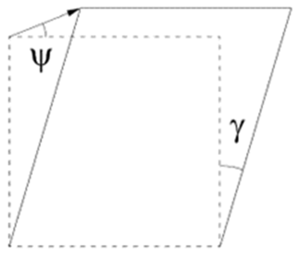
• 𝜓, dilation angle, in degrees [26];
• ε, flow potential eccentricity, is a small number with a positive sign, which defines the speed with which the hyperbolic flux potential approaches its asymptote, the recommended default value is equal to ε = 0.1;
• σ_b0/σ_c0, ratio between the initial equiaxial compression yield and the initial compression yield strength, the recommended default value is equal to s_b0/s_c0 = 1.16 and is the result of studies carried out by Lubliner and Lee [15,19];
• K, ratio between the radii of the meridians in tension and compression, the recommended default value is K = 2/3, the condition must be met according to which 0.5 ≤ K ≤ 1.0 in compliance with the convexity.
• μ–a viscosity parameter, it is considered only in the standard type Abaqus analyses and not in the explicit type analyses, for the visco-plastic regularization of the constitutive equations of the material, the default value is equal to 0.

The parameters used for the modelling in Abaqus of the Pavia Door Wall are reported in

Table 6. Parameters adopted for the characterization of Flow Rule.

𝛹 [°]	ε [−]	K [−]	σb0/σc0 [−]
20	0.1	0.5	1.16

.

In Figure 26 the comparison between the capacity curve obtained by CDP, DP, frame equivalent and experimental is reported. It is possible to notice how, in addition to the elastic branch and the perfectly plastic branch, in correspondence with the elbow of the experimental curve, the model obtained by the Abaqus software by implementing a Concrete Damaged Plasticity type bond with a damage function, has a trend extremely adherent to that of the curve experimental reference unlike the DP and equivalent frame models which differ, not following the branch of plastic hardening but going back up to a sudden transition to an almost perfectly plastic behavior. This result confirms the choice of the CDP model as a model to refer to for the modelling of wall panels, especially for the control of cracks, being a model in which the evolution of the failure domain and therefore of the parameters that govern its behaviour, they are related to the level of damage through plastic deformation. The insertion of a damage function is allowed only using a quasi-static explicit analysis which, however, is consistent with the large-deformation theory.

In Figure 27 the Von Mises equivalent stresses, for CDP model, are reported. The stresses, starting from a typical static distribution, as the horizontal action increases, are distributed along the main diagonals. The stresses are mainly focused on masonry piers and in the areas of nodal panels. Less stresses can be identified in the spandrel areas.

5. Conclusions

In this work macromechanical failure criteria and their application in the framework of the structural analysis are addressed, starting from the fundamental principles, passing through the theory of elasticity and plasticity, and arriving to the application of specific failure criteria in FEM simulations. Two of the more spread failure macromechanical models namely CDP and DP are used to model a benchmark case study called Pavia “door wall”. The FEM model developed in ABAQUS software is a solid, three-dimensional one with regular “Hex” meshes subjected to an appropriate partitioning procedure. The geometrically nonlinear analysis was performed using a quasistatic dynamic explicit in which the loads are applied smoothly. This type of analysis allows the use of damage parameters in compression and in tension combined with the Concrete Damaged Plasticity failure criterion. Paying attention to the results of the analyses conducted with the different failure criteria and methods of analysis, it is observed that:

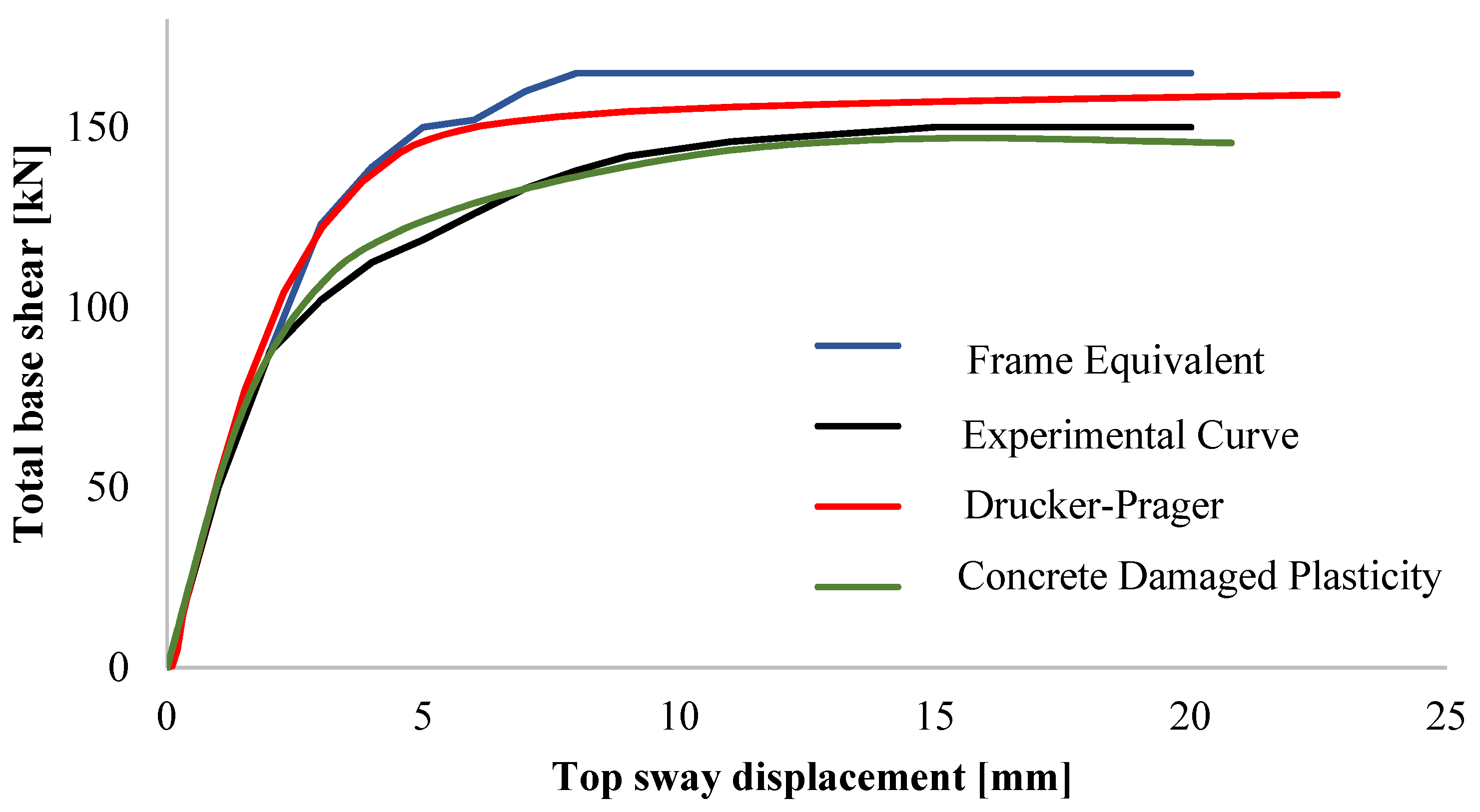
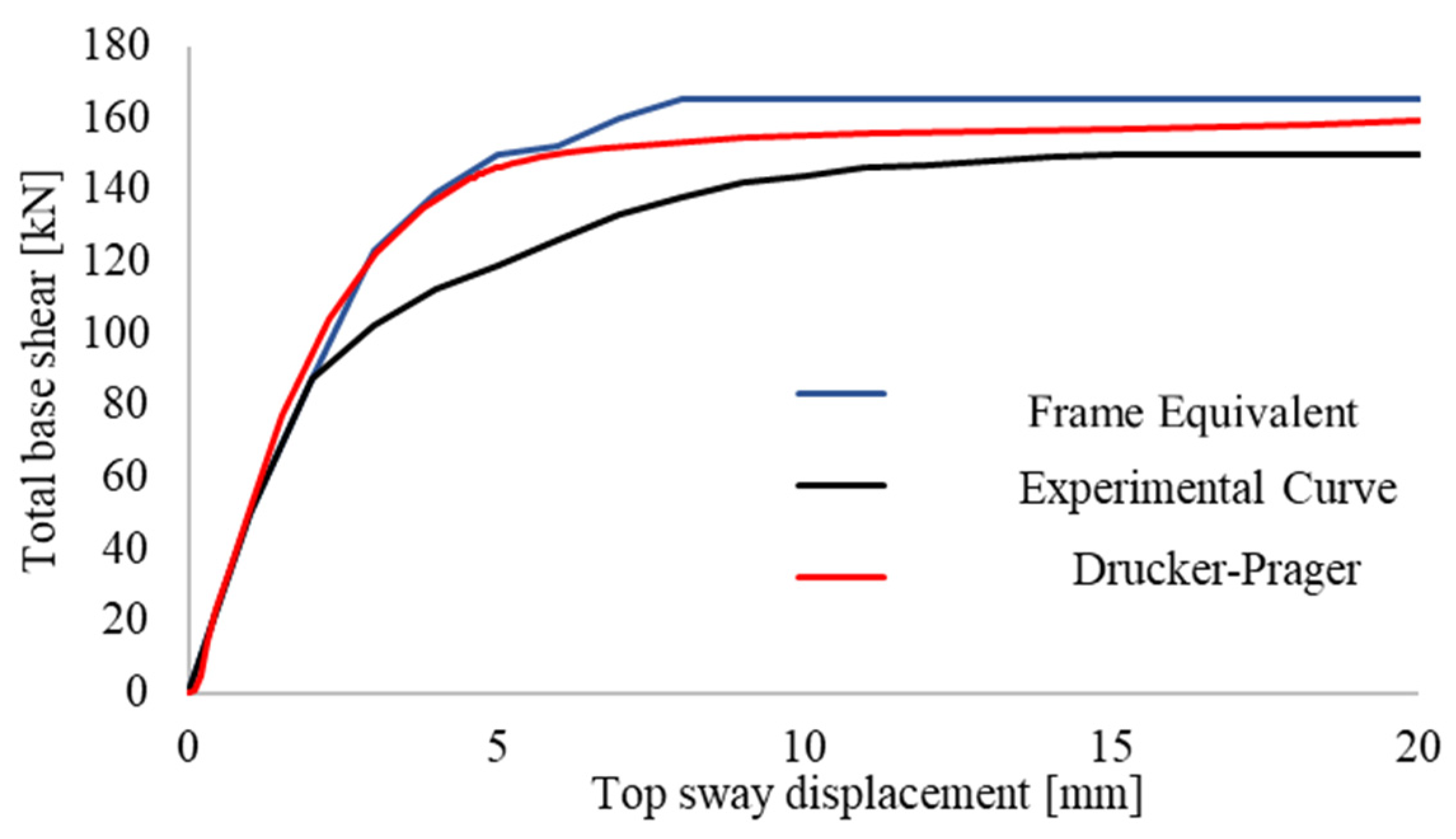
• all the curves fit well in the elastic range
• the only one that fits well in the knee zone of the pushover curve is the CDP Curve.

This result is probably linked to the possibility to catch the variation of the cohesion and the evolution of the damage given by Concrete damage Plasticity.

This result confirms that:

• the CDP model is suitable for the modelling of wall panels, especially for the control of cracks, because the evolution of the failure domain and therefore the parameters that govern its behaviour, are linked to the level of damage through the plastic deformation.
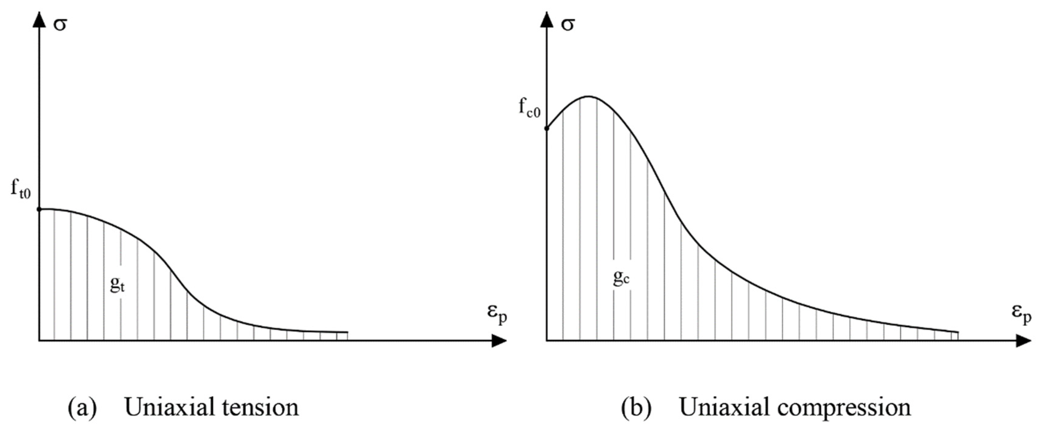
• The Guo model showed great flexibility and flexibility in the calibration process of uniaxial tension and compression curves.
• Sensitivity analysis demonstrated the importance of the calibration process showed in the paper for the definition of the uniaxial tension and compression curves.

The paper mainly aims at obtaining a high coherence between the experimental and analytical curves, in particular, when the masonry starts behaving in plastic range. This result was obtained only through the CDP criterion by means of an accurate calibration procedure of the uniaxial tension and compression curves, defined with the Guo’s model. The paper provides the tools to obtain a precise calibration, playing on the fundamental parameters characterizing the model. The importance of this result is justified by the need for high precision in defining uniaxial curves (as reported by the sensitivity analysis). The innovation, in this case, is derived from the combination of different existing theoretical bases to obtain an exact calibration model.

References

1. Guo, Z. Principles of Reinforced Concrete, 1st ed.; Butterworth-Heinemann: Oxford, UK, 2014. [Google Scholar]
2. Noor-E-Khuda, S. An explicit finite-element modeling method for masonry walls using continuum shell element. J. Archit. Eng. 2021, 27, 04021040. [Google Scholar] [CrossRef]
3. Sousa, R.; Guedes, J.; Sousa, H. Characterization of the uniaxial compression behaviour of unreinforced masonry—Sensitivity analysis based on a numerical and experimental approach. Arch. Civ. Mech. Eng. 2015, 15, 532–547. [Google Scholar] [CrossRef]
4. D’Amato, M.; Sulla, R. Investigations of masonry churches seismic performance with numerical models: Application to a case study. Arch. Civ. Mech. Eng. 2021, 21, 161. [Google Scholar] [CrossRef]
5. Calderón, S.; Sandoval, C.; Milani, G.; Arnau, O. Detailed micro-modeling of partially grouted reinforced masonry shear walls: Extended validation and parametric study. Arch. Civ. Mech. Eng. 2021, 21, 94. [Google Scholar] [CrossRef]
6. Shakor, P.; Gowripalan, N.; Rasouli, H. Experimental and numerical analysis of 3D printed cement mortar specimens using inkjet 3DP. Arch. Civ. Mech. Eng. 2021, 21, 58. [Google Scholar] [CrossRef]
7. Silva, R.; Costa, C.; Arêde, A. Numerical methodologies for the analysis of stone arch bridges with damage under railway loading. In Structures; Elsevier: Amsterdam, The Netherlands, 2022; Volume 39, pp. 573–592. [Google Scholar]
8. Al-Fakih, A.; Al-Osta, M.A. Finite Element Analysis of Rubberized Concrete Interlocking Masonry under Vertical Loading. Materials 2022, 15, 2858. [Google Scholar] [CrossRef] [PubMed]
9. Zizi, M.; Chisari, C.; Rouhi, J.; De Matteis, G. Comparative analysis on macroscale material models for the prediction of ma-sonry in-plane behavior. Bull. Earthq. Eng. 2022, 20, 963–996. [Google Scholar] [CrossRef]
10. Karaton, M.; Aksoy, H.S.; Sayın, E.; Calayır, Y. Nonlinear seismic performance of a 12th century historical masonry bridge under different earthquake levels. Eng. Fail. Anal. 2017, 79, 408–421. [Google Scholar] [CrossRef]
11. Nasiri, E.; Liu, Y. Development of a detailed 3D FE model for analysis of the in-plane behaviour of masonry infilled concrete frames. Eng. Struct. 2017, 143, 603–616. [Google Scholar] [CrossRef]
12. Abrams, P.D.P.; Calvi, G.M. Proceedings of the U.S.-Italian Workshop on Guidelines for Seismic Evaluation and Rehavilitation of Unreiforced Masonry Buildings; Technical Report NCEER-94-0021 20 July 1994; University of Pavia: Pavia, Italy, 1994. [Google Scholar]
13. Rizzano, G.R.; Sabatino, R.; Torello, G. Un nuovo modello a telaio equivalente per l’analisi statica non lineare di pareti in muratura. In Proceedings of the ANIDIS 2011 Italian National Conference on Earthquake Engineering, Bari, Italy, 18–22 September 2011. [Google Scholar]
14. Faella, C.; Consalvo, V.; Nigro, E. Influenza della snellezza geometrica e delle fasce di piano sulla valutazione della resistenza ultima di pareti murarie multipiano. In Proceedings of the Atti Dell’ VIII Convegno L’ingegneria Sismica in Italia, Taormina, Italy, 25–27 August 1997. [Google Scholar]
15. Chen, W.F.; Han, D.J. Plasticity for Structural Engineers; J. Ross Publishing, Inc.: Fort Lauderdale, FL, USA, 2007. [Google Scholar]
16. Kwon, Y.W. Revisiting Failure of Brittle Materials. J. Press. Vessel. Technol. 2021, 143, 4050989. [Google Scholar] [CrossRef]
17. Lubliner, J.; Oliver, J.; Oller, S.; Oñate, E. A plastic-damage model for concrete. Int. J. Solids Struct. 1989, 25, 299–326. [Google Scholar] [CrossRef]
18. Panoskaltsis, V.P.; Lubliner, J.; Monteiro, P.J. Rate dependent plasticity and damage for concrete. In Proceedings of the Engineering Foundation Conference, New Delhi, India, 5–10 January 1994; pp. 27–40. [Google Scholar]
19. Chen, W.F. Concrete Plasticity: Recent Developments. Appl. Mech. Rev. 1994, 47, S86–S90. [Google Scholar] [CrossRef]
20. Santos, C.F.; Alvarenga, R.C.; Ribeiro, J.C.; Castro, L.O.; Silva, R.M.; Santos, A.A.; Nalon, G.H. Numerical and experimental evaluation of masonry prisms by finite element method. Ibracon Struct. Mater. J. 2017, 10, 477–508. [Google Scholar] [CrossRef]
21. Lee, J.; Fenves, G.L. Numerical Implementation of Plastic Damage Model for Concrete under Cyclic Loading: Application to Concrete Dam; Rep. No. UCB/SEMM-94/03; Department of Civil Engineering, University of California: Berkeley, CA, USA, 1994. [Google Scholar]
22. Serpieri, R.; Alfano, G.; Sacco, E. A mixed-mode cohesive-zone model accounting for finite dilation and asperity degradation. Int. J. Solids Struct. 2015, 67–68, 102–115. [Google Scholar] [CrossRef]
23. Mousavian, E.; Casapulla, C.; Bagi, K. The Influence of Geometry on the Frictional Sliding of ∧ and ∨ Shaped Interlocking Joints in Masonry Assemblages. In Proceedings of the International Conference on Architecture, Materials and Construction, Lisbon, Portugal, 26–28 October 2022; pp. 37–45. [Google Scholar] [CrossRef]
24. Kujawa, M.; Lubowiecka, I.; Szymczak, C. Finite element modelling of a historic church structure in the context of a masonry damage analysis. Eng. Fail. Anal. 2019, 107, 104233. [Google Scholar] [CrossRef]
25. Calderoni, B.; Cordasco, E.A.; Guerriero, L.; Lenza, P.; Manfredi, G. Mechanical Behaviour of Post Medieval Tuff Masonry of the Naples area. Mason. J. 2009, 21, 85–96. [Google Scholar]
26. Grande, E.; Romano, A. Experimental investigation and numerical analysis of tuff-brick listed masonry panels. Mater. Struct. 2013, 46, 63–75. [Google Scholar] [CrossRef]
Figure 1. Haigh-Westergaard stress space.
Buildings 12 01245 g001
Figure 2. State of stress in the deviatoric plane.
Buildings 12 01245 g002
Figure 3. General shape of the meridian and the deviatoric sections for a pressure dependent material.
Buildings 12 01245 g003
Figure 4. Mohr-Coulomb failure criterion.
Buildings 12 01245 g004
Figure 5. Mohr-Coulomb failure surface and plane section.
Buildings 12 01245 g005
Figure 6. Mohr-Coulomb failure surface: meridian and deviatoric sections.
Buildings 12 01245 g006
Figure 7. Drucker-Prager failure surface and plane section.
Buildings 12 01245 g007
Figure 8. Drucker-Prager and Mohr-Coulomb matched surfaces in deviatoric plane.
Buildings 12 01245 g008
Figure 9. Extended Drucker-Prager matching in the deviatoric plane.
Buildings 12 01245 g009
Figure 10. Uniaxial stress-plastic strain curves in tension (a) and in compression (b).
Buildings 12 01245 g010
Figure 11. Concrete Damaged Plasticity model, TM, CM and deviatoric section.
Buildings 12 01245 g011
Figure 12. Vectors n _ , σ ˙ _ and n _ , ε p ˙ _ in stress (velocity of deformation) space, normality condition.
Buildings 12 01245 g012
Figure 13. Hardening rules: isotropic (a), Kinematic (b), mixed (c).
Buildings 12 01245 g013
Figure 14. Dilation angle in shear stress.
Buildings 12 01245 g014
Figure 15. Geometric scheme of the “Door Wall” in Pavia.
Buildings 12 01245 g015
Figure 16. Mesh pattern and partitions in ABAQUS, (a) Mesh pattern, (b) Mesh partitions.
Buildings 12 01245 g016
Figure 17. Concrete Damaged Plasticity in ABAQUS, uniaxial model for tension and compression.
Buildings 12 01245 g017
Figure 18. Concrete Damaged Plasticity in ABAQUS, load reversal from tension to compression.
Buildings 12 01245 g018
Figure 19. Concrete Damaged Plasticity in ABAQUS, evolution of the elastic modulus E in tension and in compression.
Buildings 12 01245 g019
Figure 20. Comparison among frame equivalent, experimental and Drucker-Prager pushover curves.
Buildings 12 01245 g020
Figure 21. Effect of the αd parameter on the descendant part of the curve.
Buildings 12 01245 g021
Figure 22. Uniaxial compression, stress-inelastic strain curve.
Buildings 12 01245 g022
Figure 23. Uniaxial compression, damage parameter-inelastic strain curve.
Buildings 12 01245 g023
Figure 24. Uniaxial tension, damage parameter-strain curve.
Buildings 12 01245 g024
Figure 25. Uniaxial tension, damage parameter-cracking strain curve.
Buildings 12 01245 g025
Figure 26. Comparison among frame equivalent, experimental, Drucker-Prager and Concrete Damaged Plasticity pushover curves.
Buildings 12 01245 g026
Figure 27. Von Mises equivalent stresses for CDP model.
Buildings 12 01245 g027